Article

Quality of Service Generalization using Parallel Turing Integration Paradigm to Support Machine Learning

1
Department of Cyber Security, International Information Technology University, Almaty 050000, Kazakhstan
2
Department of Computer Science and Engineering, University of Bridgeport, Bridgeport, CT 06604, USA
3
Department of Computer Engineering, International Information Technology University, Almaty 050000, Kazakhstan
4
Department of Management Information System (MIS), Gulf University for Science and Technology, Kuwait City 32093, Kuwait
5
Department of Computer Science, Joshi Research Center, University of Wright, Dayton, OH 45435, USA
6
Computers and Information Technology College, Taif University, Taif 21974, Saudi Arabia
7
School of Computer Science, Taylor’s University, Subang Jaya 47500, Malaysia
*
Authors to whom correspondence should be addressed.
Electronics 2023, 12(5), 1129; https://doi.org/10.3390/electronics12051129
Submission received: 13 January 2023 / Revised: 8 February 2023 / Accepted: 22 February 2023 / Published: 25 February 2023
(This article belongs to the Special Issue Application of Machine Learning in Big Data)

Abstract

:
The Quality-of-Service (QoS) provision in machine learning is affected by lesser accuracy, noise, random error, and weak generalization (ML). The Parallel Turing Integration Paradigm (PTIP) is introduced as a solution to lower accuracy and weak generalization. A logical table (LT) is part of the PTIP and is used to store datasets. The PTIP has elements that enhance classifier learning, enhance 3-D cube logic for security provision, and balance the engineering process of paradigms. The probability weightage function for adding and removing algorithms during the training phase is included in the PTIP. Additionally, it uses local and global error functions to limit overconfidence and underconfidence in learning processes. By utilizing the local gain (LG) and global gain (GG), the optimization of the model’s constituent parts is validated. By blending the sub-algorithms with a new dataset in a foretelling and realistic setting, the PTIP validation is further ensured. A mathematical modeling technique is used to ascertain the efficacy of the proposed PTIP. The results of the testing show that the proposed PTIP obtains lower relative accuracy of 38.76% with error bounds reflection. The lower relative accuracy with low GG is considered good. The PTIP also obtains 70.5% relative accuracy with high GG, which is considered an acceptable accuracy. Moreover, the PTIP gets better accuracy of 99.91% with a 100% fitness factor. Finally, the proposed PTIP is compared with cutting-edge, well-established models and algorithms based on different state-of-the-art parameters (e.g., relative accuracy, accuracy with fitness factor, fitness process, error reduction, and generalization measurement). The results confirm that the proposed PTIP demonstrates better results as compared to contending models and algorithms.

1. Introduction

The performance of machine learning depends significantly on the properties of the algorithms [1]. ML is made up of various cutting-edge algorithms that correctly predict events and help systems make informed judgments [2,3]. However, some of the current issues in ML include under-fitting, overfitting, bias, inconsistencies, and reduced accuracy [4]. Numerous algorithms have been developed, although they may not be entirely capable of solving these problems [5,6,7]. However, given the advent of digital and e-data, particularly in the fields of Big data and social networking data, ML has made appreciable development in data science [8,9].
Predictive analytics in ML uses a variety of models, approaches, and algorithms [10,11]. Recent research has focused on blending models and features [12,13,14]. To tackle bias, mistakes, overfitting/underfitting, and poor generalization, this work presents a novel technique of blending, in contrast to other recent advancements in data science research.
Many computations are performed concurrently to provide the solution more quickly. Therefore, faster computation and QoS provisioning can be made feasible by integrating the features of parallel computing and artificial intelligence (AI) [15]. Additionally, Turing can calculate complex tasks, which can be computed by any computer or supercomputer [16]. However, there is a need for the parallel Turing machine to increase the efficiency of given models and algorithms. Thus, the model is trained using the suggested PTIP paradigm to determine the supporting algorithm, and it is then blended to increase the prediction accuracy and classifier fitness. The concept, questions, contributions, and anatomy of the article are introduced in the next subsections. Our motivation stems from the fact that we are using data from social networking in conjunction with academic and professional data to enhance predictive analytics. Several cutting-edge algorithms have been studied [17,18] to comprehend the proposed PTIP paradigm. The following general research questions are what this work aims to explore and answer:
Can matching, fitness, and accuracy ratings be used to fine-tune and combine algorithms?
Is it possible for a blended model to perform better than a single algorithmic model when it comes to handling bias, over- or under-fitting, poor generalization, and low accuracy?
Can error be used/programmed to govern the model for lower and upper bounds to avoid bias and over-learning?
Can algorithms be added and deleted algorithmically in real-time as the classifier processes the provided raw data for ML predictions?
Can overfitting and underfitting be pushed to a logical space of the optimum fitting?
Finally, can a blended model learn from its incorrect predictions?

1.1. Research Problem

The main challenge that data scientists, researchers, and analysts come across is to know which algorithm or model is the best for the problem(s)/data to be used? There are many unknowns and uncertainties. Each algorithm may behave differently for different dataset and variables/features. Evaluation of a model or algorithm is crucial for various classifiers. It becomes highly challenging to choose a classifier type based on new or unseen data. The standard rule adapted by the scientists and researchers is assessing some of the classifiers that algorithm produces [19]. We consider this as a research problem to see if an improved model with algorithms, uniquely engineered with built-in parallel processing, can be introduced for such predictive modeling using enhanced blending and tuning.

1.2. Research Contributions

We see the potential of data science in the creation of new algorithms as well as enhancements to current strategies, while considering the most recent requirements and applications in the big data environment. The following is a summary of the paper’s contributions:
The proposed PTIP has the ability to measure the accuracy, fitness, and matching scores in order to create a blended process;
The proposed approach demonstrates that blending is performed depending on how well each algorithm, as chosen from the pool of options, fits the sort of data model being trained. Furthermore, the proposed approach guarantees that the model is neither biased nor overfit in comparison to any particular algorithm;
The proposed classifier is trained to be able to add a good-fit algorithm (one with better metrics) or get rid of a bad-fit algorithm (one with inferior metrics);
The enhanced metrics, which control the model’s performance dimension, are produced. In this manner, the proposed approach is simultaneously cross-checked while learning from the data (during training);
The proposed model’s design is represented in 3-D logical space. In addition, the proposed model is shifted to z-space coordinates to get the optimal fitness;
A novel strategy to using a meaningful measure in machine learning is created (i.e., Error). The presented model has been trained to be managed by minimum and maximum error-bounds. As a result, acceptable bias and fitness, including overlearning, may be preserved. The lowest and maximum error boundaries for GG and LG are 20% and 80%, respectively.

1.3. Paper Structure

The remainder of the paper is structured into the following sections:
Section 2 presents the salient features of the current studies. Section 3 outlines the proposed parallel turning integration paradigm. Section 4 presents the experimental findings and discussion. In Section 5, the entire article is concluded.

2. Related Work

This section summarizes the most important aspects of existing approaches. Ref. [20] described an iterative approach for continuous variational methods that use the boundary value issues. More specifically, they investigated a parallelization technique that makes use of the capability of multiple cores GPUs (graphics cards) and CPU (Central processing unit). They also investigated the parallel technique for first- and second-order Lagrangians and demonstrated its superior performance in two intriguing applications: a fuel-optimal navigation issue, known as Zermelo’s navigation problem, and an extrapolation problem. The cross-modal Turing test was used as an all-purpose communication interface that enabled an embodied cognitive agent’s “message” and “medium” to be tested against another [21]. Two competing modules might undergo a sequential cross-modal Turing test with the usage of reciprocating environments and systems. Such a strategy could prove to be crucial in systems that require rapid learning and model adjustment, (e.g., cyber-physical systems), which are formed at the intersection of many technical–scientific engineering solutions. This strategy may be successful in the field of transfer learning, where a pre-trained network fragment might well be linked with input that is essentially unrelated to neural networks.
Researchers looked into potential increases in sampling efficiency [22]. To depict computationally ubiquitous models, a polynomial-time Turing machine was utilized, and Boolean circuits were used to represent artificial neural networks (ANNs) functioning on finite-precision digits. Direct connections between their inquiry and the outcomes of computational complexity were shown by their study. On the anticipated increases in sample efficiency, they offered lower and upper bounds. The input bit size of the required Boolean function defined their bounds. They also emphasized the close connections between the intensity of these limitations and the standard open Circuit Complexity concerns. Deep learning in machine learning seeks a general-purpose computing device that could carry out challenging algorithms resembling those in the human brain. Neural Turing Machine (NTM) integrated a Turing machine with a long-term memory, which was used as a controller to accomplish deep learning techniques [23]. Basic controllers are used by NTM to carry out a variety of simple and sophisticated tasks, including sort, copy, N-gram, etc. Complex jobs, such as classifications, were disregarded, and NTM’s weights could not be improved.
Super-Turing models’ expressiveness hierarchy was introduced [24]. A-decidable and i-decidable algorithms (e.g., D-complete, U-complete, and H-complete) complexity classes—inspired by NP-complete and PSPACE-complete classes for intractable problems—were introduced as first steps. Similar to how to approximate, randomized and parallel algorithms enabled workable solutions for intractable problems. This study might be seen as the first step toward feasible approximations of answers to the Turing machine’s inherently unknowable issues. All of the existing methods focused on decision making and model adjustment. Contrary, the proposed PTIP is able to quantify the matching, fitness, and accuracy scores to establish a tuning and blended process. The proposed PTIP also ensures that the model is neither overfit nor biased, as compared to any single algorithm under test. Furthermore, a distinctive approach of employing a significant metric in machine learning (i.e., Error) is developed. Finally, the proposed model is trained to be administered by minimum and maximum error bounds. Thus, acceptable bias and fitness including overlearning can be maintained. The contemporary nature of existing approaches is given in Table 1.

3. Proposed Parallel Turing Integration Paradigm

The latest trend in the ML research [25] has shown an immense potential to evaluate various algorithms in parallel [26]. We take a research opportunity to enhance the accuracy for the state-of-the-art algorithms of the ML. The proposed PTIP consists of four components to play an important role for accuracy enhancement of the ML algorithms.
Improved Machine Learning Engine
Develovement of Pre-processing Internals
Measurement and Risk Optimization
Final framework of PTIP

3.1. Improved Machine Learning Engine

The proposed PTIP leverages the features of an improved machine learning engine (IMLE) that increases accuracy depicted in Figure 1. The IMLE consists of state-of-the-art components, which help guarantee the QoS provision, especially accuracy. The PTIP is discussed at the abstract level.
Enhanced Algorithms Blend and Turing (EABT): The EABT uses ensemble, bagging, and boosting to choose the best blend until the improved metrics are evaluated, then it applies the current ML and predictive modelling techniques (e.g., Logistic Regression, Linear Regression, Multiple Regression, Bayesian, Decision trees, SVM, and Classification). This scheme exploits the potential of parallel processing of the techniques. Errors and bad predictions made during a test are sent back to the algorithm in this phase so it can continue to learn from its errors (AI).
Enhanced Feature Engineering and Selection (EFES): It improves feature engineering to extract more information (e.g., feature development and transformation). Finding the best collection of characteristics or features for the relationship between “predictor-target” variables is the best fit. Additionally, it makes sure to include features with the greatest fitness scores and eliminate features with the lowest. Each feature may be validated by the EFES.
Enhanced Weighted Performance Score (EWPM): It ensures that the model should neither be overfit nor underfit by generating a unique metric based on standard metrics. It also acts as the measuring instrument to ensure the precision of overall performance metrics.
Improved Cross Confirmation and Split (ICCS): This component develops and employs a novel strategy to train-test data splitting in order to improve existing validation approaches such as cross-validation.

3.2. Development of Pre-Processing Internals

The pre-processing internals reduce the inaccuracies in the datasets. Therefore, the pre-processing internals can be created using the Logical Table (LT). The complete modular details of the Logical Table (LT) are outside the scope of this article. However, the brief detail is provided. The method that best fits the PTIP is to use of the logical table, which expands with the quantized output. We determine that the proposed model’s minimum value is where LT controls the process. According to Algorithm 1, it makes an entry for each dimension (X, Y, and Z). The threshold value is set for the LT; if the LT value < 0.5, binary “0” is assigned; if ≥ 0.5, binary “1” is assigned. Thus, the binary truth table can be formed from those values. The primary goal of Algorithm 1 is to employ LT to produce pre-processing internals in order to correct the inaccuracies in datasets.
Steps 1–2 of Algorithm 1 depict the input and output procedures. The variables utilized in the Algorithm 1 are initialized in steps 3–5. The logical table objects and nodes are created in step 6. The IMLE is generated in step 7 to increase accuracy. Step 8 configures the IMLE’s component (FFES) (which helps to increase accuracy). The value for error removal in the IMLE is shown in steps 9 through 12, and the error removal procedure continues until no more errors are found, in every direction. Step 13 involves the error and data validation processes.
Step 14 provides the distance function’s correct arguments. Steps 15–16 show the activation processes of Turing and blended functions, which provide the alert on the logical table. If an error is discovered, the error classifier functions of B A ,   T A are invoked and the best set of features is determined in steps 17 through 19. The alert is set on the logical table to identify errors in tuples and blocks in step 20. Additionally, steps 21–22 establish the ideal fitness range. The suggested PTIP has an updated logical table. Step 23 involves setting the strategy function for each dimension. The classifier sets and triggers the cost function for error and data validation. If a value of error < 0.5 is found inaccuracy removal is commenced, and the logical table is eventually modified in steps 24–30.
Algorithm 1: Inaccuracy removal ψ n in logical table for development of pre-processing internals
  • Input: A . P = A 1 ,   A 2 ,   A 3 , .. ,   A n , Raw Dataset DS sig , noi
  • Output: ψ n
  • Initialization(A): {   S x . y , z : strategy function for all dimensions;   Op . F : optimal fitness; C : cost function}
  • Initialization(B): IMLE ,   EFES
  • Initialization(C): { A : error,   A n : total number of errors;   H i p i : entire datasets;   H i p i : removal of data; d A 1 ,   A 2 : distance between two data items; D ,   t : arguments of distance function; B A : blended function for algorithm; T A : Turing function; LT : alert on logical table;
  • Generate LT object, Nodes
  • Generate IMLE
  • Set FFES ,   EWPM ,   ICCS , EAB
  • While ( ψ n ) 0.5     e , E   IMLE Do
  • Create Logical Table Object LT x , y , z
  • For each (A A n ) Do
  • Compute d A 1 ,   A 2 = i = 1 M H i p i H i p i 2  
  • Validate (A A n ) and d A 1 ,   A 2
  • Compute D ,   t  
  • Compute LT.   B A ,   T A
  • If LT B A ,   T A then
  • Retrain classifier ( B A ,   T A )
  • Update EFES D ,   t
  • End If
  • Compute Op . F 0 : 1
  • End For
  • Update: LT of PTIP
  • Set S x . y , z = j = 1 N ( D j ,   τ ( p j ,   S x , y , z )
  • Set C
  • If (C is flagged by Classifier) then
  • Compute d A 1 ,   A 2
  • Detect ψ n
  • Update LT
  • End If
  • End While
LT operates in the memory and is dynamically updated. It keeps track of the algorithms A x , y , z = { A 1 , A 2 , ......... ,   A n , } as the ML process evolves to accomplish the final optimum fitting after it has incorporated all the algorithms from the pool. This helps achieve the optimum blending and tuning. This logical table stores data based on three dimensions, where ‘x’ = overfitness, ‘y’ = underfitness and ‘z’ = optimum-fitness.

3.3. Measurement and Risk Optimization

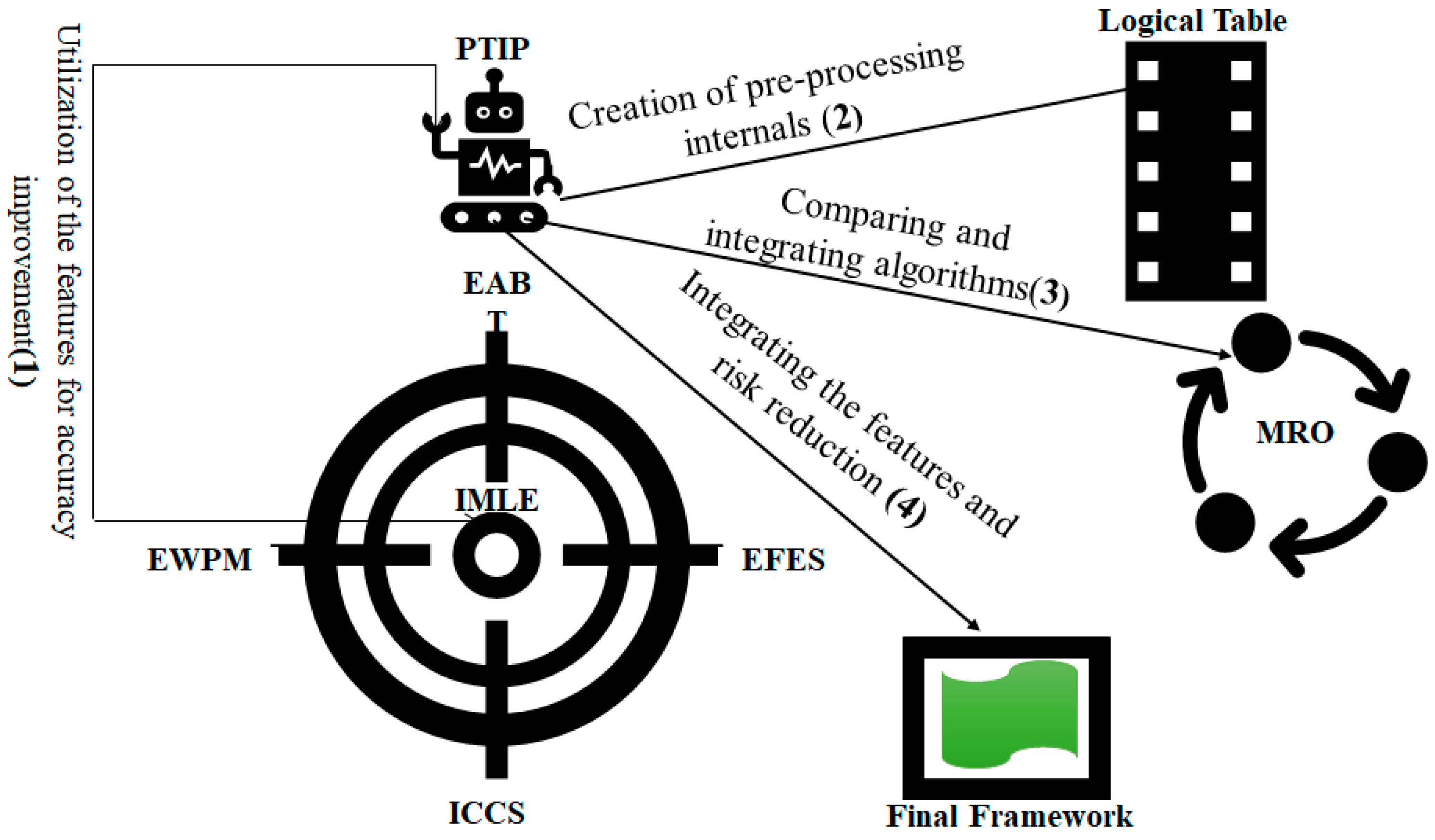
The measurement and risk optimization (MRO) component deals with applying various algorithms one by one to observe the outcomes (i.e., measures), and then prepares the model for risk estimation and algorithm blending. This construct also compares the two algorithms at the same time and then groups them based on Euclidean distance for similarity scores in terms of fitness. This sub-model finally produces the set of algorithms for the best fit for a given dataset. The end goal is to engineer inaccuracy removal that can be done through classifier function.
Let us define that standard distance function, which consists of d A 1 ,   A 2 that demonstrate the distance between two data items. The H i p i can be identified as entire datasets, and H i p i be the removal of data from the datasets.
d A 1 ,   A 2 = i = 1 M H i p i H i p i 2
Let S be the strategy function for all dimensions, and p i is the training problem set (dataset vector) in distribution of time D ,   t being the arguments for distance function in .
S x . y , z = j = 1 N ( D j ,   τ ( p j ,   S x , y , z )  
Therefore, the correct arguments of distance function can be calculated as:
D ,   t = T ¯ D + 1                                                                                                 t =   t D + 1                                                               e   N ,         T ¯   T
Theorem 1. 
Algorithm evaluation process A 1 ,   n makes suitability scores for the fitness.
Proof. 
Let d A 1 ,   A 2 be the Euclidean distance between the two algorithms since there must be a matching factor (M.F) for the best fitness between them. Thus, O p . F 0 : 1     0.5 , as optimum Fitness scores and 0.2 e r r E r r 0 : 1 < 0.8 , are bounds of LE (err) in GE (Err).
With the pointers x denoting Overfitness, y denoting underfitness, and z denoting optimal fitness, let S x . y , z compute the appropriateness scores for the fitness of the provided method in 3-D space. Let ψ n be the classifier function, which the model learns to categorize in order to be able to identify the ideal combination of methods for a particular dataset and issue. □

3-D Cube Logic for Security Provision

In encryption transmission, the 3D cube logic is used to maintain a security, and the activity is carried out based on the pattern generated by the transmitting side rather than supplying the whole cube structure. A key that is utilized for encryption and decryption is deduced through a sequence of steps that match the 3D CUBE pattern.
The proposed technique decrypts the encrypted text provided by the receiver using a key derived by completing the shuffling of 3D CUBE based on artificial intelligence (AI), which overcomes the challenge of secured key exchange by removing the key exchange procedure from the conventional symmetric key encryption. Because it is impossible to deduce a key used by a third party using AI-based learning, the 3D CUBE logic can also provide higher security than the conventional symmetric key encryption scheme.
As it is used to handle keys and transmit them correctly in the symmetric key encryption system, the procedure after generating the key in the 3D CUBE technique is identical to that in that mechanism. In the symmetric encryption system, instead of participants sharing keys used during initial encryption communication, the transmitter sends a 3D element key pattern as a randomized 3D CUBE sequence by which the key can be activated, and the recipient obtains the secret key by incorporating it through AI-based learning. By using the XOR operation on the sequence’s 3D CUBE pattern, the secret key is formed here based on the randomized order as a sequence.
Assume a dataset D e s sig , noi , where “sig” denotes the signal and “noi” denotes the noisy component of the dataset that can be transmitted. The classifier function with a loss function L x , y , z |   0 : 1 , for which we loop in n-sample blocks such that loss function remains in the defined boundary as estimated, for which the feature sets exist in the function F = { f 1 ,   f 2 ,   f 3 , .. , f n with optimal score > 0.5. The classifier for the upper boundaries of generalization error in the probability Ć x , y , z , for n blocks of data sample can be provided by:
Ć x , y , z = L x L y L z + 1 n   k = 1 n U . D e s L . D e s k + log p 2 2 φ 3
where φ is the pattern identified as signals (removing noises) with the probability of 1 − p. Here, we create a straightforward approach to calculate the loss function in noisy and signal data(N) that affects classifier construction.
L ( D S ( S x , y , z , N x , y , z = 0 ,     N ( x , y , z 0.5   S x , y , z )   1 ,     S x , y , z 0.5   N x , y , z
Thus, for each algorithm in the pool, the optimum fitness can simply be determined as:
O p . F 0 : 1 =   ( Ć x , y , z L ( D S ( S x , y , z , N x , y , z   2 × log e r r 2 e r r + E r r
Based on the Equations (4)–(6), the optimum fitness values can be calculated, which are given in Table 2.
As previously mentioned, our model is built on 3-D space for the x, y, and z dimensions, which the algorithm employs to optimize the blend’s fitness (Op.F) to the supplied data. It is important to highlight that using this technique, the model is designed to be highly generalizable for any supplied data with any kind of attributes. We thus engineer the mix utilizing matrix (real-valued) space manipulation and the Frobenius norm provided by:
M x , y , z = x = 1 X y = 1 Y z = 1 Z M x , y , z 2
The matrix manipulation for each dimension to evaluate the blend can be built as:
ψ n = E x t r a c t x , y , z   Z ( M x , y , z ) + log k = 1 Z γ z + 1   .   O p . F 0 : 1
The illustration in Figure 2 supports the mechanics of the Theorem 1. As we observe the visualization of three functions, err|Err ( e / E ) , Op.F and Cost (C) being rotated based on distance function, as shown. Thus, Blender Filter Switch (logical) connect the value to the Suitability and Evaluation Score 3-D logical construct. The value of ψ n in each dimension swing between 0 and 1, based on Op.F response from Tuning Synthesizer block. Table 3 shows the results of developed functions.
Theorem 2. 
Risk Estimation, Local Errors, and Metrics Evaluation A l g o . R i s k e m p f
The algorithm generalization evaluation error {AGE(Err)} is inbound of all LE err(n), for which each occurrence of the error at any point in x and y space, exists inside all theoretical values of Err, such that e r r A E r r A + 1 ,   w h e r e   0.8 < e < 0.2 . Let there be a maximum risk function (Φ) with mean square error M S E on the set of features as F = f 1 ,   f 2 ,   f 3 ,   ...... ,   f n , and unknown means as m 1 ,   m 2 ,   m 3 ,   ...... ,   m n .
The algorithm generalization assessment error, or AGE(Err), is an aggregate of all LE err(n), in which each instance of the error at any location in x and y space occurs within all conceivable values of Err, so that e r r A E r r A + 1 ,   w h e r e   0.2 < e < 0.8 . Assume that the maximum risk function (Φ) has unknown means (m 1, m 2, m 3, m n) and mean square error (MSE) on the set of features (F= f 1, f 2, f 3, …, f n).
Construction. 
To prevent underfitting and overfitting in terms of the errors to be regulated by the upper and lower bounds. We construct the minimum and maximum error boundaries logical limit. We initially force the mistake to be at a low threshold before making it high. The algorithm then learns to keep between the min(e:0.2) and max(e:0.8) boundaries, and accuracy is obtained.
m a x e : 0.8 = 1 E   i = 1 N e { ( R M S E i ) 100 + 0.2 / E }
m i n e : 0.2 = 1 E   i = 1 N e { ( R M S E i ) 100 + 0.8 / E }
Let us define our optimum error (dynamically governed by algorithm tuning and blending process), as:
E o p t   ( m a x ,   m i n   | e x , y , z = x , y , z 1 E × j = 1 N t max e j min e j   *   g . f
where the PTIP algorithm generates (g.f), the error gain factor. Each method tends to cause more mistakes when they are combined, hence the combined errors of both global and local functions must stay within the given range. There are two types of errors for generic machine learning modelling: estimation and approximation [27]. Its collective name is generalization error, and finding a specific function f′(x, y) that tends to reduce the risk of training in the targeted space is what we aim to do in this case (i.e., X, Y, Z), shown as:
R i s k f x , y , z = X × Y × Z L   y ,       f x , y   P x , y , z d x d y d z
Figure 3 shows the concept of correlation of error bounds and risk function. As we propose the novel idea of limiting the error between 20% and 80% for optimum realistic fitness for the real-world prediction, it shows that the Risk Estimation (emp) stays in bounds of logical cube shown on the right. The center point shows the ideal co-variance of function ն . P (x, Y, Z) will be unknowable at this time. Based on the “empirical risk minimization principle”, which is statistical learning theory that can employed to determine the risk.
R i s k e m p f = 1 m   i = 1 m L   (   y i   ,   f   x i )
Here, we require to fulfill two conditions, which are given below:
(i)
lim m   R i s k e m p f = R i s k f x , y , z
(ii)
l i m m     min f     H R i s k e m p f = m i n f     H   R i s k f x , y , z .
These two conditions could be binding when H is comparatively trivial. The second condition needs minimal convergence. Thus, following bound can be constructed that is being held valid with probability of 1 − δ is R f     R i s k e m p f + ɀ   . Thus, ɀ can be determined as:
ɀ = h   ln 2 m h + 1 ln δ 4 m  
The sub-estimator function is m k ^ = c F k , ϑ . Hence, the regularization parameter ϑ is positive and it has been observed that the sub-estimator function c F k , ϑ = F such that, ϑ = 0   |   m i ^ = F k . We deduce that ϑ = , corresponds to maximal shrinking, which is m k ^ = 0 ,   f o r   k = 1 , , , , , , n . In this case we use Stein’s unbiased risk estimate (SURE) and cross validation (CV) technique, where prominent estimators include (lasso), (ridge) and (pretest). We use the squared error loss function, sometimes called compound loss, as the basis for loss and risk estimation.
L o s s n F ,   c k , ϑ ,   D = 1 n   k = 1 n c F k ,   ϑ   m k 2
where D = d 1 , d 2 , , d n shows the distribution of Features F {p, q, r}. It should be observed that Loss is highly dependent on ‘D’ through value of ‘m’. We can construct the regularization parameter for which the algorithm blend fits the model to maximum relevance, such that: ϑ D = max ϑ   0 , B   c .   ,   ϑ ,   π .
Therefore, the risk of algorithm A l g o . R i s k e m p f can be calculated as:
A l g o . R i s k e m p f = R i s k f x , y , z × E D G E L o s s n ɀ n
Consequently, Equations (15) and (16) can be used to determine the maximum risk of algorithm Φ .
Φ = max A l g o . R i s k e m p f + lim 0.2 < e r r < 0.8 R i s k f x , y , z  
where R i s k f x , y , z is the risk of distribution features of algorithm.
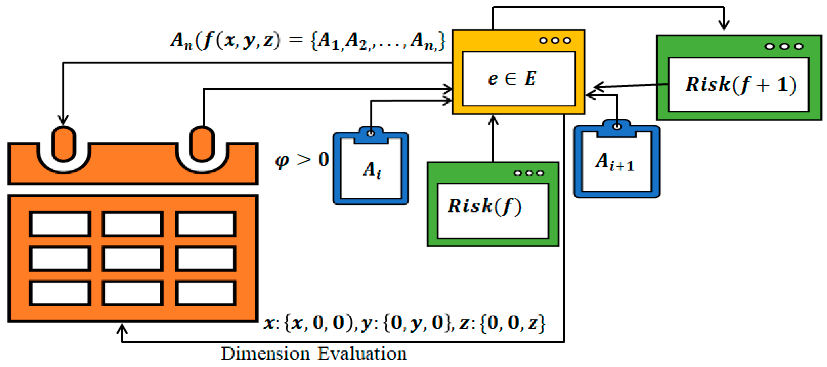
The risk estimation process of algorithm in 3-d space is depicted in Figure 4 to support in-bound local evaluation (LE) and global evaluation (GE).
Algorithm 2 maximizes fitness, this algorithm computes the risk estimation function, local error bounds, and metrics evaluation. It builds on Theorem 1. It tunes the blend to stay within error bounds for ensuring optimum fitness based on the Risk Estimation Function and observed errors, and then assesses metrics to ensure the blend’s overall performance.
Algorithm 2: Computation of risk estimation process
Input: ψ n : classifier Function, F n : Features set for sampling
Output: Φ ,   Risk emp f ,   e ,   E , Ё
Initialization: e     0 ,   E     0
  • Create: LTObject, NODES i N , PTIP
  • Generate ObjectIMLE(h)/* Generate an object reference for improved machine learning engine application programming interface (API)*/
  • Set ObjectIMLE.PublicFunctions(h.IMLE, h.EFES, h.EWPM, h.ICCS)/* managing the four constructs*/
  • While ( e 0.2   OR 0.8 ) Do
  • Compute max(e) and min(e) bounds
  • Compute j   = 1 Nt max e j min e j   *   g . f /* The optimum error function */
  • Create Logical Table Object LT x , y , z
  • Create h.ICCS( S 1 , S 2 , , , , , , S n )   /* Create Test Train Split using ICCS library. */
  • For (Each node in NODES i N ) Do
  • Compute Risk emp   f     1 m   i = 1 m L   ( y i ,   f   x i
  • Compute Loss Function 1 n   k = 1 n c F k ,   ϑ   m k 2
  • If ( ϑ D     Last   updated   max ϑ   0 , B   c .   , ϑ ,   π ) then
  • Replace ϑ D
  • Recompute Loss Function
  • End If
  • Compute ɀ
  • Set R f     Risk emp f + ɀ
  • Examine error bounds for regularization
  • If (error > 0.2 and < 0.8) Then
  • Update the LTobject.LT(x, y, z)
  • Update x, y, z from Logical Table
  • End If
  • End For
  • Compute ( Algo . Risk emp f , LT)
  • Compute Φ
  • Compute e, E and E opt /*Using Risk Function and LTobject Update *
  • End While
  • Return Φ ,   Risk emp f ,   e ,   E , E opt
Theorem 3. 
A l g o . B l e n d p , q , r , A l g o . G G ( p , q , r ,   and A l g o . E r r o r p , q , r support the parallel Turing integration paradigm.
Proof. 
Let us take the pools of the supervised learning algorithms such as A p , q , r = A 1 , A 2 , ......... , A n   , which acquires the given data D s = ds 1 ,   ds 1 ,   ds 3 , ........ , ds n ; thus, the correlation exists. Therefore, matching factor M f can be expressed as M f p 0 , q 0 , r . The LG exists for each algorithm such that GG is available in optimized fashion that is illustrated as g     1   | | ( A     { 1 , 2 , .   .   .   , n ) . The optimization functions exist for each algorithm. Therefore, each algorithm possesses the set of predictor characteristics, such that S input = 1 , 2 ,   .   .   .   , T n , and targeted variables, S output = 1 , 2 , 3 , 4 ,   .   .   . ,   T n . Thus, each given algorithm A performs well in the blend for each set of features S f e . Hence, the enhanced weighted performance metric W p m should be   0.75 for each specified parameter, which remains above the threshold value of the measurement until W p m falls below 0.75. Therefore, A   All   in   A x , y , z 0.1 . The LE becomes very unstable in blend, and thus the model creates a complex error function ( E x , y , z , such that e   E   |   log E e 1 > 0, and let be the measure of complexity of the GE within a probability p   > 1   δ   ,   where   all   δ     1 p p 2 . There must be a hypothesis “h” on GE that travels in the x, y, and z directions. It shows nonlinearity that is dependent on the number of algorithms in the blend. Moreover, it is distributed linearly throughout the space in the LE. □
Construction. 
The E d , H d , M d functions can be employed in the space. The optimum GG is used for induction. Therefore, Euclidean distance can be used for measuring the distance that is given by:
E d = x 1 x 2 2 + y 1 y 2 2
Similarity can then be obtained using Hamming distance H d , which is specified by:
H d = j = 1 k x j y j
Thus, Minkowski distance M d can be calculated as:
M d = j = 1 k x j y j p 1 p
We create the related matching factor (MF) based on these data at the point when each distance reduces to the smallest potential value with the least amount of theoretical GE (Err).
M F x , y , z = 1 S i = 1 n A i ± E d + H d + M d n ,   E r r < 0.5
The triangles are built for our blend using the 3-D space and axis align method. Let Δ = Δ 1 , Δ 2 ,   Δ 3 , .......... , Δ n , which specifies the immeasurable number of triangles in disseminated fashion which are given as:
Δ x , y , z a , b = W ( x a   ,   y b ,   z   a b   :   a   b ,   a n d   a b > 0
The following function describes the search for optimal coordinates: where W = 1 ,   a   b 0 ,   a b > 0 and EWPM is obtainable through IMLE API. Let us assume that EWPM should remain above 0.5 for optimal zone in the 3D rational space. Thus, the co-ordinates for the y-axis can be expressed as:
Y i = α + α β 1 β n 1 X i , 1 + ........   α β 1 β n n X i , n + ϵ i ,   Where   ϵ = ϵ 1 ϵ 2 ... ... ϵ n   in   each   dimension
As a result, given corresponding values and blend of the algorithms switches from multidimensional space to lower dimension. After tuning has been accomplished (Theorems 1–3), an error happened as a complicated function, dependent on a variety of variables and the fundamental blend of algorithms. The global err is displayed in Figure 5 as every algorithm’s LE is no longer applicable mathematically. The Each algorithm’s standard deviation error ( σ ) tends to rise when it is coupled with another algorithm. A common statistical method that models relationships between n+ variables using a linear equation to determine its fitness is developed by:
S t a n d a r d   D e v i a t i o n   E r r o r = σ = j γ 2 j   n p 1
y i = f x = 0 ,     I f   e r r o r   f a l l s   a b o v e   t h e   t h r e s h o l d 1 ,     I f   e r r o r   i s   a c c e p t a b l e .
The distribution can be written using Bernoulli Distribution process:
Y i :   P r o b Y i = y i   = π i y i 1 π i 1 y i  
The bounds of 20% and 80% should be tuned. The small circles demonstrate the x , y , z infinite space in the logical cube depicted in Figure 6. Note that each point varies between 0 and 100%. It is ideally used when output is binary, such as 1 or 0, Yes or No, etc. A logit function governs the linear model in LR. Thus, we can finally construct using Equation (25).
E r r 2 = E r r M e a s u r e d E r r C a l c u l a t e d n n 2  
H s = p 1 l o g   p 1 p 1 l o g 1 ...... p 2 l o g   p 2 ...... p n l o g   p n
Normally we encounter classification error with training error and testing error. If we assume D to be the distribution and ‘exp’ is an example from D, and let us define target function to be f(exp) indicating the true labeling of each example, exp. During the experiment of training, we give the set of examples as e x p 1 , e x p 2 , e x p 3 , e x p 4 ...... e x p n and labelled as l ( e x p 1 ) , l e x p 2 , l e x p 3 , l e x p 4 ...... l e x p n .
We examine for incorrectly classified examples with the likelihood of failure in distribution D in order to identify the overfitting.
Then, for each algorithm, we build a gain function that is dependent on fundamental performance metrics including bias, underfitting, overfitting, accuracy, speed and error [28]. We only consider bias-ness (B), underfitness (UF), and overfitness (OF) as factors that influence how the fundamental algorithm learns. As a result, we may start creating the gain function
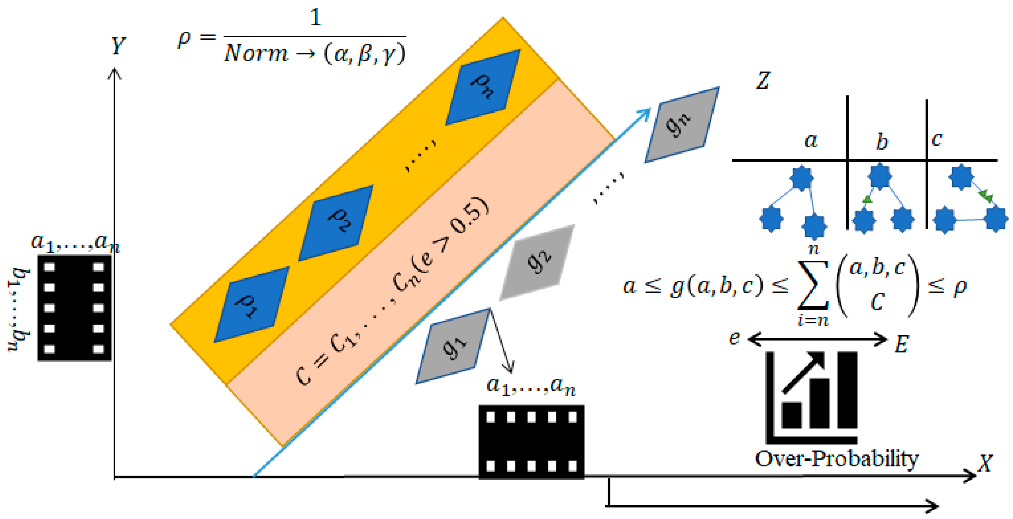
 = g a i n   A   1 , 2 , 3 , 4 , ..... ,   n . As illustrated in Figure 7, we establish the GG to ensure that the LG for every blend reduces the distance between the two triangles in order to create the blend function. Furthermore, Figure 7 also illustrates over-probability stretch using three dimensions. The correlation of the features g , gain function ɀ and over probability ρ can be determined as:
0 g a , b , c   i = 0 n a , b , c C ρ
Overfitness (z) is observed to be reduced in the x and y coordinates. The primary purpose of GG is to maintain the point in the area where the mistake “err” is acceptable.
We tweak the gain function to ensure that in the final blend we may filter the algorithm and progressively blend to be as optimal as is feasible. This is done in considering the fact that LG will be extremely high in lower dimension, and GG designated as ɀ will be lower in lower dimension. As rationally demonstrated in the algorithm formulation, the approximation function (AF) connects the score factor between a collection of predictor characteristics S i n p u t = {1, 2, 3, 4,......, T n } and target variables S o u t p u t = {1, 2, 3, 4,......, T n }. As a result, we compute GG by employing Equations (24)–(28).
= ( L F 1 L F 2 )   N o r m     α , β , γ × e n   1 2   i = 1 m j = 1 m α β γ i , j α i , j , β i , j , γ i , j   + k = 1 K α β γ k

3.4. Final Framework of PTIP

A robust framework that combines hardware, firmware and software optimization is needed to optimize an ML space and algorithm. Several cutting-edge algorithms are utilized to support the software optimization tactics. The final framework is supported by the regularized risk reduction approach and kernel learning in different segments.
Let Ω * , x y z be a convex function for unconstrained minimization of the learning the regularized risk minimization, where space is considered distributed in 3-D dimension, for which our goal is to optimize the algorithm blend in z-dimension with minimum cost function a , b , c , such that the averaged empirical risk function (Φ(t)) associated with algorithm blend inside the boundaries of convex function. Thus, we construct:
Ω * , a b c = Ω * , a b c   F . ρ f A , B , C x x y 2 × y z
To conduct the experiments, typical experimental values for the local gain, global gain, and cost function have been chosen which are provided in Table 4.
Figure 8 depicts the cost function reduction based on LG function. As we can see, LG, based on M.D as constructed earlier in theory, decides the widening or shrinking of the green shape, as shown.
As the arrow moves in the 3-D space (cube) in either direction (optimum for z) then the COST function changes, for which the following conditions apply in optimum space in acceptable Gain function as explained earlier, such that F     min F     R + 1 Φ t , for t     T + 1 R , and R n     R for infinite point in 3-D space.
Finally, we can write the generic form of our three constructs that this theorem aimed to develop. The following algorithm aims to govern these and provides to the external layer that can be built as:
l g o . B l e n d x , y , z ) = i = 0 n e w   N F   i + j = 0 n e w   K j   F   i × j   m , n , o X , Y , Z A m + A n + A 0
E x , y , z = A l g o . E r r o r x , y , z = i = 1 g x , y , z A l g o . G G ( x , y , z j = 1 e r r x , y , z E r r 2   j
The optimization of the model is critical. As a result, there is a requirement for experimental examination of various functions to be employed for improvement, as indicated in Table 5.
Definition 1. 
PTIP explains the principles of the two essential functions of tuning and blending. These constructions proved to be really helpful for classification objectives. Additionally, this definition builds the Binary decomposition function that the LT object uses to define and calculate the cost function.
The Algorithm 3 builds on Theorem 3, which computes the complex error function, gain function, and Blend function. The Algorithm 3 lowers model parameter errors in order to produce a resilient framework. Figure 9 depicts the proposed PTIP at a higher elevation. The framework is an enhancement to the normal machine learning approach for training and assessing raw data. The innovative ideas of LE, GE, LG, and GG are presented in the final framework, which jointly aid in enhancement.
Algorithm 3: Blended and optimal computation for a resilient framework
Input: Φ ,   Risk emp f ,   e ,   E , Ё   , F n , The features set, Data Sets for Sampling
Output: E ,   Algo . Blend x , y , z ), Algo . GG ( x , y , z
Initialization: e     0 ,   E     0
  • Create LTObject, NODES i N , PTIP
  • Generate ObjectIMLE(h)/* Generate an object reference for improved machine learning engine application programming interface (API)*/
  • Set ObjectIMLE.PublicFunctions(h.IMLE, h.EFES, h.EWPM, h.ICCS)/* managing the four constructs*/
  • Compute Global SDE σ     j γ 2 j   n p 1
  • Initialize Y i ,   ϵ
  • For (each row in LTobject) Do
  • Construct: the W from the LT
  • Construct Logical 3D Triangle /* As shown in Figure 7 */
  • Compute LE /*Using equations (19) */
  • While (Distance Function Reduces and E     e   & &   E     0 : 1 ) )   D o
  • Compute E d   x 1 x 2 2 + y 1   y 2 2
  • Compute H d   j = 1 k x j y j
  • Set P Y i =   y i       π i y i 1   π i 1 y i
  • Update LTObject ( E d , H d )
  • If ( E d and H d < W Y i )   ) then
  • Compute: M d   j = 1 k x j y j p 1 p
  • Compute: LG g x , y , z
  • Compute ObjectIMLE.Fitness(g.EFES)
  • Recompute E d and H d /* Based on g.EFES) */
  • Set Norm     α , β , γ
  • Compute
  • End If
  • Compute LF 1   p 1 1 p 1
  • Compute LF 2   p 2 1 p 2
  • Set R n     R
  • Set t     T + 1 R /* T is averaged of t */
  • Set e L , e H x X , y Y , z Z /* Based on LT object values */
  • End While
  • Examine ObjectIMLE.Optimize( LF 1 ,   LF 2 ,   )
  • Update LTObject.Metrics(ObjectIMLE)
  • Compute E ,   Algo . Blend x , y , z ), Algo . GG ( x , y , z
  • End For
  • Return E ,   Algo . Blend x , y , z ), Algo . GG ( x , y , z
Definition 2. 
PTIP includes a thorough explanation of the Cost function theory based on Definition 1. This cost function is also essential for evaluating the algorithms, comparing components and features, as well as for computing the precise quantification of the blending and tuning functions.
Case Study 1. 
The proposed PTIP solves two major issues, weaker generalization and reduced accuracy. The proposed PTIP can be expanded to popular machine learning scenarios. Generalization in machine learning shows how well a trained model categorizes or predicts previously unobserved data. When a machine learning model is generalized, it may be trained to function across all subsets of unknown data. One instance is the intricate clinical processes involved in medication manufacture. Particularly with today’s high-tech treatments dependent on particular ingredients and manufacturing processes, medication creation takes time. The entire process is divided into several stages, some of which are contracted out to specialized suppliers. Therefore, these procedures need to be carried out accurately.
It has currently been observed with COVID-19 vaccine production that it requires generalization. The vaccine’s creators provide the production blueprint, which is then carried out in sterile production facilities. The vaccine is transported in tanks to businesses that fill it in clinical settings in tiny dosages before another business produces the supply. Additionally, medications may only be kept for a short period of time and frequently require particular storage conditions. Accurate treatment should be provided for these disorders. Clinical conditions can be accurately provided by the PTIP. The entire planning process is a very complex process that starts with having the appropriate input materials available at the appropriate time, continues with having enough production capacity, and ends with having the appropriate number of medications stored to meet demand. In addition, this has to be handled for countless treatments, each with a particular set of circumstances. The management of this complexity requires the use of computational approaches. For instance, PTIP with supervised learning techniques is used to choose the best partners for the production process.

4. Experimental Result and Discussion

This section presents various experimental results with necessary discussion and information. Each figure is accompanied with detailed information and comments to elaborate on the experimental analysis of the proposed model.

4.1. Research Methodology and Datasets

4.1.1. Research Methodology

Extensive research, acquaintance, and assessment are critical aspects in establishing the foundation of our proposed PTIP paradigm. As a result, we implemented the proposed PTIP and compared it to existing state-of-the-art algorithms, and as a further result, libraries used for existing algorithms are used for getting the outcomes. For diverse research topics and datasets we investigated the literature and reported their conclusions. Some of the results are compared to our proposed approach, as indicated in the results in the following sections. The goal of our study is to learn the current status of these ML algorithms so that we may progress them with our work, as detailed in this paper. To summarize, the genuine comparison is rather difficult due to the nature of the issue and datasets for which the algorithms are designed. In other words, one may outperform the other in some instances, but the reverse outcomes may be found in others. The scope of this article does not allow for a detailed comparison and experimental examination of each. A broad comparison of several of the algorithms is offered.

4.1.2. Datasets

We made use of information from the following several domains. Some datasets are available in raw, CSV, and SQL light formats, complete with parameters and field descriptions. All of our input data were converted and stored in the SQL Server database system. Some datasets have been discovered to be appropriate for performing tasks such as stock market, healthcare prevention, criminal control prediction, and epidemic identification.
http://www.Kaggle.com, accessed on 1 August 2022. Iris species, credit card fraud detection, flight delays and cancellations, human resource analytics, daily news for market prediction, SMS spam collection, 1.88 Million US wildfires, gender classification, Twitter users, retail data Analytics, US mass shootings, breast cancer, exercise pattern prediction, fatal police shootings, Netflix prize data, student survey, Pima Indians diabetes Database, Zika virus epidemic, WUZZUF Job Posts.
Social networking APIs.
http://snap.standford.edu, accessed on 1 August 2022. Twitter, Facebook, bitcoin and Wiki dataset.
https://aws.amazon.com/datasets/, accessed on 1 August 2022. Japan Census data, Enron email data, 1000 Genomics Project.
http://archive.ics.uci.edu/ml/index.php, accessed on 1 August 2022. heart disease dataset, Iris, car evaluation, bank marketing data.
https://www.reddit.com/r/bigquery/wiki/das, accessed on 1 August 2022.

4.1.3. Tools

The preliminary work is done using a Microsoft SQL Server and machine learning, and Microsoft Azure. The R language, C#, and Python were used to assess the efficacy of the proposed approach and underlying algorithms. Python libraries such as Pandas, SciPy, Matplotlib, Numpy, statsmodels, scikit-learn, fuel, SKdata, ScientificPython, and fuel, mILK have been implemented. Additionally, R libraries such as KlaR, gbm, RWeka, tree, CORELearn, ipred, rpart, MICE Package, CARET, PARTY, and random forest were utilized. Finally, GraphPad Prism is used to generate the simulated findings.
Based on the testing, we obtained the following interesting metrics:
Accuracy with fitness factor;
Relative Accuracy;
PTIP with Fitness function;
Error Reduction;
Generalization measurement.

4.2. Accuracy

We ran 10 experiments (using 200 data samples) for various datasets to observe the overall performance of the algorithms: Support vector machine (SVMs), K-Nearest Neighbor (KNN), Logistic Regression, Multiple Linear Regression (MLR) [29], Decision tree (DR) [30], Graph-based boosting (GB) [31], and Random forest (RF) algorithm [32]. The PTIP is implemented and compared with existing techniques. The results are produced as depicted in Figure 10a. We used CART and ID3 for DT, and it has been observed that the proposed PTIP is found to be efficient. When the number of data samples is increased to more than 300+, the performance of the proposed PTIP still remains stable as compared to competing algorithms depicted in Figure 10b. On the other hand, the accuracy of the contending algorithms is greatly affected. It is imperative to note that we observed through our experiments that the outcome of various algorithms is not highly consistent. Hence, it is our motivation to pursue this research to stabilize the outcome and create a modified version that may be generalizable for many different problems and datasets.

4.3. Relative Accuracy

The relative accuracy shows that the measured value should be almost comparable to the standard value. The proposed method PTIP delivers the optimum fitting. Figure 11a shows how to calculate relative accuracy using error limits reflection. In the case of underfitting, outfitting, and global assessment error, a modest global gain is employed. The proposed PTIP’s performance was compared to the following state-of-the-art methods: an iterative method for discrete variational (IMDV) [20]; cross-modal Turing test (CMTT) [21]; polynomial-time Turing machine (PTTM) [22]; neural Turing machine (NTM) [23]; and a-decidable and i-decidable algorithms (AIA) [24]. According to the experimental data, the PTIP generates the least relative accuracy with error bounds reflection.
The lower relative accuracy with low GG is considered good. The PTIP obtains 38.76% relative accuracy with error bounds reflection. While the contending methods produce 48.7–61.2% relative accuracy with error bounds reflection, that is considered worse. Figure 11b demonstrates the relative accuracy with a high GG. Based on the result, it is observed that PTIP produces better relative accuracy that helps improve the classifier. The main reason for getting better relative accuracy with high GG is to use of improved optimum fitness function. The PTIP obtains 70.5% relative accuracy with high GG, which is considered an acceptable accuracy. On the other hand, the contending methods gain low relative accuracy with high GG which is considered worse. The contending methods obtain 42.4–55.3% relative accuracy with high GG. The findings were derived from 10 separate datasets using an experiment with an average of 20 runs.

4.4. Fitness Process

A fitness function is a type of objective function generated by the proposed PTIP in order to define a single figure of merit. The testing is carried out, and the findings are classified into four colors: in each dimension the blue signifies extreme overfitting.
Green and yellow show that the classifier is unable to distinguish between overfitting and underfitting, while orange shows the best fit. Figure 12a shows the best fitness capability in each dimension. The inaccuracy at the negative value has been noted based on the results. The perfect performance of the LT optimum fitness function is depicted in Figure 12b. The absence of the blue tint is noticeable. Furthermore, it indicates that the z-dimension has the largest convergence, which is preferably required. As a consequence, the data are filtered using PTIP to find the optimal fitness range.

4.5. Error Reduction

The PTIP is capable of reducing errors. The error reduction method is depicted in Figure 13a–d. Figure 13a depicts the gain function dispersed across ten experimental runs. This result shows that the blended function in PTIP is distributed randomly along all axes. It demonstrates that GG is exceedingly low, and the model’s fitness is quite bad. Figure 13b depicts the progress of the PTIP as the number of errors decreases. Figure 13c depicts the tuning process’s evolution. As can be observed, the x and y dimensions have faded, and z has outrun the fitness limitations. However, the yellow color in the z-axis indicates an inaccuracy of more than 80%, which is still unacceptable for model application. Figure 13d finally shows the error in bounds of the (20–80%) rule, and the z-dimension has finally been optimized. The values displayed for 1.0 are optimistic, and the realistic values are observed from ranging 0.6–0.85.

4.6. Generalization Measurement

The generalization measurement process is depicted in Figure 14a–d. The experiment for 200 random datasets has been demonstrated using the proposed PTIP for generalization improvement. The proposed PTIP’s GE and LE functions are depicted. A circle represents the GE function, whereas a square represents the LE function. It should be highlighted that these findings come after measuring the model’s accuracy as an ideal fit across many thousand iterations.
Figure 14a depicts the development of a random distribution of local and global complex error functions. Figure 14b depicts the better separation of the two functions. Figure 14c depicts the model gradually learning (self-teaching) the distinction of LE and GE. Finally, Figure 14d shows the optimal separation of both functions. It should be observed that both functions overlap since one is local and the other is global. It is concluded that the overall generalization is greatly improved.

5. Conclusions and Future Work

This section summarizes the whole outcome of the proposed approach as well as its benefits.

5.1. Conclusions

The parallel Turing integration paradigm is described in this study to facilitate dataset storage. The proposed PTIP approach comprises of three cutting-edge building blocks: (a) it demonstrates the expansion of a logical 3-D cube that administers the algorithms to ensure optimal performance; (b) it demonstrates the improvement in a blend of algorithms based on parallel tuning of model and classifiers; and (c) it provides the ultimate model engineering to learn from its errors (wrong predictions) and explain itself to choose the correct algorithm and eliminate the incorrect predictions.
The outcomes of several tests are discussed in this article. To fine-tune the model and produce simulated data for the study, we ran 10–20 trials. In 3D space, the LG and GG functions have been developed and improved. Finally, the proposed PTIP offered better outcomes with the ability to generalize on a particular collection of facts and issues.

5.2. Future Work

We will test more algorithms, particularly in the fields of unsupervised learning, to enhance the PTIP and its components. We will be improving/developing a model called the “Predicting Educational Relevance For an Efficient Classification of Talent (PERFECT) algorithm Engine” (PAE). The PAE may be used in conjunction with PTIP and includes three cutting-edge algorithms: Good Fit Student (GFS); Noise Removal and Structured Data Detection (NR-SDD); and Good Fit Job Candidate (GFC).

Author Contributions

A.R.: conceptualization, writing, idea proposal, software development, methodology, review, manuscript preparation, visualization, results and submission; M.B.H.F. and M.A. (Mohsin Ali): data curation, software development, and preparation; F.A. and N.Z.J.: review, manuscript preparation, and visualization; G.B., M.A. (Muder Almi’ani), A.A., M.A. (Majid Alshammari) and S.A.: review, data curation and editing. All authors have read and agreed to the published version of the manuscript.

Funding

This work was supported by Taif University Researchers Supporting Project number (TURSP-2020/302), Taif University, Taif, Saudi Arabia.

Data Availability Statement

The data that support the findings of this research are publicly available as indicated in the reference.

Acknowledgments

The authors gratefully acknowledge the support of Mohsin Ali for providing insights.

Conflicts of Interest

The authors declare no conflict of interest.

References

  1. Duan, B.; Yuan, J.; Yu, C.-H.; Huang, J.; Hsieh, C.-Y. A survey on HHL algorithm: From theory to application in quantum machine learning. Phys. Lett. A 2020, 384, 126595. [Google Scholar] [CrossRef]
  2. Ho, S.Y.; Wong, L.; Goh, W.W.B. Avoid oversimplifications in machine learning: Going beyond the class-prediction accuracy. Patterns 2020, 1, 100025. [Google Scholar] [CrossRef] [PubMed]
  3. Razaque, A.; Amsaad, F.; Halder, D.; Baza, M.; Aboshgifa, A.; Bhatia, S. Analysis of sentimental behaviour over social data using machine learning algorithms. In Proceedings of the Advances and Trends in Artificial Intelligence. Artificial Intelligence Practices: 34th International Conference on Industrial, Engineering and Other Applications of Applied Intelligent Systems, IEA/AIE 2021, Kuala Lumpur, Malaysia, 26–29 July 2021; Springer International Publishing: Berlin/Heidelberg, Germany; pp. 396–412. [Google Scholar]
  4. Uddin, M.F.; Rizvi, S.; Razaque, A. Proposing logical table constructs for enhanced machine learning process. IEEE Access 2018, 6, 47751–47769. [Google Scholar] [CrossRef]
  5. Razaque, A.; Ben Haj Frej, M.; Almi’ani, M.; Alotaibi, M.; Alotaibi, B. Improved support vector machine enabled radial basis function and linear variants for remote sensing image classification. Sensors 2021, 21, 4431. [Google Scholar] [CrossRef]
  6. Yang, Y.; Wu, L. Machine learning approaches to the unit commitment problem: Current trends, emerging challenges, and new strategies. Electr. J. 2021, 34, 106889. [Google Scholar] [CrossRef]
  7. Kiselev, P.; Kiselev, B.; Matsuta, V.; Feshchenko, A.; Bogdanovskaya, I.; Kosheleva, A. Career guidance based on machine learning: Social networks in professional identity construction. Procedia Comput. Sci. 2020, 169, 158–163. [Google Scholar] [CrossRef]
  8. Zhao, L.; Ciallella, H.L.; Aleksunes, L.M.; Zhu, H. Advancing computer-aided drug discovery (CADD) by big data and data-driven machine learning modeling. Drug Discov. Today 2020, 25, 1624–1638. [Google Scholar] [CrossRef]
  9. Belmonte, L.; Segura-Robles, A.; Moreno-Guerrero, A.-J.; Parra-González, M.E. Machine learning and big data in the impact literature. A bibliometric review with scientific mapping in Web of science. Symmetry 2020, 12, 495. [Google Scholar] [CrossRef] [Green Version]
  10. Jiang, J. Selection Bias in the Predictive Analytics with Machine-Learning Algorithm. Ann. Emerg. Med. 2021, 77, 272–273. [Google Scholar] [CrossRef]
  11. Lure, A.C.; Du, X.; Black, E.W.; Irons, R.; Lemas, D.J.; Taylor, J.A.; Lavilla, O.; de la Cruz, D.; Neu, J. Using machine learning analysis to assist in differentiating between necrotizing enterocolitis and spontaneous intestinal perforation: A novel predictive analytic tool. J. Pediatr. Surg. 2020, 56, 1703–1710. [Google Scholar] [CrossRef]
  12. Xiong, D.; Fu, W.; Wang, K.; Fang, P.; Chen, T.; Zou, F. A blended approach incorporating TVFEMD, PSR, NNCT-based multi-model fusion and hierarchy-based merged optimization algorithm for multi-step wind speed prediction. Energy Convers. Manag. 2021, 230, 113680. [Google Scholar] [CrossRef]
  13. Lin, S.; Kim, J.; Hua, C.; Park, M.-H.; Kang, S. Coagulant dosage determination using deep learning-based graph attention multivariate time series forecasting model. Water Res. 2023, 232, 119665. [Google Scholar] [CrossRef]
  14. Schorlemmer, M.; Plaza, E. A uniform model of computational conceptual blending. Cogn. Syst. Res. 2021, 65, 118–137. [Google Scholar] [CrossRef]
  15. Messaoud, S.; Bradai, A.; Bukhari, S.H.R.; Qung, P.T.A.; Ahmed, O.B.; Atri, M. A Survey on Machine Learning in Internet of Things: Algorithms, Strategies, and Applications. Internet Things 2020, 12, 100314. [Google Scholar] [CrossRef]
  16. Basha, S.M.; Rajput, D.S. Survey on Evaluating the Performance of Machine Learning Algorithms: Past Contributions and Future Roadmap. In Deep Learning and Parallel Computing Environment for Bioengineering Systems; Academic Press: Cambridge, MA, USA, 2019; pp. 153–164. [Google Scholar]
  17. Gambella, C.; Ghaddar, B.; Naoum-Sawaya, J. Optimization problems for machine learning: A survey. Eur. J. Oper. Res. 2020, 90, 807–828. [Google Scholar] [CrossRef]
  18. Simsekler, M.E.; Rodrigues, C.; Qazi, A.; Ellahham, S.; Ozonoff, A. A comparative study of patient and staff safety evaluation using tree-based machine learning algorithms. Reliab. Eng. Syst. Saf. 2021, 208, 107416. [Google Scholar] [CrossRef]
  19. Tandon, N.; Tandon, R. Using machine learning to explain the heterogeneity of schizophrenia. Realiz. Promise Avoid. Hype. Schizophr. Res. 2019, 214, 70–75. [Google Scholar]
  20. Ferraro, S.J.; de Diego, D.M.; Martín de Almagro, R.T.S. Parallel iterative methods for variational integration applied to navigation problems. IFAC-Pap. 2021, 54, 321–326. [Google Scholar] [CrossRef]
  21. Leshchev, S.V. Cross-modal Turing test and embodied cognition: Agency, computing. Procedia Comput. Sci. 2021, 190, 527–531. [Google Scholar] [CrossRef]
  22. Pinon, B.; Jungers, R.; Delvenne, J.-C. PAC-learning gains of Turing machines over circuits and neural networks. Phys. D Nonlinear Phenom. 2023, 444, 133585. [Google Scholar] [CrossRef]
  23. Faradonbe, S.M.; Safi-Esfahani, F. A classifier task based on Neural Turing Machine and particle swarm algorithm. Neurocomputing 2020, 396, 133–152. [Google Scholar] [CrossRef]
  24. Eberbach, E. Undecidability and Complexity for Super-Turing Models of Computation. Proceedings 2022, 81, 123. [Google Scholar]
  25. Kashyap, K.; Siddiqi, M.I. Recent trends in artificial intelligence-driven identification and development of anti-neurodegenerative therapeutic agents. Mol. Divers. 2021, 25, 1517–1539. [Google Scholar] [CrossRef]
  26. Mohammadi, M.; Rashid, T.A.; Karim, S.H.T.; Aldalwie, A.H.M.; Tho, Q.T.; Bidaki, M.; Rahmani, A.M.; Hoseinzadeh, M. A comprehensive survey and taxonomy of the SVM-based intrusion detection systems. J. Netw. Comput. Appl. 2021, 178, 102983. [Google Scholar] [CrossRef]
  27. Hu, J.; Peng, H.; Wang, J.; Yu, W. kNN-P: A kNN classifier optimized by P systems. Theor. Comput. Sci. 2020, 817, 55–65. [Google Scholar] [CrossRef]
  28. Nabi, M.M.; Shah, M.A. A Fuzzy Approach to Trust Management in Fog Computing. In Proceedings of the IEEE 2022 24th International Multitopic Conference (INMIC), Islamabad, Pakistan, 21–22 October 2022; pp. 1–6. [Google Scholar]
  29. Tang, W.; Li, Y.; Yu, Y.; Wang, Z.; Xu, T.; Chen, J.; Lin, J.; Li, X. Development of models predicting biodegradation rate rating with multiple linear regression and support vector machine algorithms. Chemosphere 2020, 253, 126666. [Google Scholar] [CrossRef]
  30. Zhou, H.F.; Zhang, J.; Zhou, Y.; Guo, X.; Ma, Y. A feature selection algorithm of decision tree based on feature weight. Expert Syst. Appl. 2021, 164, 113842. [Google Scholar] [CrossRef]
  31. Liu, Z.; Jin, W.; Mu, Y. Graph-based boosting algorithm to learn labeled and unlabeled data. Pattern Recognit. 2020, 106, 107417. [Google Scholar] [CrossRef]
  32. Jain, N.; Jana, P.K. LRF: A logically randomized forest algorithm for classification and regression problems. Expert Syst. Appl. 2023, 213, 119225. [Google Scholar] [CrossRef]
Figure 1. Functional components of PTIP for accuracy enhancement.
Electronics 12 01129 g001
Figure 2. Illustration of Internals of the PTIP for preprocessing.
Electronics 12 01129 g002
Figure 3. Illustration of maximum error bounds for risk estimation global function.
Electronics 12 01129 g003
Figure 4. Illustration of risk estimation function in 3-d space for in-bound LE and GE.
Electronics 12 01129 g004
Figure 5. Weight of Global error.
Electronics 12 01129 g005
Figure 6. Logical illustration of complex error function in terms of LE and GE spread in each dimension.
Electronics 12 01129 g006
Figure 7. Blend minimization distance between two triangles using over-probability.
Electronics 12 01129 g007
Figure 8. Cost function reduction using local gain for optimal strategy.
Electronics 12 01129 g008
Figure 9. Illustration of elevated level for proposed PTIP.
Electronics 12 01129 g009
Figure 10. (a) Comparison of PTIP with existing algorithms based on correlation accuracy with fitness factor with 200 data samples; and (b) Comparison of PTIP with existing algorithms based on correlation accuracy with fitness factor with 300+ data samples.
Electronics 12 01129 g010
Figure 11. (a) demonstrates relative accuracy with low GG; and (b) demonstrates relative accuracy with high GG.
Electronics 12 01129 g011
Figure 12. (a) Illustration of a higher diffusion for entire fitness functions, which demonstrates extreme overfitting; (b) shows perfect performance of the LT optimum fitness.
Electronics 12 01129 g012
Figure 13. (a) shows spread of gain function; (b) shows the progress of the PTIP as the number of errors decreases; (c) displays the evolution of turning process; and (d) shows the error optimization process.
Electronics 12 01129 g013
Figure 14. (a) demonstrates the generalization process for the random distribution of local and global complex error functions; (b) demonstrates the enhanced separation of the two functions (LE and GE); (c) demonstrates the self-learning process for the separation of LE and GE; (d) demonstrates the optimal separation of both functions and overlapping of LE and GE.
Electronics 12 01129 g014
Table 1. Contemporary contributions of existing studies.
ApproachesTuring Operations for Machine LearningFeaturesVulnerabilities
IMDV [20]Iterative approach for continuous variational methodsA parallel approach that employs the capabilities of several cores of GPUs (graphics cards) and CPUs (Central processing unit) for addressing the extrapolation problemIts performance is limitted to two applications:a fuel-optimal and navigation problem.
CMTT [21]Cross-modal Turing testing processThe cross-modal Turing test was employed as an all-purpose communication interface for the rapid learning and model adjustment This method could only work for transfer learning.
PTTM [22]Utilization of the polynomial-time Turing machineProjected increases in sample efficiency, offered lower and upper bounds between the intensity of these limitationsIncreased circuit complexity
NTM [23]Neural Turing Machine with a long-term memory,Neural Turing Machine is integrated as a Turing machine with a long-term memory, to carry out variety of simple and sophisticated tasks, including sort, copy, N-gram, etc. Complex jobs, such as classifications The weights of neural Turing machine could not be improved
AIA [24]Introduction of AIA algorithm based on super-Turing modelsApproximate, randomised, and parallel algorithms were used to solve intractable problemsInaccurate for decision-making
Proposed PTIPParallel Turing integration paradigmProposed PTIP is able to quantify the matching, fitness, and accuracy. Furthermore, the proposed PTIP ensures that the model is neither overfit nor biased Trained to be administered by minimum and maximum error bounds
Table 2. Quantified comparison of optimal fitness.
O p . F x O p . F x , y O p . F x , y , z
0.000287230.002387120.03489120
0.2343560.930.87
0.659023+0.73+0.78
Table 3. Shows the results of ten experiments performed on developed functions.
Function12345678910
ψ x 0.01410.01320.02960.09100.13840.27800.46920.59010.62200.6793
ψ y   0.93010.91000.04100.83230.79280.60290.59210.43010.31200.2872
ψ z   0.01300.05700.09620.15020.99910.41700.42880.59190.61290.7709
ψ x , y , z m i n   0.00210.00910.01010.13030.29200.34090.31100.33000.34190.3910
ψ x , y , z m a x   0.54120.59000.60010.64000.64080.66040.69230.71290.70210.7400
The red circled values should be considered as errors that require further investigation.
Table 4. Typical experimental values during training.
MinMaxAveragedOut of Bounds
LG{g(a, b, c)}0.210.720.58−1.8
G G β 0.390.820.72−1.2
a , b , c 0.110.790.63+2.3
Table 5. Experimental analysis of the functions including GG function.
Metrics12345678910
G G 0.01120.03250.03210.07900.13900.20070.38920.58020.64190.6912
Ω * , x y z 0.00120.00240.00790.00830.00970.02930.03010.04020.05110.5990
g x , y , z 0.21980.25000.26980.33120.39000.43190.49010.55100.59120.6339
O.F0.91230.81210.88210.71020.651030.66150.58050.52100.51900.4231
U.F0.70000.68120.66170.61010.55120.51000.49130.43010.41000.3809
Disclaimer/Publisher’s Note: The statements, opinions and data contained in all publications are solely those of the individual author(s) and contributor(s) and not of MDPI and/or the editor(s). MDPI and/or the editor(s) disclaim responsibility for any injury to people or property resulting from any ideas, methods, instructions or products referred to in the content.

