

Data-Driven Constraint Handling in Multi-Objective Inductor Design


Abstract
:1. Introduction
2. Design Procedure of Inductors for DC-DC Converters
3. Statement of the Design Problem
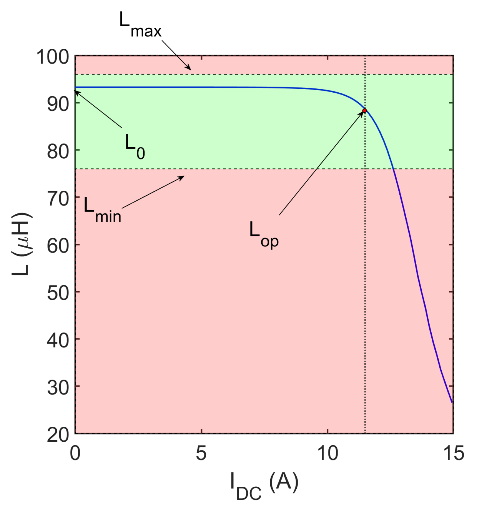
- Lower bound, ;
- Upper bound, ;
- Inductance drop limit, ;
4. Multi-Objective Optimisation Approach
- An outer loop (network), where randomly generated configurations are introduced in the population (exploration);
- An inner loop (clonal selection), where the population is improved by means of local mutations (exploitation).
- Further details about the optimisation algorithm can be found in Appendix A.
- 1.
- First, the geometric consistency is checked (e.g., non-negative area of the core’s windows). An inconsistent configuration is discarded and replaced by a new one if it was randomly generated. Otherwise, if the configuration is a clone (mutated from a feasible configuration), the mutation is gradually reduced until the solution is feasible again.
- 2.
- 3.
- The remaining candidate solutions are evaluated in terms of objectives (volume and total losses).
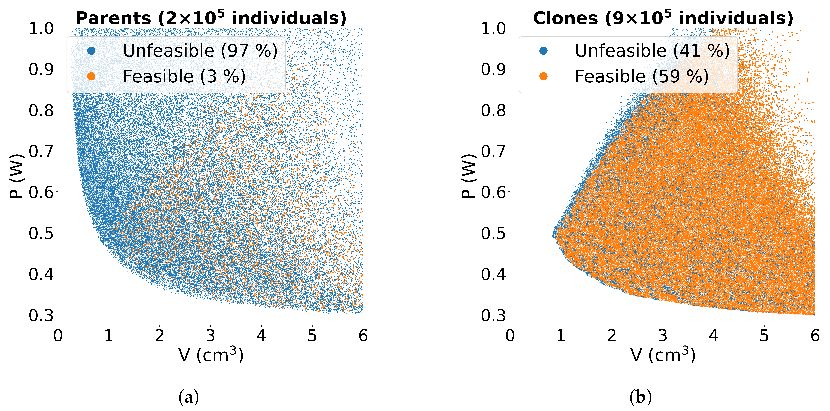
- The clouds of points in Figure 4 represent all the design configurations explored during a complete run of the optimisation procedure on the test problem, in the objectives space (volume V and total losses P, on the x and y axes, respectively). The colour depends on the feasibility of the configurations and distinguishes those configurations compliant with the design constraints (i.e., good, orange points) from those that are unfeasible (i.e., bad, blue points). Two graphs are reported to further distinguish between parent configurations (Figure 4a) and clones (Figure 4b). It can be noticed that only a small percentage of the configurations generated randomly (parents) is feasible. Clones, instead, have higher chances of complying with the design constraints since they originate from local mutations of feasible configurations.
5. Surrogate Modelling of Constraints for Pre-Selection
5.1. AIS-Based Classifier
5.2. Effects of the Classifier on the Optimisation
- True positives: feasible configurations that are correctly classified as positive.
- False positives: unfeasible configurations wrongly classified as positives. Since they are evaluated with the FP during the optimisation, the incorrect classification implies unnecessary calculation that slows down the procedure.
- True negatives: unfeasible configurations correctly classified as negative, which can be correctly disregarded in the optimisation process.
- False negatives: feasible configurations wrongly classified as negatives, which are therefore disregarded during the optimisation. This is the worst case since it implies discarding solutions potentially belonging to the Pareto Front.
5.3. Evaluation of the Classifier’s Performance
- The high percentage of true negatives (around 97%) in the randomly generated configurations considerably reduces the number of FP evaluations in this phase. Despite the high rate of false positives, the low number of total positives identified by the classifier among the parent results in a significant reduction in the unnecessary evaluations of the FP.
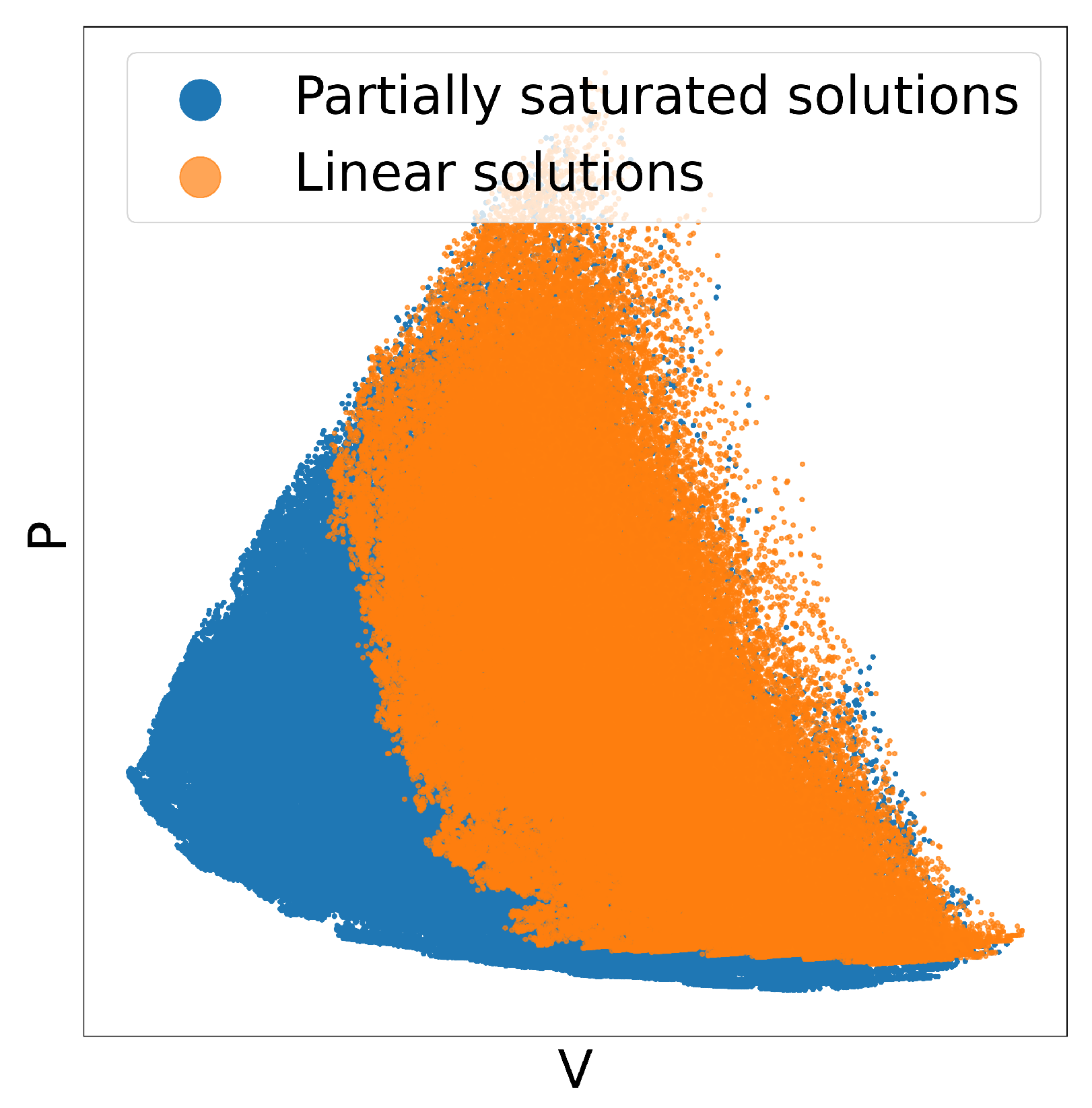
- The good performance in the classification of negatives among parents is motivated by the presence of wide areas of unfeasible configurations in the design space (Figure 5a).
- As previously discussed (Figure 5b), the classification task is much harder in the proximity of the interface between the feasibility region and the rest of the design space. Most configurations generated from local mutations are located in this area. This explains the poor performance of the classifier in the clones. In particular, while around 200,000 FP evaluations are saved by correct classification of unfeasible configurations (true negatives), an equivalent number of feasible configurations are wrongly disregarded.
- The percentage of false positives in clones is smaller than in parents. However, around 150,000 configurations are unnecessarily evaluated.
6. Evaluation of the Surrogate Modelling Approach
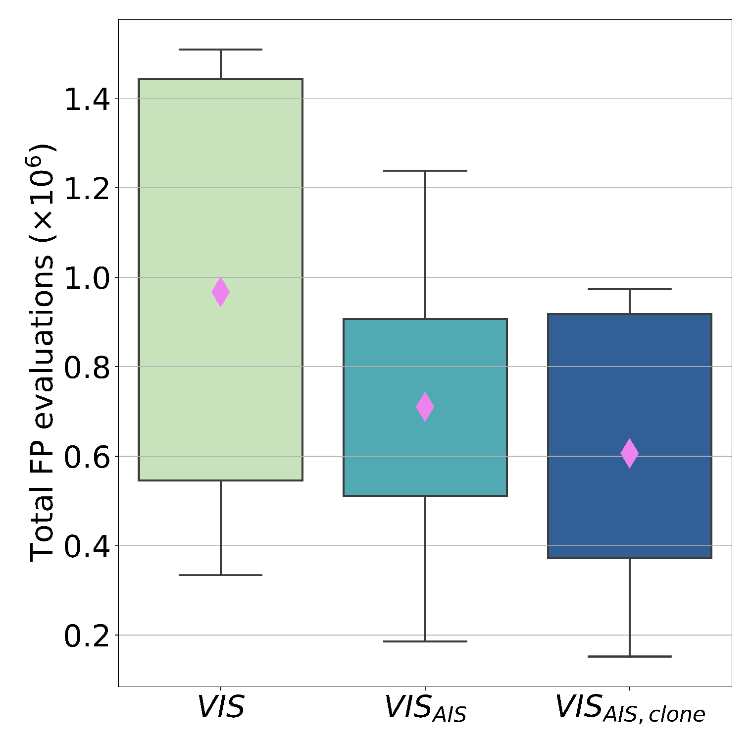
- Execution of VIS optimisation method without a classifier ().
- Application of the classifier only on randomly generated configurations ().
- Application of the classifier both on randomly generated and locally mutated configurations. ().
- For each of the presented cases, 30 optimisation executions are performed. The first result is the average number of FP evaluation calls, reported in Figure 7, in which separated results are reported for the classification of parents and clones.
7. Conclusions
Author Contributions
Funding
Conflicts of Interest
Appendix A
- 1.
- An initial population of configurations (antibodies ) is randomly generated.
- 2.
- A memory set is also created, initially empty, where all the non-dominated solutions found during the search are stored.
- 3.
- The memory set is built through a network loop, where for iterations or until a stop criterion is reached:
- (a)
- The fitness f of all antibodies in the current population is evaluated, also including the antibodies eventually present in the memory set.
- (b)
- The current population is improved through a clonal selection loop, where for iterations or until a stop criterion is reached:
- i.
- The antibodies in the current population (parents) are replicated into clones;
- ii.
- Each clone is then locally mutated. The random mutation is evaluated as follows: , where is a mutation amplitude parameter and f the fitness of the parent (lower fitness corresponds to larger mutations);
- iii.
- The fitness of the clones is evaluated, also including the antibodies eventually present in the memory set;
- iv.
- The clone with the highest fitness is selected and it replaces the parent in the next generation if it has higher fitness.
- (c)
- The current population and the memory set are merged and their affinity is calculated.
- (d)
- Network selection is performed, removing antibodies with high affinity. The affinity threshold is evaluated as follows: , where m is the number of objectives and is the desired size of the memory set.
- (e)
- The memory set is updated with the non-dominated solutions, among those that survived the network selection.
- (f)
- A fraction (with respect to the current size of the population) of randomly generated new configurations is introduced in the population to increase the exploration of the design space.
- 4.
- The final memory set is taken as the Pareto set of the problem.
- The values of the parameters adopted in all the runs of the VIS optimisation are shown in Table A1.

| Parameter | Value |
|---|---|
| Initial population size, | 50 |
| Number of clones, | 5 |
| Desired size of the memory set, | 100 |
| Number of network loops, | 50 |
| Number of clonal selection loops, | 10 |
| Mutation amplitude factor, | 0.02 |
| Fraction of new antibodies, | 0.4 |
References
- Rashid, M.H. (Ed.) Power Electronics Handbook, 4th ed.; Energy Engineering and Power Technology, Butterworth-Heinemann, an imprint of Elsevier: Amsterdam, The Netherlands, 2018. [Google Scholar]
- Hurley, W.G.; Wölfle, W.H. Transformers and Inductors for Power Electronics: Theory, Design and Applications; Reprinted with Corrections ed.; Wiley: Chichester, UK, 2014. [Google Scholar]
- McLyman, C.W.T. Transformer and Inductor Design Handbook, 4th ed.; CRC Press: New York, NY, USA, 2017. [Google Scholar] [CrossRef]
- Hurley, W.G.; Duffy, M.C.; Acero, J.; Ouyang, Z.; Zhang, J. 17—Magnetic Circuit Design for Power Electronics. In Power Electronics Handbook, 4th ed.; Rashid, M.H., Ed.; Butterworth-Heinemann: Oxford, UK, 2018; pp. 571–589. [Google Scholar] [CrossRef]
- Biela, J.; Badstuebner, U.; Kolar, J.W. Impact of Power Density Maximization on Efficiency of DC–DC Converter Systems. IEEE Trans. Power Electron. 2009, 24, 288–300. [Google Scholar] [CrossRef]
- Mühlethaler, J. Modeling and Multi-Objective Optimization of Inductive Power Components. Ph.D. Thesis, ETH Zurich, Zürich, Switzerland, 2012. [Google Scholar] [CrossRef]
- Calderon-Lopez, G.; Scoltock, J.; Wang, Y.; Laird, I.; Yuan, X.; Forsyth, A.J. Power-Dense Bi-Directional DC–DC Converters With High-Performance Inductors. IEEE Trans. Veh. Technol. 2019, 68, 11439–11448. [Google Scholar] [CrossRef]
- Guillod, T.; Papamanolis, P.; Kolar, J.W. Artificial Neural Network (ANN) Based Fast and Accurate Inductor Modeling and Design. IEEE Open J. Power Electron. 2020, 1, 284–299. [Google Scholar] [CrossRef]
- Kaiser, J.; Dürbaum, T. An Overview of Saturable Inductors: Applications to Power Supplies. IEEE Trans. Power Electron. 2021, 36, 10766–10775. [Google Scholar] [CrossRef]
- Milner, L.; Rincón-Mora, G.A. Small saturating inductors for more compact switching power supplies. IEEJ Trans. Electr. Electron. Eng. 2012, 7, 69–73. [Google Scholar] [CrossRef]
- Musumeci, S.; Solimene, L.; Ragusa, C.S. Identification of DC Thermal Steady-State Differential Inductance of Ferrite Power Inductors. Energies 2021, 14, 3854. [Google Scholar] [CrossRef]
- Scirè, D.; Lullo, G.; Vitale, G. Non-Linear Inductor Models Comparison for Switched-Mode Power Supplies Applications. Electronics 2022, 11, 2472. [Google Scholar] [CrossRef]
- Di Capua, G.; Femia, N.; Stoyka, K. Validation of inductors sustainable-saturation-operation in switching power supplies design. In Proceedings of the 2017 IEEE International Conference on Industrial Technology (ICIT), Toronto, ON, Canada, 22–25 March 2017; pp. 242–247. [Google Scholar] [CrossRef]
- Martins, S.; Seidel, A.R.; Perdigão, M.S.; Roggia, L. Core volume reduction based on non-linear inductors for a PV DC–DC converter. Electr. Power Syst. Res. 2022, 213, 108716. [Google Scholar] [CrossRef]
- Gareau, J.; Emadi, A.; Bilgin, B. Power Inductor Optimization Using Non-linear Magnetization Characteristics. In Proceedings of the 2020 IEEE Transportation Electrification Conference & Expo (ITEC), Chicago, IL, USA, 23–26 June 2020; pp. 992–999. [Google Scholar] [CrossRef]
- Sudhoff, S.D. Power Magnetic Devices: A Multi-Objective Design Approach, 2nd ed.; IEEE Press Series on Power and Energy Systems; Wiley: Hoboken, NJ, USA, 2022. [Google Scholar]
- Wang, X.; Zeng, H.; Gunasekaran, D.; Peng, F.Z. Multi-objective design and optimization of inductors: A generalized software-driven approach. In Proceedings of the 2016 IEEE 17th Workshop on Control and Modeling for Power Electronics (COMPEL), Trondheim, Norway, 27–30 June 2016; pp. 1–7. [Google Scholar] [CrossRef]
- Cale, J.; Sudhoff, S.D.; Chan, R.R. Ferrimagnetic Inductor Design Using Population-Based Design Algorithms. IEEE Trans. Magn. 2009, 45, 726–734. [Google Scholar] [CrossRef]
- Wallmeier, P. Pre-optimization of linear and nonlinear inductors using area-product formulation. In Proceedings of the Conference Record of the 2002 IEEE Industry Applications Conference, 37th IAS Annual Meeting (Cat, No.02CH37344), Pittsburgh, PA, USA, 13–18 October 2002; Volume 4, pp. 2445–2450. [Google Scholar] [CrossRef]
- Stratta, A.; Gottardo, D.; di Nardo, M.; de Lillo, L.; Empringham, L.; Espina, J.; Johnson, M. Automated design of integrated inductive components for DC-DC converters. In Proceedings of the 2021 IEEE Design Methodologies Conference (DMC), Bath, UK, 14–15 July 2021; pp. 1–6. [Google Scholar] [CrossRef]
- Solimene, L. Investigation of Inductive Components for Power Electronics Applications. Ph.D. Thesis, Politecnico di Torino, Torino, Italy, 2022. [Google Scholar]
- Solimene, L.; Ragusa, C.S.; Musumeci, S. The role of materials in the optimal design of magnetic components for DC–DC converters. J. Magn. Magn. Mater. 2022, 564, 170038. [Google Scholar] [CrossRef]
- Chiampi, M.; Chiarabaglio, D.; Repetto, M. An accurate investigation on numerical methods for nonlinear magnetic field problems. J. Magn. Magn. Mater. 1994, 133, 591–595. [Google Scholar] [CrossRef]
- Reinert, J.; Brockmeyer, A.; De Doncker, R. Calculation of losses in ferro- and ferrimagnetic materials based on the modified Steinmetz equation. IEEE Trans. Ind. Appl. 2001, 37, 1055–1061. [Google Scholar] [CrossRef]
- Li, J.; Abdallah, T.; Sullivan, C. Improved calculation of core loss with nonsinusoidal waveforms. In Proceedings of the Conference Record of the 2001 IEEE Industry Applications Conference, 36th IAS Annual Meeting (Cat, No.01CH37248), Chicago, IL, USA, 30 September–4 October 2001; Volume 4, pp. 2203–2210. [Google Scholar] [CrossRef]
- Muhlethaler, J.; Biela, J.; Kolar, J.W.; Ecklebe, A. Core Losses Under the DC Bias Condition Based on Steinmetz Parameters. IEEE Trans. Power Electron. 2012, 27, 953–963. [Google Scholar] [CrossRef]
- OCLC: 1197739030; Ferrite Cores. Guidelines on Dimensions and the Limits of Surface Irregularities. Part 8. British Standards Institution: London, UK, 2019.
- Freschi, F.; Repetto, M. Multiobjective Optimization by a Modified Artificial Immune System Algorithm. In Proceedings of the Artificial Immune Systems; Lecture Notes in Computer Science; Jacob, C., Pilat, M.L., Bentley, P.J., Timmis, J.I., Eds.; Springer: Berlin/Heidelberg, Germany, 2005; pp. 248–261. [Google Scholar] [CrossRef]
- Freschi, F.; Repetto, M. VIS: An artificial immune network for multi-objective optimization. Eng. Optim. 2006, 38, 975–996. [Google Scholar] [CrossRef]
- Deb, K.; Pratap, A.; Agarwal, S.; Meyarivan, T. A fast and elitist multiobjective genetic algorithm: NSGA-II. IEEE Trans. Evol. Comput. 2002, 6, 182–197. [Google Scholar] [CrossRef]
- Dudek, G. An Artificial Immune System for Classification With Local Feature Selection. IEEE Trans. Evol. Comput. 2012, 16, 847–860. [Google Scholar] [CrossRef]


| Input voltage | 48 V |
| Output voltage | 24 V |
| Output current | 10 A |
| Maximum current ripple (pp) | 30% |
| Switching frequency | 50 kHz |
| Inductance value | 80 μH |
| Variable | Lower Bound | Upper Bound |
|---|---|---|
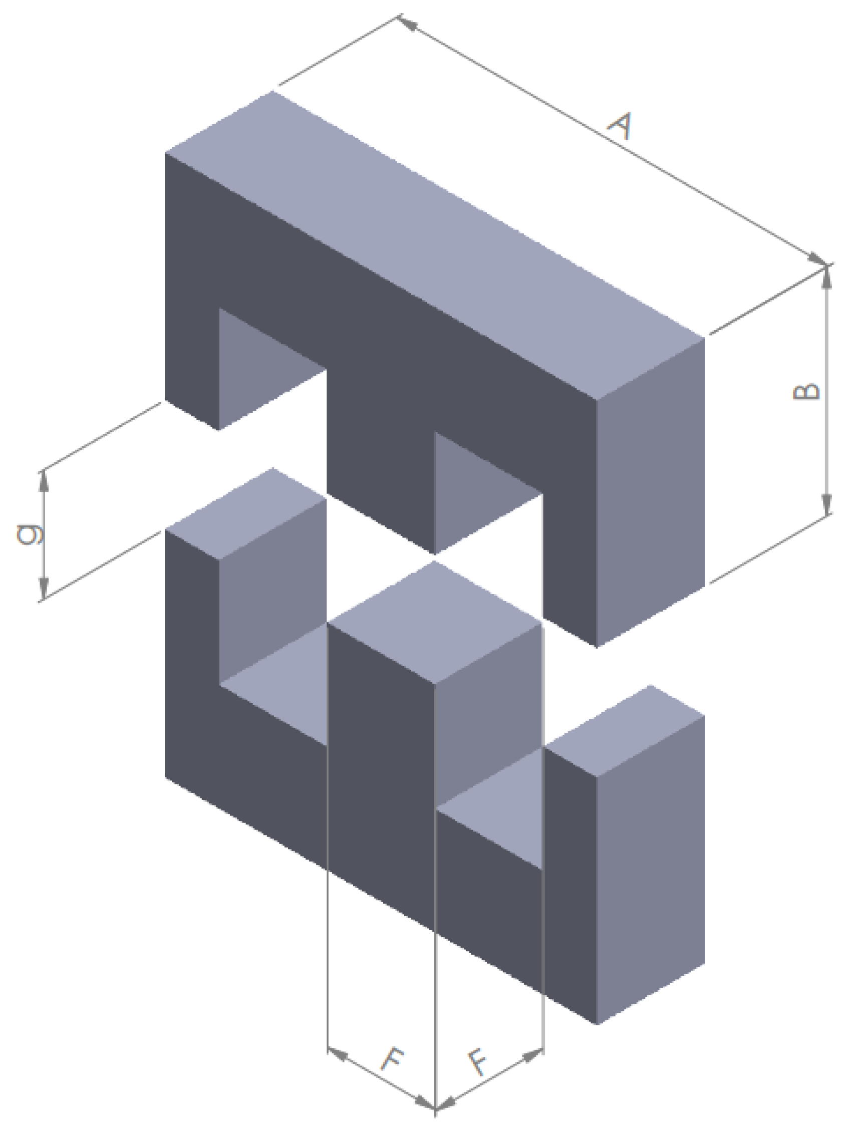
| A | 30 mm | 59.2 mm |
| B | 8 mm | 22.3 mm |
| F | 2 mm | 8 mm |
| g | 0 mm | 2 mm |
| N | 6 | 100 |
| Minimum inductance value, | |
| Maximum inductance value, | |
| Maximum inductance drop factor, | |
| Maximum over-temperature, |
| Parents | Clones | |
|---|---|---|
| True positive (%) | 44 | 67 |
| False positive (%) | 56 | 33 |
| True negative (%) | 99 | 51 |
| False negative (%) | 1 | 49 |
| Total positive | ||
| Total negative |
Disclaimer/Publisher’s Note: The statements, opinions and data contained in all publications are solely those of the individual author(s) and contributor(s) and not of MDPI and/or the editor(s). MDPI and/or the editor(s) disclaim responsibility for any injury to people or property resulting from any ideas, methods, instructions or products referred to in the content. |
© 2023 by the authors. Licensee MDPI, Basel, Switzerland. This article is an open access article distributed under the terms and conditions of the Creative Commons Attribution (CC BY) license (https://creativecommons.org/licenses/by/4.0/).
Share and Cite
Lorenti, G.; Ragusa, C.S.; Repetto, M.; Solimene, L. Data-Driven Constraint Handling in Multi-Objective Inductor Design. Electronics 2023, 12, 781. https://doi.org/10.3390/electronics12040781
Lorenti G, Ragusa CS, Repetto M, Solimene L. Data-Driven Constraint Handling in Multi-Objective Inductor Design. Electronics. 2023; 12(4):781. https://doi.org/10.3390/electronics12040781
Chicago/Turabian StyleLorenti, Gianmarco, Carlo Stefano Ragusa, Maurizio Repetto, and Luigi Solimene. 2023. "Data-Driven Constraint Handling in Multi-Objective Inductor Design" Electronics 12, no. 4: 781. https://doi.org/10.3390/electronics12040781
APA StyleLorenti, G., Ragusa, C. S., Repetto, M., & Solimene, L. (2023). Data-Driven Constraint Handling in Multi-Objective Inductor Design. Electronics, 12(4), 781. https://doi.org/10.3390/electronics12040781