Using a Light-Weight CNN for Perfume Identification with An Integrated Handheld Electronic Nose

Abstract

Exposing counterfeit perfume products is significant for protecting the legal profit of genuine perfume manufacturers and the health of perfume consumers. As a holistic solution to the problem of perfume identification (PI) using an electronic nose (EN), the methods based on convolutional neural network (CNN) simplifies the inconvenient selection of methods and parameter values, which has traditionally complicated existing combinatory methods. However, existing CNN methods that can be used for EN-based PI were designed on the premise that the CNN model can be trained with plenty of computational resources in divide-body ENs. Aiming at PI with an integrated handheld EN, a novel light-weight CNN method, namely LwCNN, is presented for being entirely conducted on a resource-constrained NVDIA Jetson nano module. LwCNN utilizes a sequenced stack of two feature flattening layers, two one-dimensional (1D) convolutional layers, a 1D max-pooling layer, a feature dropout layer, and a fully connected layer. Extensive real experiments were conducted on an integrated handheld EN to the performance of LwCNN with those of four existing benchmark methods. Experimental results show that LwCNN obtained an average identification accuracy of 98.35% with model training time of about 26 s.

1. Introduction

Nowadays, the consumption of perfume products is getting more and more popular, which has promoted the development of the perfume industry. Genuine perfume products of famous brands are commonly produced using confidential professional techniques with selected ingredients. The high profits brought by genuine perfume products stimulated unscrupulous businessmen to counterfeit them with cheap and even noxious ingredients [1]. The existence of counterfeit perfume products not only affected the legal income of genuine perfume manufacturers, but also harmed the health of perfume consumers. However, since the scents in perfume products interact naturally by synergism, compensation, and masking [2], it is hard to expose counterfeit perfume by solely using the human nose. To reliably identify the accurate perfume type, it is necessary to consult specifically designed electronic techniques. Moreover, portable and integrated PI solutions, which bring about high efficiency and great convenience, are significant for real applications.

Existing electronic techniques that can be used for PI mainly include EN [3,4], fluctuation-enhanced sensing (FES) [5,6], gas chromatography (GC) [7], and GC with mass spectrometry (GC-MS) [8,9]. Typical ENs are mainly composed of the measurement acquisition hardware and data processing software. The measurement acquisition hardware comprises the gas route and electronic components. Commonly, the gaseous perfume samples are guided towards the mounted gas sensors. Then, the sensing data of the gas sensors is denoised and stored. Based on the denoised sensing measurements, the perfume type is identified by the data processing software [3]. In contrary to ENs, FES exploits the information contained in the low measurement noises [5] or micro-fluctuations of measurements [5,6]. Typically, the low measurement noises are successively processed with a band-pass filter and an amplifier. Based on the processed data, FES signature spectrums can be calculated by multiplying the normalized power spectral density and the frequency. In the FES mode, multiple different gases can be identified based on the measurements of only one sensor [5]. However, compared with the acquisition of denoised measurements in EN systems, the extraction of low measurement noises in FES methods is more difficult and cost-consuming. GC and GC-MS utilize the standard carrier gas stored in large gas cylinders to drive the gas sample through the chromatographic column. Apart from identifying the perfume type, GC and GC-MS can also separate the different perfume ingredients. Nevertheless, the high cost and large volume of GC and GC-MS stagnate their portable on-site usage. In comparison, EN is relatively more cost-effective and portable. Although existing EN solutions have rarely been reported separating the gaseous ingredients, the gas identification capability of ENs can help in exposing counterfeit perfume products. For example, the integrated handheld EN designed in the author’s laboratory, namely SMUENOSEv2, which utilizes an embedded NVIDIA Jetson nano module as the computation kernel, is suitable for quick on-site PI applications [3].

To improve the PI performance, it is important to design accurate and time-efficient EN-based PI methods. Conventional combinatory EN-based PI methods [4,10,11,12,13] involve the combination of multiple successive steps. The raw measurements are first preprocessed to remove the baseline value and noises. Based on the preprocessed measurements, a set of features are generated by normalization, differentiation, and/or integral operations. The dimension of generated features is then reduced by using the feature extraction methods, such as, principal component analysis (PCA) [14], local linear embedding [15], maximally collapsing metric learning [16], and so on. Finally, the features with reduced dimension are classified using machine learning methods, such as support vector machine [17], back-propagation neural network (BPNN) [18], extreme gradient boosting (XGBoost) [19], light gradient boosting machine (LightGBM) [20], and so on. The perfume type can be identified according to the feature classification result. For each of the above-mentioned steps, there are multiple candidate methods can be selected. Different combinations of selected methods can cause significantly different PI results. The complicated selection process of constituent methods and parameter values influences the time-efficiency and reliability of conventional combinatory methods.

During the past decades, the investigation on deep learning for image classification has aroused worldwide interest [21], which also induced the implementation of deep learning for EN-based PI applications. Unlike conventional combinatory methods, deep learning methods incorporate the processes of feature generation, extraction, and classification. In the deep learning research field, one of the representative methods is the CNN method. LeCun et al. proposed the LeNet for document recognition [22], which can be considered as the seminal work of CNN. Afterwards, multiple of improved CNN methods, such as, AlexNet [23], VGGNet [24], GoogleNet [25], ResNet [26], and so on, were presented for image classification. Inspired by these works, a few CNN models were proposed for solving the EN-based PI problem. To realize gas classification, Peng et al. proposed a very deep CNN with 38 constituent layers, namely GasNet [27], which mainly comprises six convolution blocks of multiple layers, a global average pooling layer, and a fully connected layer. Syuan et al. [28] proposed to transfer the gas measurements to feature map images, which are then processed using a deep CNN with seven convolution blocks of three layers, a global averaging pooling layer, and a fully connected layer. Wang et al. [29] presented a dense CNN, which comprises multiple alternating pairs of dense and transition blocks, to process the EN’s data for identifying the age of mature vinegar. Each of the employed dense and transition blocks are composed of multiple layers. In these works, the computation kernels used for training the CNN models were not detailed. Although all these works utilized deep CNN models, whether a shallow or not very deep CNN model can obtain satisfactory EN-based PI performance needs further investigation. Moreover, with the integrated handheld SMUENOSEv2, the CNN model should be trained on the resource-limited NVIDIA Jetson nano module. For quick on-site EN-based PI, it is necessary to restrict the number of layers in the CNN model.

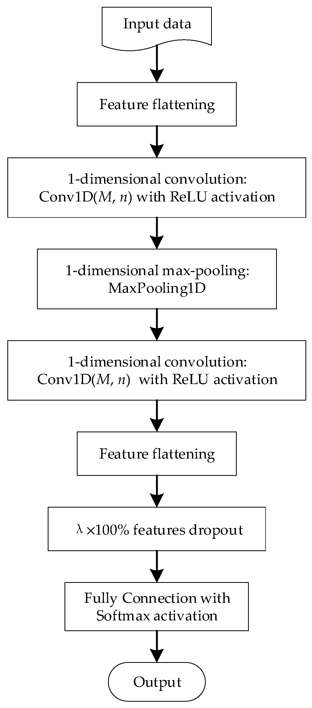
In this paper, a light-weight CNN model, namely LwCNN, is presented for solving the PI problem based on the SMUENOSEv2 platform. Considering the limited computational resource, LwCNN only utilizes two 1D convolutional layers with activation, two feature flattening layers, a 1D max-pooling layer, and a fully connected layer with activation. Among the constituent layers of LwCNN, only the convolutional layers and the fully connected layer contain several trainable weights. Moreover, LwCNN incorporates the sub-processes of feature generation, extraction, and classification, which means the complicated selection of methods and parameter values for these sub-processes are simplified. To comprehensively evaluate the performance of LwCNN, four benchmark methods, those are, XGBoost, LightGBM, BPNN, and GasNet, were compared with LwCNN in extensive real experiments. The novelties of this paper mainly comprise three parts. First, LwCNN employs a feature flattening layer as its first layer, which concatenates the preprocessed measurements of different sensors into a 1D vector. The 1D vector incorporates the information within the junction sections of data sensed by different sensors, which inspired the utilization of 1D convolutional and max-pooling layers. Second, the disposition scheme of the selected constituent layers in LwCNN is novel. The performance of a CNN model is dominated by the selection and disposition of its constituent layer. Third, the experimental PI results of LwCNN obtained on an integrated handheld EN platform are novel. Especially, the evaluated influence of CNN parameters, such as convolution kernel number and length, the dropout proportion, on the PI performance has rarely been studied.

The rest of this paper is organized as follows. In Section 2, the conventional process of EN-based PI is introduced. Section 3 details the operations in LwCNN. Section 4 introduces the experimental setup. The experimental results are detailed and discussed in Section 5. Section 6 concludes the whole paper.

2. Conventional Process of EN-Based PI

To make the EN-based PI methods more understandable, the employed EN platform is briefly sketched first. Figure 1 shows the architecture of the employed integrated handheld EN, namely SMUENOSEv2, which comprises two main types of components: the gas route and electronic components.

At the beginning of each sampling cycle, the perfume samples were dripped into the volatilization pot. Fast airflow was generated by the air pump, and then, guided to accelerate the volatilization of the perfume samples. Then, the volatilized gaseous perfume was carried towards the three-way valve. By controlling the three-way valve, the gas route at the downflow side of the volatilization pot can be switched between the sub-routes 1 and 2, which are timely switched to activate the sampling and washing modes. Once the gas route 1 was switched on, the gaseous perfume was carried towards the gas chamber, which means the gas sensors were exposed in the gaseous perfume. Thus, the three-way valve can be timely switched to control the exposure time of the gas sensors. During the exposure time, the sensing voltages were sampled using AD7606 and STM32. The sampling data was then transmitted from the STM32 to the NVIDIA Jetson Nano module, on which the PI methods were conducted to complete the EN-based PI task.

Conventional combinatory EN-based PI methods comprise multiple successive steps: data preprocessing, feature generation, feature dimension reduction, and feature classification. For each step, there are multiple candidate methods can be selected to complete the corresponding task. For each candidate method, multiple hyperparameters should be tuned to improve the PI performance. Different combinations of methods and parameter values can severely influence the final PI performance [4,30].

Data preprocessing aims to reduce the influence of measurement noises and gas residuals within the EN’s gas route. For filtering the measurement noises, the wavelet denoising method was employed. In the author’s previous work, it has been proven that the wavelet denoising method are capable of filtering out most spiky noises. Subsequently, a baseline subtraction operation was conducted to inhibit the influence of gas residuals within the EN. The term ‘baseline’ means the sensing voltages measured before the gas sensors were exposed in the gaseous perfume. The baseline voltages were mainly caused by the gas residuals left over during the former inexhaustive washing cycle, since the working mode of SMUENOSEv2 can be consecutively switched between the sampling and washing modes.

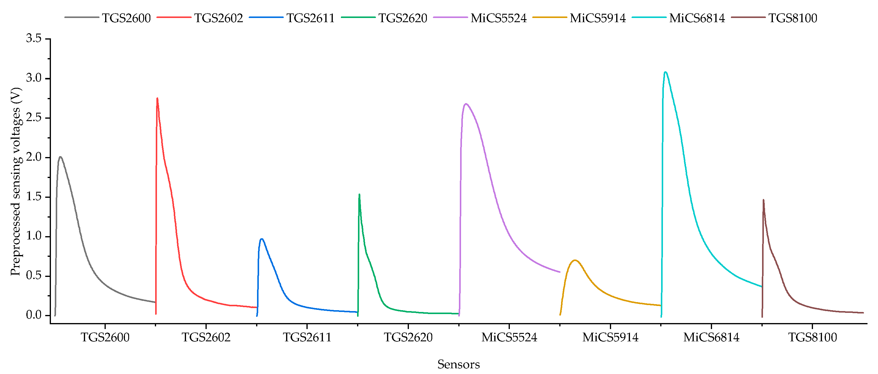
After data preprocessing, the data dimension was still retained at a high value. Due to the curse of dimensionality, directly conducting feature classification with the preprocessed data is time consuming. To generate the features for further classification, multiple statistics were calculated, including normalized peak of the sensing value, normalized time when the voltage peak appeared, final falling proportion, falling proportion at 10 s after the maximum sensing value, and normalized time when the first-order derivative reached the maximum value. Due to the metal oxide semiconductor sensors used in our EN, the sampled sensing voltages demonstrate a fast rising and relatively slow recovery dynamics. It is expected that the generated features are capable of characterizing the dynamics of the sampling data, and thus, contain distinctive information that can be used for further classification. Typically, further feature extraction or dimension reduction was also required. PCA can be used to extract the principal components with lower dimensions as the final features.

Finally, the generated features with reduced dimension were classified to complete the PI task. As three conventional EN-based PI methods, BPNN, XGBoost, and LightGBM methods were separately used as the benchmark methods for feature classification. BPNN is the canonical form of neural network. XGBoost and LightGBM are two improved implementation forms of the gradient-boosting decision tree method, in which the results of multiple decision trees are ensembled to form a better result. According to the author’s previous works [4], XGBoost outperformed other tested methods in terms of mean identification accuracies, while LightGBM obtained similar identification accuracies with relatively higher time-efficiencies.

3. Light-Weight CNN for EN-Based PI

Figure 2 shows the architecture of LwCNN. The main operations of LwCNN comprise a sequence of operation layers. Due to the different gas residuals left over in the EN’s inner space, a baseline subtraction was employed to preprocess the raw measurements. The preprocessed measurements were used as the input of LwCNN. Then, the output of each individual layer is considered as the input of its below layer. Unlike the multiple separated algorithms successively employed in conventional combinatory methods, the operation layers in LwCNN are connected with each other to construct a single network-shaped algorithm.

The operations in the layers of LwCNN are detailed as follows.

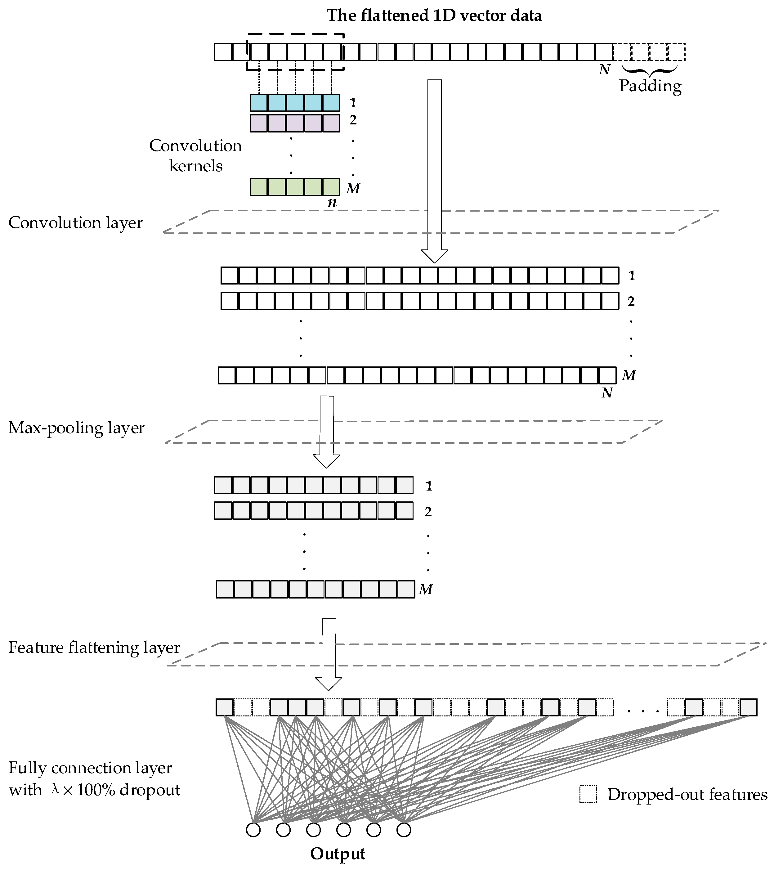
• Feature flattening

As shown in Figure 2, the input data was first processed with the feature flattening operation, in which the preprocessed measurements of the eight different gas sensors were concatenated with each other in a one-by-one manner. In consequence, a 1D vector data was constructed based on the sampling data obtained with an individual perfume sample in each sampling cycle. The 1D vector data inspired the usage of the 1D convolution kernel in the subsequent layer.

2.

1D convolution

The defining characteristic of a 1D convolutional layer is that the dimension of the utilized convolution kernel is one. As illustrated in Figure 3, the length of input vector, the number of convolution kernels, and the length of each convolution kernel are denoted as N, M, and n, respectively. In the 1D convolution operation, each convolution kernel is used to generate a new intermediate vector, which is also called tensor. A total of M tensors or vectors are generated with the M convolution kernels.

Figure 3 illustrates the case that n equals 5. In specific, as indicated by the dashed rectangle in Figure 3, a set of five successive elements of the input data are selected as the factor. A point multiplication between the selected factor and the convolution kernel is conducted. The result of the point multiplication is recorded as one element of the newly generated tensor. As the dashed rectangle moves from the left beginning to right end of the input vector, multiple factors are selected to activate multiple times of point multiplication with the convolution kernel, which result in multiple elements to form the new tensor. To generate a new tensor with the same length as the input vector, four random elements are padded at the end of the input vector. With the padding operation, a total of N factors are selected, and a tensor with the length of N is generated with each convolution kernel.

3.

Activation

Each convolutional layer is followed with an activation operation. In the activation operation, all elements in the tensor are separately substituted into a transfer function. An individual result is generated by the transfer function with each element in the tensor. The results are combined to form a new tensor. Thus, the tensor length is kept invariant in the activation layer.

There are two different types of activation operations used in LwCNN. As shown in Figure 2, the activation functions used after the convolutional layer and the fully connected layer are the ReLU function and the Softmax function, respectively. The ReLU function replaces the negative elements in the tensors with zero-value elements, which can be represented as follows.

$$f\left(x_i\right)=\max \left(x_i,0\right)$$

(1)

The Softmax function, which maps the value of multiple elements into probability values within the range (0, 1), can be represented as follows.

$$f\left(x_i\right)=\frac{e^{x_i}}{{{\displaystyle \sum }}_i{e}^{x_i}}$$

(2)

4.

1D max-pooling

In the 1D max-pooling layer, the elements of input tensor are categorized into successive units. The maximum element in each unit is calculated. Then, all the resulting maximum elements are used to construct a new tensor. Figure 3 illustrates the case that the size of each unit is 2. Then, the tensor length is reduced to N/2 by the 1D max-pooling layer. The max-pooling layer can help reducing the tensor length and complexity of the LwCNN.

5.

Feature dropout

In the feature dropout layer, a portion of randomly selected elements in the tensor are deactivated or dropped out in the current epoch. The proportion of deactivated elements is denoted as λ. The feature dropout layer directly cut down the number of weights in the LwCNN model. Note that, on top of the feature dropout layer in Figure 2, a feature flattening layer is employed to flatten the M tensors into a new 1D tensor.

6.

Fully connected

In the fully connected layer, each input element is connected with each of its output element. Since LwCNN was designed for feature classification in EN-based PI applications, the number of output elements of the fully connected layer in LwCNN equals the number of perfume types. Figure 3 illustrates the case that the number of perfume types is 6. Supposing the number of elements output by the above feature flattening layer is N′, the fully connected operation in Figure 3 can be represented as follows.

$$\{\begin{array}{c}{a}_1=w_{11}{x}_1+w_{12}{x}_2+\dots +w_{1N^{\prime }}{x}_{N^{\prime }}+b_1\\ a_2=w_{21}{x}_1+w_{22}{x}_2+\dots +w_{2N^{\prime }}{x}_{N^{\prime }}+b_2\\ \begin{array}{c}⋮\\ a_6=w_{61}{x}_1+w_{62}{x}_2+\dots +w_{6N^{\prime }}{x}_{N^{\prime }}+b_6\end{array}\end{array}$$

(3)

where a_i, i = 1, 2, …, 6, are the outputs, w_ij, i = 1, 2, …, 6, j = 1, 2, …, N′, and b_i, i = 1, 2, …, 6 are trainable weights. The values of outputs a_i, i = 1, 2, …, 6 are then substituted into the Softmax function shown in Equation (2) to calculate the corresponding probabilities, which can be directly used for feature classification.

Last, but not the least, in order to improve the classification accuracy, the operations shown in Figure 1 can be repeated for multiple epochs. In multiple training epochs, the preprocessed measurement data was repeatedly used as the input of LwCNN. The weights of the LwCNN model were incrementally updated for multiple times.

4. Experimental Setup

Six perfume products of the same brand “Scent library” were used as the perfume samples in our experiments. The model names of these perfume products are Golden Osmanthus, Misty Rainbow, L.B.K. Water, Rose Rose I Love You, Tao Hua Yun, and White Rabbit, which are abbreviated as GO, MR, LBK, RR, THY, and WR, respectively. According to the ingredients, the main common constituents of these perfume products are denatured ethanol, essence, propylene glycol, and so on. Moreover, perfume products with different model names have some specific constituents, such as, GO contains tridecanol polyether-9, RR contains oaklirin, WR contains tertiary butanol, and so on. Commonly, the combinations of constituent content are different for perfume products with different model names. To obtain experimental sampling data, each perfume product was sampled for 50 times. Thus, a set of 300 samples were obtained in our experiments.

In each sampling cycle, 1 uL of perfume product was dripped into the volatilization pot of SMUENOSEv2. Fast airflow generated by the air bump was guided to accelerate the volatilization of the perfume sample, and to carry the volatilized perfume towards the surroundings of the eight gas sensors. In the meantime, the sensing voltages of these sensors are simultaneously sampled. To reduce the computational burden, a down-sampling technique was utilized in SMUENOSEv2 to cut down the sampling frequency from 150 Hz to 7.5 Hz. At the beginning of each sampling cycle, the sampling mode was activated by switching on the gas route 1 shown in Figure 1. The first 500 voltage measurements of each sensor were used in our experiments. By feature flattening, the eight measurement sequences with the length of 500 were then concatenated into a single 1D input vector. Therefore, the length of the 1D vector used for the first convolutional layer of LwCNN is N = 500 × 8 = 4000.

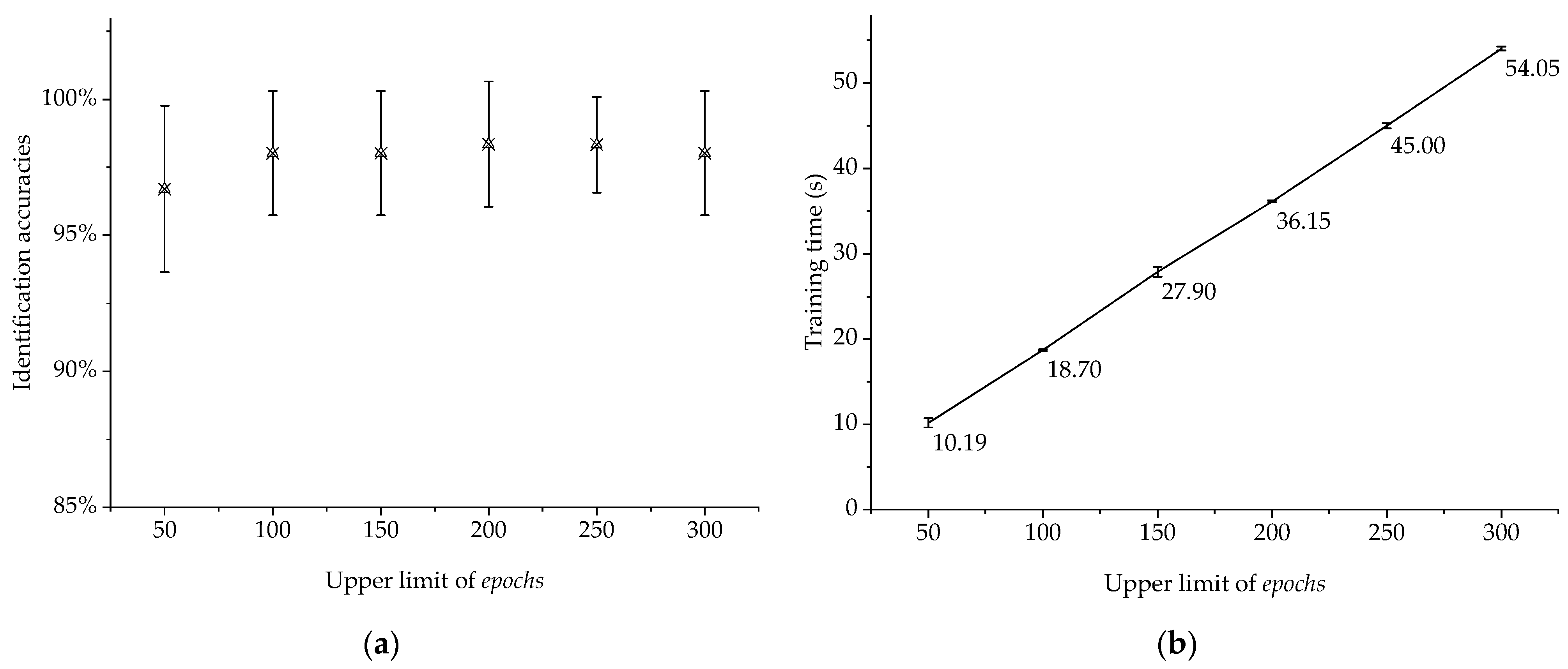
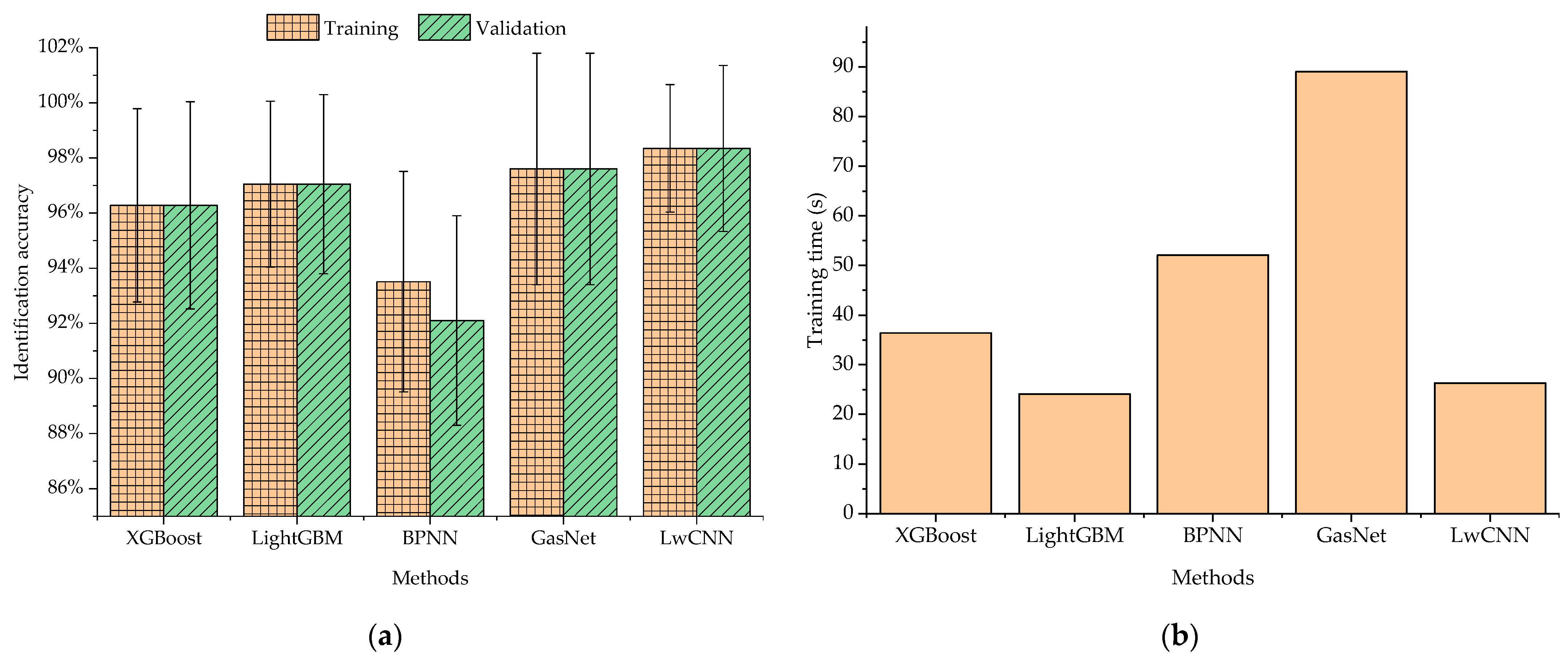
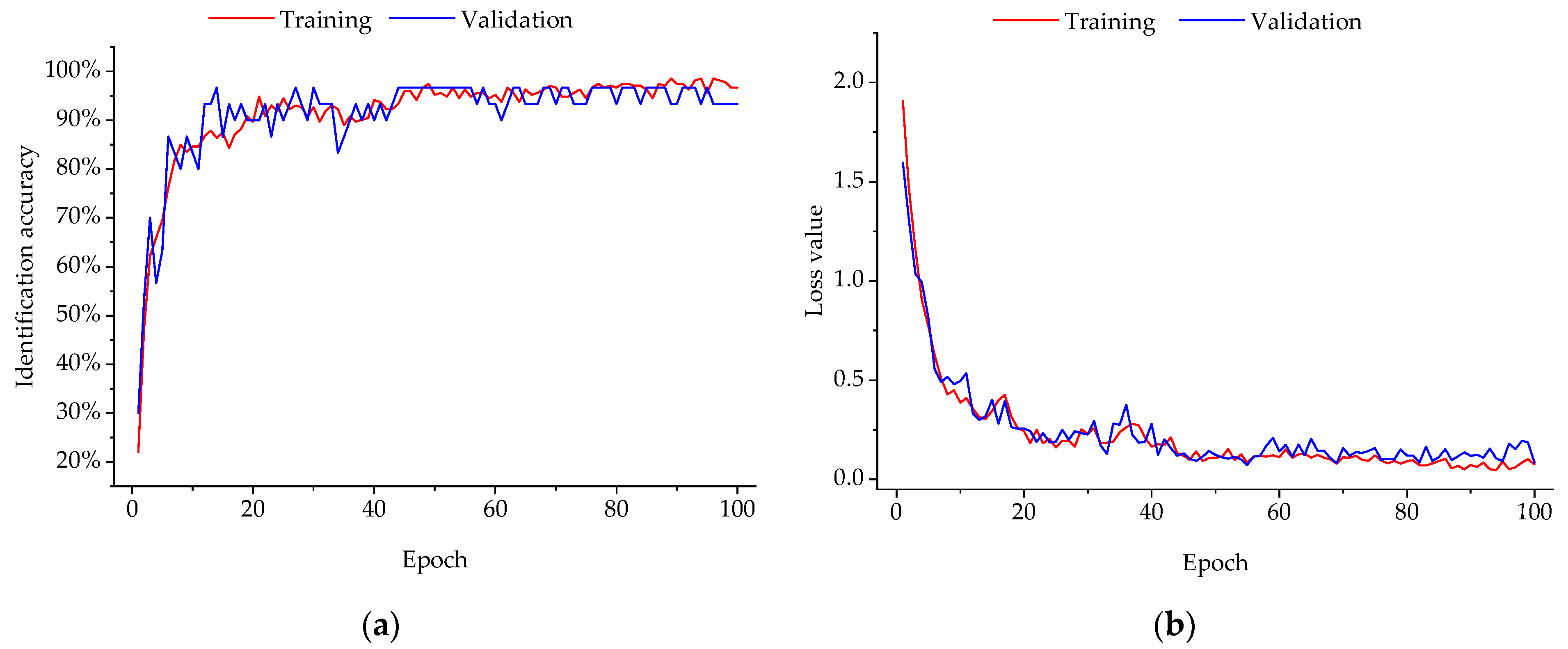
Based on the sampling data, three groups of experiments were conducted. First, the optimal value of maximum training epochs was determined for LwCNN by statistical comparison. Empirically, the number of training epochs can seriously influence the spent training time, which is one of main concerns about using the integrated handheld EN in this paper. Then, a set of orthogonal experiments [31] were conducted to determine the optimal values of the three hyperparameters in LwCNN, which are the convolution kernel number M, the convolution kernel length n, and the dropout proportion λ. Finally, the four benchmark methods, those are, XGBoost, LightGBM, BPNN, and GasNet, were evaluated in 10-fold cross-validation experiments. Based on the experimental results, the performance of LwCNN was compared with the four benchmark methods. As tested in the author’s previous works [3,4], the hyperparameters of XGBoost, LightGBM, BPNN were automatically tunned using the hyperopt Python module [32], which models the parameter tuning process as solving a multi-variant function optimization problem. The time spent for automatic parameter tuning was included in the model training time, since the parameter values are also part of the trained model. For GasNet, the parameter values were fixed as those used in [27].

5. Results and Discussion

5.1. The Measurement Data

As mentioned in Section 4, with respect to each gas sensor, 500 sensing voltage values were sampled in each sampling cycle. The eight sequences of sensing voltage values were concatenated to a 1D vector in the first feature flattening layer of LwCNN. Figure 4 shows the concatenation of the eight sensors’ sensing voltages obtained in a typical sampling cycle. The model names of the eight sensors are TGS2600, TGS2602, TGS2611, TGS2620, MiCS5524, MiCS5914, MiCS6814, and TGS8100.

With respect to each individual gas sensor, each unit of 500 sensing voltages demonstrates a fast rising and relatively slow falling shape. These curve modalities coincide with the characteristics of the used metal oxide semiconductor gas sensors. In Figure 4, different gas sensors obtained different peak values and different rising/falling speeds, while the starting values of different sensors are all equal to zero. Although the absolute gas concentrations in the surrounding space of the eight sensors were the same, different characteristics of the eight sensors caused the different output sensing voltages. The same zero starting values was caused by the baseline subtraction in the preprocessing operation. Because the baseline voltages were subtracted from all the sensing values, the negative impact of the gas residuals on the model training was alleviated for the tested benchmark methods.

5.2. Parameter Tuning

As mentioned in Section 4, the influence of the maximum training epochs on the PI performance of LwCNN was first studied. To focus on the influence of training epochs, the values of M, n, and λ were fixed as 32, 5, and 0.5, respectively. Empirically, it was found that the influence of training epochs on the PI performance did not rely on the values of M, n, and λ. Moreover, the time spent to predict the perfume type with previously trained models are similarly short for all the tested methods. Thus, only the time spent for model training was recorded and compared in this paper. By conducting LwCNN for different epochs, the resulting identification accuracies and training time are shown as error bars in Figure 5a,b, respectively.

As shown in Figure 5a, the identification accuracies generally increased as the upper limit of epochs was changed from 50 to 100. However, when the upper limit of epochs exceeded 100, the identification accuracies did not demonstrate an obvious increasing trend when the upper limit of epochs was increased. This is probably because LwCNN has extracted the utmost information with the current setup of M, n, and λ in about 100 training epochs. According to Figure 5b, the training time demonstrates a positive quasi-linear relationship to the upper limit of epochs. The time spent for training the LwCNN model increased if the model was trained for more epochs, which coincides with the theoretical basis of LwCNN. Thus, the optimal value of training epochs was set as 100 in the following experiments.

To further investigate the influence of M, n, and λ on the PI performance, a set of orthogonal experiments were designed and conducted. In the orthogonal experiments, M, n, and λ were taken as the orthogonal experimental factors. For each experimental factor, four levels were assigned: M, n, and λ were selected from the sets {20, 30, 40, 50}, {3, 5, 7, 9}, and {0.4, 0.5, 0.6, 0.7}, respectively. According to the L₁₆(4³) orthogonal experimental design, 16 value combinations of M, n, and λ were tested. For each of the value combinations, a set of 10-fold cross-validation experiments were conducted.

Table 1. Orthogonal experimental results of utilizing different values for M, n, and λ in LwCNN.

No.	Experimental Factors			Identification Accuracies		Training Time (s)
	M	n	λ	Mean	stdev	Mean	stdev
1	20	3	0.4	97.69%	2.20%	16.31	0.86
2	20	5	0.5	97.37%	2.98%	17.15	0.13
3	20	7	0.6	97.36%	2.06%	17.55	0.16
4	20	9	0.7	97.38%	2.06%	18.25	0.53
5	30	3	0.5	97.37%	2.06%	19.61	0.40
6	30	5	0.6	97.70%	2.20%	20.87	0.24
7	30	7	0.7	97.12%	2.63%	22.04	1.28
8	30	9	0.4	97.69%	2.20%	23.48	0.50
9	40	3	0.6	98.35%	2.31%	26.28	0.39
10	40	5	0.7	97.04%	2.83%	29.46	1.31
11	40	7	0.4	98.02%	2.28%	30.63	1.02
12	40	9	0.5	97.35%	2.59%	31.76	0.51
13	50	3	0.7	97.69%	2.20%	30.24	1.01
14	50	5	0.4	98.02%	2.28%	32.83	0.92
15	50	7	0.5	98.02%	2.28%	34.77	0.63
16	50	9	0.6	97.37%	2.06%	38.57	2.71

lists the means and standard deviations of the corresponding experimental results. For all tested value combinations of M, n, and λ, the mean identification accuracies obtained by LwCNN are higher than 97%. These considerably high identification accuracies verify the feasibility of using LwCNN for solving the EN-based PI problem. The standard deviations of identification accuracies are more or less the same for all the tested value combinations. By setting the value combination of (M, n, λ) as (40, 3, 0.6), LwCNN obtained the highest mean identification accuracy in Table 1. The corresponding median training time, that is, 26.28 s, is acceptable for real EN-based PI applications.

Table 2. The dimensions and trainable parameter numbers of LwCNN when M, n, and λ were set as 40, 3, and 0.6, respectively.

Functional Layers	LwCNN
	Dimensions	Parameters
Input	(4000, 1)	0
Conv1D	(4000, 40)	160
MaxPooling1D	(2000, 40)	0
Conv1D	(2000, 40)	4840
Flattening	(80,000)	0
Fully connected	(6)	480,006
		485,006 (Tot.)

lists the vector dimensions and trainable parameter numbers in the case that the value of (M, n, λ) equals (40, 3, 0.6). The light-weight architecture of CNN accounts for its high time-efficiency in the EN-based PI experiments.

Moreover, the means of training time demonstrate an ascending trend when the number of convolution kernels M increased from 20 to 50. With respect to the same value of M, the mean training time increased when the convolution kernel length n was changed from 3 to 9. Nevertheless, there does not exist obvious relevance between the value of λ and the mean training time can be found. These results can provide important guidance for determining M, n, and λ with the requirement of identification accuracies and training time.

5.3. Comparison Results

To comprehensively evaluate the presented LwCNN method, XGBoost, LightGBM, BPNN, and GasNet were used as the benchmark methods. Figure 6 shows the statistical identification accuracies and training time obtained by LwCNN and the four benchmark methods.

As shown in Figure 6a, LwCNN obtained the highest mean identification accuracy. Even in the case that the values of M, n, and λ were randomly selected from the candidates in Table 1, the corresponding mean identification accuracies obtained by LwCNN are still higher than those obtained by the three benchmark methods. The comparatively higher mean identification accuracy of LwCNN demonstrates the significance of proposing LwCNN for EN-based PI applications. Moreover, LwCNN obtained identical mean identification accuracies for model training and validation. It reveals that LwCNN also can overcome the model overfitting problem, which stagnates the BPNN method.

According to Figure 6b, compared with XGboost, BPNN, and GasNet, LightGBM and LwCNN spent much shorter training time. This phenomenon shows that LwCNN possesses the similar light-weight characteristic as LightGBM. Comparing with XGBoost, the exclusive feature bundling and gradient-based one-side sampling in LightGBM induced its higher time-efficiency. Compared with BPNN, the incorporated convolution, max-pooling, and dropout operations helped LwCNN save a lot of training time and avoid the model overfitting problem. It is noteworthy that LwCNN only spent about a quarter of the time spent by GasNet, which further highlights the significance of presenting LwCNN for quick integrated PI with the computationally constrained ENs. In comparison, the less incorporated operation layers, the front-end feature flattening, and the disposition of 1D convolutional layers in LwCNN mainly account for its obviously higher time-efficiency.

Figure 7 shows the variation of identification accuracies and loss values in a typical trial of training and identification processes. The loss value was defined as the categorical cross entropy, which assesses the distribution differences of identified and actual perfume types. In the first ten epochs, the identification accuracy and loss values exhibited generally fast ascending and descending trends, respectively. Afterwards, the fluctuations of identification accuracy and loss values generally got mild. In both subfigures of Figure 7, the training curve is interwoven with the corresponding validation curve. The similar results obtained in training and validation processes further verify that LwCNN was not influenced by the model overfitting problem.

6. Conclusions

In this paper, a light-weight CNN, namely LwCNN, was presented for identifying the previously unknown perfume type on a self-designed integrated handheld EN, which employs the embedded NVIDIA Jetson nano module as the computing core. Due to the limited computing resource on the EN, LwCNN only utilizes a well-sequenced stack of two feature flattening layers, two 1D convolutional layers, a 1D max-pooling layer, a feature dropout layer, and a fully connected layer. Unlike existing deep CNNs, LwCNN only involves a set of relatively small number of trainable weights. Experimental results demonstrate that LwCNN can significantly improve the time-efficiency of wholly conducting the PI task on the resource-limited NVIDIA Jetson nano module.

A latent condition of the presented experimental results is that the measurement dataset used for training the LwCNN model was successively collected in similar surrounding temperatures and humidity values. If this condition is extremely unsatisfied, the experimental results would deteriorate. Moreover, reducing the volume of training data may also influence the PI performance of LwCNN. The acquisition of the current set of sensing voltage samples were time consuming. Future research works would cover designing more advanced CNN methods with higher robustness and data mining capability.

References

1. Le Roux, A.; Bobrie, F.; Thébault, M. A typology of brand counterfeiting and imitation based on a semiotic approach. J. Bus. Res. 2016, 69, 349–356. [Google Scholar] [CrossRef]
2. Karakaya, D.; Ulucan, O.; Turkan, M. Electronic Nose and Its Applications: A Survey. Int. J. Autom. Comput. 2020, 17, 179–209. [Google Scholar] [CrossRef] [Green Version]
3. Cao, M.; Hu, X. An Integrated Handheld Electronic Nose for Identifying Liquid Volatile Chemicals Using Improved Gradient-Boosting Decision Tree Methods. Electronics 2023, 12, 79. [Google Scholar] [CrossRef]
4. Cao, M.; Ling, X. Quantitative Comparison of Tree Ensemble Learning Methods for Perfume Identification Using a Portable Electronic Nose. Appl. Sci. 2022, 12, 9716. [Google Scholar] [CrossRef]
5. Ayhan, B.; Kwan, C.; Zhou, J.; Kish, L.B.; Benkstein, K.D.; Rogers, P.H.; Semancik, S. Fluctuation enhanced sensing (FES) with a nanostructured, semiconducting metal oxide film for gas detection and classification. Sens. Actuators B Chem. 2013, 188, 651–660. [Google Scholar] [CrossRef]
6. Schmera, G.; Kwan, C.; Ajayan, P.; Vajtai, R.; Kish, L.B. Fluctuation-Enhanced Sensing: Status and Perspectives. IEEE Sens. J. 2008, 8, 714–719. [Google Scholar] [CrossRef]
7. Ju, X.; Lian, F.; Ge, H.; Jiang, Y.; Zhang, Y.; Xu, D. Identification of Rice Varieties and Adulteration Using Gas Chromatography-Ion Mobility Spectrometry. IEEE Access 2021, 9, 18222–18234. [Google Scholar] [CrossRef]
8. Feizi, N.; Hashemi-Nasab, F.S.; Golpelichi, F.; Sabouruh, N.; Parastar, H. Recent trends in application of chemometric methods for GC-MS and GCGC-MS-based metabolomic studies. TrAC Trends Anal. Chem. 2021, 138, 1–13. [Google Scholar] [CrossRef]
9. Li, J.-J.; Song, C.-X.; Hou, C.-J.; Huo, D.-Q.; Shen, C.-H.; Luo, X.-G.; Yang, M.; Fa, H.-B. Development of a Colorimetric Sensor Array for the Discrimination of Chinese Liquors Based on Selected Volatile Markers Determined by GC-MS. J. Agric. Food Chem. 2014, 62, 10422–10430. [Google Scholar] [CrossRef]
10. Jing, Y.; Meng, Q.; Qi, P.; Zeng, M.; Li, W.; Ma, S. Electronic nose with a new feature reduction method and a multi-linear classifier for Chinese liquor classification. Rev. Sci. Instrum. 2014, 85, 1–10. [Google Scholar] [CrossRef]
11. Mei, X.; Wang, B.; Zhe, Z.; Zhao, P.; Hu, X.; Lu, G. Design of electronic nose system for perfume recognition based on support vector machine. J. Jilin Univ. 2014, 32, 355–360. [Google Scholar]
12. Jia, X.; Meng, Q.; Jing, Y.; Qi, P.; Zeng, M.; Ma, S. A New Method Combining KECA-LDA With ELM for Classification of Chinese Liquors Using Electronic Nose. IEEE Sens. J. 2016, 16, 8010–8017. [Google Scholar] [CrossRef]
13. Rehman, A.u.; Bermak, A. Recursive DBPSO for Computationally Efficient Electronic Nose System. IEEE Sens. J. 2018, 18, 320–327. [Google Scholar] [CrossRef]
14. Gewers, F.L.; Ferreira, G.R.; Arruda, H.F.D.; Silva, F.N.; Comin, C.H.; Amancio, D.R.; Costa, L.D.F. Principal Component Analysis: A Natural Approach to Data Exploration. ACM Comput. Surv. 2022, 54, 1–34. [Google Scholar] [CrossRef]
15. Saul, L.K. Think Globally, Fit Locally: Unsupervised Learning of Low Dimensional Manifolds. J. Mach. Learn. Res. 2003, 4, 119–155. [Google Scholar]
16. Globerson, A.; Roweis, S.T. Metric Learning by Collapsing Classes. In Proceedings of the 18th International Conference on Neural Information Processing Systems, Vancouver, BC, Canada, 5–8 December 2005; pp. 451–458. [Google Scholar]
17. Wang, H.; Pi, D.; Sun, Y. On-line support vector machine training algorithm and its application. J. Zhejiang Univ. Eng. Sci. 2004, 38, 1642–1645. [Google Scholar]
18. Sadeghi, B. A BP-neural network predictor model for plastic injection molding process. J. Mater. Processing Technol. 2000, 103, 411–416. [Google Scholar] [CrossRef]
19. Chen, T.; Guestrin, C. XGBoost: A Scalable Tree Boosting System. In Proceedings of the 22nd ACM SIGKDD International Conference on Knowledge Discovery and Data Mining, San Francisco, CA, USA, 13–17 August 2016; pp. 785–794. [Google Scholar]
20. Ke, G.; Meng, Q.; Finley, T.; Wang, T.; Chen, W.; Ma, W.; Ye, Q.; Liu, T.-Y. LightGBM: A highly efficient gradient boosting decision tree. In Proceedings of the 31st International Conference on Neural Information Processing Systems, Long Beach, CA, USA, 4–9 December 2017; pp. 3149–3157. [Google Scholar]
21. Bao, Z.; Xue, R. Survey on deep learning applications in digital image security. Opt. Eng. 2021, 60, 1–32. [Google Scholar] [CrossRef]
22. Lecun, Y.; Bottou, L.; Bengio, Y.; Haffner, P. Gradient-based learning applied to document recognition. Proc. IEEE 1998, 86, 2278–2324. [Google Scholar] [CrossRef] [Green Version]
23. Krizhevsky, A.; Sutskever, I.; Hinton, G. ImageNet Classification with Deep Convolutional Neural Networks. Adv. Neural Inf. Processing Syst. 2012, 25, 84–90. [Google Scholar] [CrossRef] [Green Version]
24. Simonyan, K.; Zisserman, A. Very Deep Convolutional Networks for Large-Scale Image Recognition. In Proceedings of the 3rd International Conference on Learning Representations, San Diego, CA, USA, 7–9 May 2015; pp. 1–14. [Google Scholar]
25. Szegedy, C.; Wei, L.; Yangqing, J.; Sermanet, P.; Reed, S.; Anguelov, D.; Erhan, D.; Vanhoucke, V.; Rabinovich, A. Going deeper with convolutions. In Proceedings of the 2015 IEEE Conference on Computer Vision and Pattern Recognition (CVPR), Boston, MA, USA, 7–12 June 2015; pp. 1–9. [Google Scholar]
26. He, K.; Zhang, X.; Ren, S.; Sun, J. Deep Residual Learning for Image Recognition. In Proceedings of the 2016 IEEE Conference on Computer Vision and Pattern Recognition (CVPR), Las Vegas, NV, USA, 27–30 June 2016; pp. 770–778. [Google Scholar]
27. Peng, P.; Zhao, X.; Pan, X.; Ye, W. Gas Classification Using Deep Convolutional Neural Networks. Sensors 2018, 18, 157. [Google Scholar] [CrossRef] [PubMed] [Green Version]
28. Wang, S.H.; Chou, T.I.; Chiu, S.W.; Tang, K.T. Using a Hybrid Deep Neural Network for Gas Classification. IEEE Sens. J. 2021, 21, 6401–6407. [Google Scholar] [CrossRef]
29. Wang, S.; Yu, X.; Gao, J.; Wang, Z. Age detection of mature vinerger based on electronic tongue and electronic nose combined with DenseNet-ELM. Food Mach. 2022, 38, 72–80. [Google Scholar]
30. Ling, X.W.; Cao, M.L. Perfume identification using a chemical sensor array via LightGBM and prepositive feature reduction. In Proceedings of the 2022 7th International Conference on Intelligent Computing and Signal Processing (ICSP), Xi’an, China, 15–17 April 2022; pp. 1991–1995. [Google Scholar]
31. Box, G.E.P.; Hunter, S.; Hunter, W.G. Statistics for Experiments: Design, Innovation and Discovery, 2nd ed.; Wiley: Hoboken, NJ, USA, 2005. [Google Scholar]
32. Bergstra, J.; Yamins, D.; Cox, D.D. Making a Science of Model Search: Hyperparameter Optimization in Hundreds of Dimensions for Vision Architectures. In Proceedings of the 30th International Conference on Machine Learning, Atlanta, GA, USA, 16–21 June 2013; pp. 115–124. [Google Scholar]
Figure 1. Architecture of the SMUENOSEv2 [3]. The components outside and inside the dashed round rectangle are gas route and electronic components, respectively. The red bold numbers 1 and 2 stand for two sub-routes at the downflow side of the three-way valve.
Electronics 12 01041 g001
Figure 2. Flow-chart of the LwCNN operation architecture in a single training epoch.
Electronics 12 01041 g002
Figure 3. Illustration of the operations in different layers of the LwCNN. For clarification, duplicated layers and the activation layers are not included.
Electronics 12 01041 g003
Figure 4. The flattened 1D vector yielded by concatenating the preprocessed measurements of the eight gas sensors in SMUENOSEv2.
Electronics 12 01041 g004
Figure 5. The error bars of the results obtained by training the LwCNN model for different numbers of epochs: (a) Error bars of the identification accuracies; (b) Error bars of the time spent for training a single LwCNN model.
Electronics 12 01041 g005
Figure 6. The statistical results obtained by XGBoost, LightGBM, BPNN, GasNet, and LwCNN with the same sampling dataset: (a) The mean and standard deviation of identification accuracies; (b) The mean and standard deviation of time spent for model training.
Electronics 12 01041 g006
Figure 7. The identification accuracies and loss values at different epochs in a typical trial of training and identification processes: (a) the variation of identification accuracy in a typical trial; (b) the variation of loss value in a typical trial.
Electronics 12 01041 g007