DOA Estimation Based on Convolutional Autoencoder in the Presence of Array Imperfections

Abstract

Array imperfections may exist in an antenna system subject to non-ideal design and practical limitations. It is difficult to accurately model array imperfections, and thus complicated algorithms are usually inevitable for model-based methods to estimate the direction of arrival (DOA) with imperfect arrays. Deep neural network (DNN)-based methods do not need to rely on pre-modeled antenna array geometries, and have been explored to handle flawed array models because of their better flexibility than model-based methods. The DNN autoencoder (DAE) method has been proposed for the array imperfection problem, which decomposes the input into multiple components in different spatial subregions. These components have more concentrated distributions than the original input, which avoid a large number of connections and nodes used in the layers to realize DOA estimation classifiers. In this paper, we study the convolutional AE (CAE) method that substantially focuses on the learning of local features in a different manner from the previous DAE method. The advantage of the convolutional operation using a kernel in CAE is to capture features in a more efficient manner than the DAE, and thus be able to reduce the number of parameters that are required to be trained in the neural networks. From the numerical evaluation of DOA estimation accuracy, the proposed CAE method is also more resistant to the noise effect than the DAE method such that the CAE method has better accuracy at a lower signal-to-noise ratio.

1. Introduction

Antenna arrays have been widely used for finding signal sources and concentrating beam energy in addition to suppress communication interferences. For example, the direction of arrival (DOA) estimation with the use of antenna arrays has revealed a diverse range of applications such as wireless communications, radar, and sonar, etc. The most classic DOA estimation algorithms are subspace-based methods, e.g., the multiple signal classification (MUSIC) algorithm [1], estimation of signal parameters via rotational invariance techniques (ESPRIT) algorithm [2], etc., and their extended variants [3,4,5,6]. These methods are developed based on the angle mapping relationship between the signal direction and the antenna array, assumed that the relationship between a mapping and the incident angle is reversible. Based on this assumption, the array output can be matched by the mapping to achieve directional estimation. The DOA estimation performance of these parametric estimation methods depends largely on the mathematical model between the mapping and the incident angle, the mapping from the direction of the signal source to the antenna array output, and the inverse mapping from the antenna output to the direction of the signal source.

Due to non-ideal antenna design, limitations of practical implementation, and mutual interferences between antennas, there may be various imperfections existing in array systems [7,8,9]. In a real system, the mapping between the signal direction and the antenna array output is much more complicated than the mathematical model that is usually expressed in the literature [10]. There are various drawbacks in array systems because they are not easy to be accurately modeled such that incorrect models can also cause a significant performance degradation on DOA estimation. In order to reduce the impact of various imperfections, the past works, as found in the literature, merely established simplified models to describe the effect of array imperfections. Most of the problems with simplified array imperfections in mathematical models often consider the following factors: antenna position error, antenna gain and phase error, and mutual interference between antennas, etc. [11]. However, these simplifications and assumptions of parameters and models may still deviate from the actual antenna situation to some degree. In addition, there may be a combination of imperfections in the actual system, which is more difficult to accurately model and calibrate [12] because developing parametric methods to solve these problems is quite difficult. Therefore, it is difficult to find new parametric methods in this research area.

Recent research works have introduced machine learning and deep learning techniques for DOA estimation problems [13,14,15,16,17]. Since machine learning and deep learning methods are data-driven, they do not rely on the mapping between signal direction and antenna arrays as well as their modeling and assumptions about various array imperfection patterns. In the literature, machine learning methods have been proposed to be better than subspace-based methods in computational complexity [13], and have comparable performance with them in experiments [14]. However, machine learning techniques demonstrate a satisfying performance in the case when the training and test data have nearly identical distributions. In a practical application of considering many unknown parameters for an imperfect array, it is difficult to reach such an ideal condition with enough training data set to cover the distributions of all test data as noted in [9]. The autocalibration method is another appealing approach widely studied to deal with imperfect arrays for DOA estimation [18,19,20]. Most autocalibration methods still rely on accurate mathematical modeling for imperfect arrays and, besides, the combined effects of multiple kinds of imperfections probably exist in practical systems. Those practical limitations make the problem difficult to be modeled precisely for perfect calibration. In the past few years, some literature has introduced the use of deep learning techniques to solve the DOA estimation and localization problem for microphone arrays when considering very serious environments such as dynamic acoustic signals [15], reverberation environments [16], and broadband signals. In such applications, it is difficult to model the propagation of the signal to be analyzed, and it is also rather difficult to solve these problems using parametric methods. However, deep learning methods can reconstruct complex propagation models based on training data, and then estimate the direction and location of sound sources. This approach first converts the original sound signal into the time–frequency domain, and then takes the converted signal as the input of the deep neural network (DNN) [17]. DOA estimation of sound signals can be implemented in a similar way to pattern recognition of images.

The use of autoencoders (AE) to handle wireless positioning was mentioned in [21,22,23,24]. Ref. [21] designs a sparse AE network to automatically learn discriminative features from the wireless signals and merges the learned features into a softmax-regression-based machine learning framework to simultaneously realize location, activity, and gesture recognition. Ref. [22] proposes a convolutional AE (CAE) for the device-free localization problem. Different from the fully connected layers in an AE, a CAE consists of a convolutional encoder and the corresponding deconvolutional decoder. The encoder part is implemented to extract feature maps from input images, while the decoder part is used to reconstruct information from the learned feature maps. In [9,25], the framework based on the DNN AE (DAE) technique is proposed for DOA estimation concerning array imperfections. Ref. [9] first calculates the cross space matrix (CSM) of the array output, uses it as the input of the DAE, and then introduces the multitasking AE before multilayer classifiers to decompose the input signal vector into several spatial subregions. A series of parallel multilayer classifiers was finally introduced to implement DOA estimation. It features a multitasking AE executing an operation similar to a spatial filter to preprocess signal samples, which helps to narrow the spatial range covered by DOA estimates for input samples, thereby greatly enhancing the versatility of the proposed method in unknown situations. If a set of training samples is used to train a DAE, the corresponding DOA estimation method does not need to be processed with any prior assumptions about them.

For DOA estimation with DNN [26,27], a key point is how to extract important features that represent different locations. In this paper, we integrate a convolutional neural network with AE to build a new CAE structure to deal with DOA estimation problems. To explain the innovation in the new method, we state the following.

(1)

The new structure combines the advantages of convolutional kernels and DAE, in which the convolutional kernel is better suitable for learning local features in different subregions and a hierarchical framework similar to a DAE remains to deal with DOA estimation.

(2)

A fully connected neural network is used in a DAE, where every neuron between two adjacent layers is connected. When the feature dimension of the input layer becomes very high, the parameters that a fully connected network needs to train will increase dramatically, leading to the calculation speed becoming slower. In the proposed CAE, the neurons of the convolutional layer are only connected to some neuron nodes in the previous layer.

(3)

The connections between neurons are not fully connected, and the weight and offset of the connections between some neurons in the same layer are shared, which greatly reduces the number of parameters that need to be trained.

(4)

The convolutional operation in CAE is essentially an input-to-output mapping with DNN, which can learn a large number of mapping relationships between input and output, without the need for any precise mathematical expression between input and output.

The remainder of this paper is organized as follows. Section 2 describes a simplified model about the imperfections in a non-ideal array antenna. Section 3 gives a brief review on the DAE structure while Section 4 explains the proposed CAE structure. Section 5 demonstrates the numerical results, and Section 6 summarizes our work.

2. Signal Model with Array Imperfections

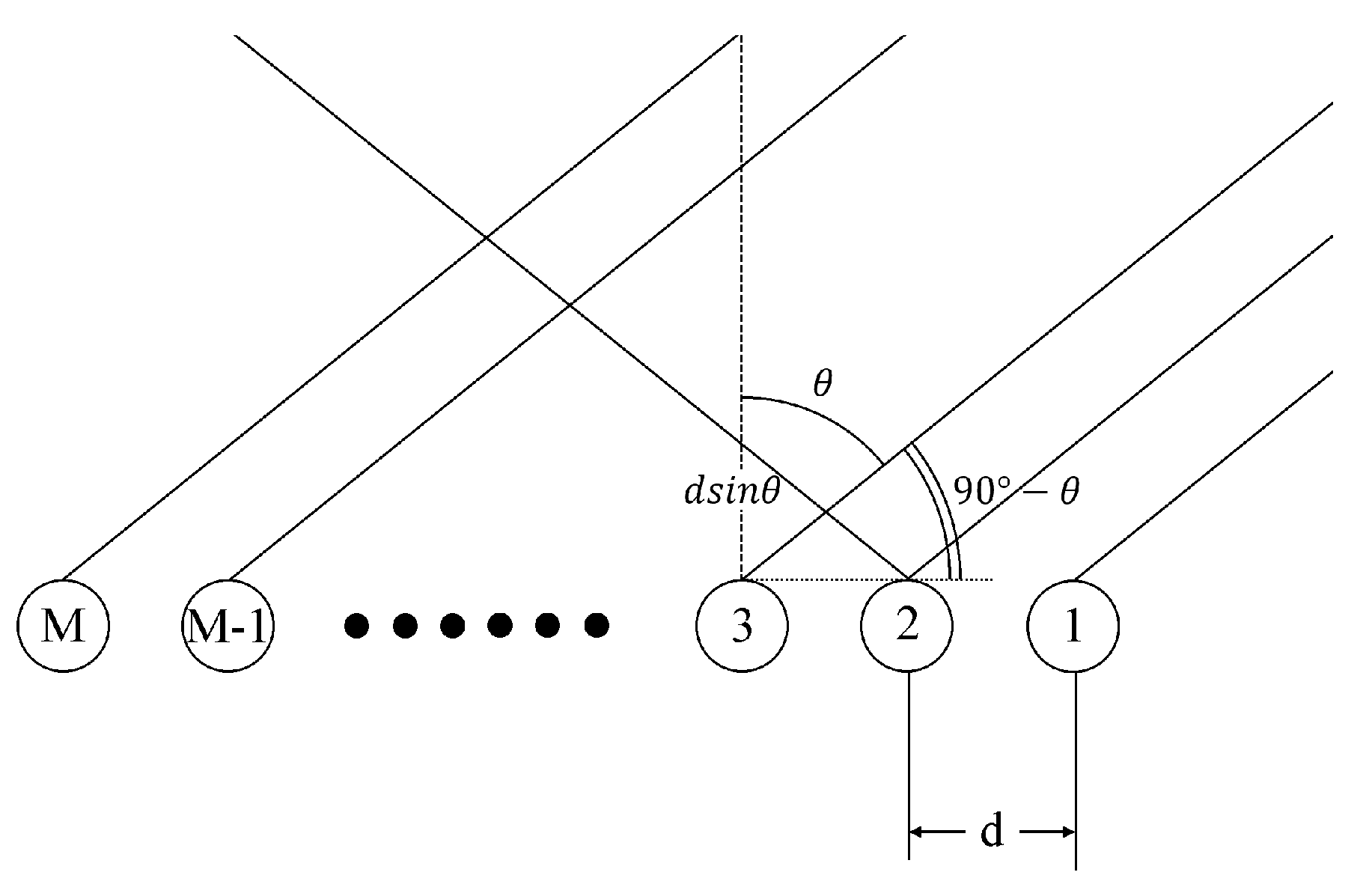
Consider that a planar uniform linear array (ULA) consists of M antenna elements, and d represents the distance between two neighboring elements of the receiving array. Assume that the signal source is far-field and the signal $s\left(t\right)$ impinges on the antenna elements in straight lines. The azimuth of the incident signal is given by $\theta$, as shown in Figure 1. Let ${\tau }_m$ denote the propagation delay of the mth antenna element, then ${\tau }_m=(m-1)dsin\theta /c$, $m=1,2,\cdots ,M$, and c is the speed of light. The wave path difference due to the time delay ${\tau }_m$ will cause a phase shift such that the signal received by the mth antenna at time $t_n$ can be written as

$$x_m\left(t_n\right)=s\left(t_n\right)e^{-j\frac{2\pi }{\lambda }(m-1)dsin\theta },$$

(1)

where $\lambda$ is the wavelength of the signal. From (1), the $M\times 1$ signal vector $\mathbf{x}\left(t_n\right)={[x_1\left(t_n\right)x_2\left(t_n\right)\cdots x_M\left(t_n\right)]}^T$ received by M antennas can be expressed as

$$\mathbf{x}\left(t_n\right)=\mathbf{a}\left(\theta \right)s\left(t_n\right),$$

(2)

where ${[·]}^T$ denotes the transpose of a vector and $\mathbf{a}\left(\theta \right)={[1e^{-j\frac{2\pi }{\lambda }dsin\theta }\cdots e^{-j\frac{2\pi }{\lambda }(M-1)dsin\theta }]}^T$ is the steering vector. Suppose $\mathbf{v}\left(t_n\right)=[v_1\left(t_n\right)$$v_2\left(t_n\right)$⋯$v_M\left(t_n\right){]}^T$ is the additive zero-mean white Gaussian noise (AWGN) vector with covariance matrix ${\sigma }^2\mathbf{I}$, and the received signal vector with M antennas can be rewritten as

$$\mathbf{x}\left(t_n\right)=\mathbf{a}\left(\theta \right)s\left(t_n\right)+\mathbf{v}\left(t_n\right).$$

(3)

Three typical kinds of array imperfections are considered in our framework, including gain and phase inconsistence, antenna position error, and inter-antenna mutual coupling. Those imperfections cause different deviations to the steering vector in (2). Denote the collection of imperfection parameters by $\mathbf{e}$ and the ideal steering vector by $\mathbf{a}\left(\theta \right)$. We represent the array responding function due to imperfections as $\mathbf{a}(\theta ,\mathbf{e})$. In practice, array imperfections are complicated to be formulated with concise mathematical models, and we consider a simplified model in this paper as $\mathbf{a}(\theta ,\mathbf{e})$.

Let $\mathbf{e}=\{{\mathbf{e}}_{gain},{\mathbf{e}}_{phase},{\mathbf{e}}_{pos},{\mathbf{E}}_{mc}\}$ denote the collection of array imperfections, in which those elements represent for the imperfections of gain and phase biases, position error, and the mutual coupling matrix, respectively. From [9], the perturbed array responding function can be written as

$$\begin{array}{cc}\hfill \mathbf{a}(\theta ,\mathbf{e})=& ({\mathbf{I}}_M+{\delta }_{mc}\rho {\mathbf{E}}_{mc})\times ({\mathbf{I}}_M+\mathrm{diag}\left({\delta }_{gain}\rho {\mathbf{e}}_{gain}\right))\hfill \\ & \times \mathrm{diag}\left(e^{j{\delta }_{phase}\rho {\mathbf{e}}_{phase}}\right)\times \mathbf{a}(\theta ,{\delta }_{pos}\rho {\mathbf{e}}_{pos}),\hfill \end{array}$$

(4)

where ${\delta }_{mc},{\delta }_{gain},{\delta }_{phase},$ and ${\delta }_{pos}\in \{0,1\}$ are used to indicate whether a certain kind of imperfection exists, $\rho \in [0,1]$ is used to specialize the strength of the imperfection, ${\mathbf{I}}_M$ is the $M\times M$ identity matrix, and $\mathrm{diag}(·)$ denotes the diagonal matrix of the given vector in $(·)$.

Let ${\mathbf{e}}_{mc}$ denote the inter-channel mutual coupling coefficient vector, then

$$\begin{array}{cc}\hfill {\mathbf{e}}_{mc}=& {\left[0{\gamma }_{mc}^1\cdots {\gamma }_{mc}^{M-1}\right]}^T,\hfill \end{array}$$

(5)

where the elements in ${\mathbf{e}}_{mc}$ contain the power terms of the coupling coefficient ${\gamma }_{mc}$, where ${\gamma }_{mc}=\alpha e^{j\beta }$, $\alpha \in [0,1]$ and $\beta \in [-\pi ,\pi ]$. Then, ${\mathbf{E}}_{mc}$ is a Toeplitz matrix with the vector ${\mathbf{e}}_{mc}$, that is [28],

$$\begin{array}{cc}\hfill {\mathbf{E}}_{mc}& =\mathrm{Toeplitz}\left({\mathbf{e}}_{mc}\right)\hfill \\ & =\left[\begin{array}{cccccc}0& {\gamma }_{mc}^1& {\gamma }_{mc}^2& \cdots & \cdots & {\gamma }_{mc}^{M-1}\\ {\gamma }_{mc}^1& 0& {\gamma }_{mc}^1& \ddots & & ⋮\\ {\gamma }_{mc}^2& {\gamma }_{mc}^1& \ddots & \ddots & \ddots & ⋮\\ ⋮& \ddots & \ddots & \ddots & {\gamma }_{mc}^1& {\gamma }_{mc}^2\\ ⋮& & \ddots & {\gamma }_{mc}^1& 0& {\gamma }_{mc}^1\\ {\gamma }_{mc}^{M-1}& \cdots & \cdots & {\gamma }_{mc}^2& {\gamma }_{mc}^1& 0\end{array}\right].\hfill \end{array}$$

(6)

${\mathbf{e}}_{gain}$ in (4) represents for the gain bias of M antennas [29]

$$\begin{array}{cc}\hfill {\mathbf{e}}_{gain}=& {\left[0{\gamma }_{gain}^{\left(1\right)}\cdots {\gamma }_{gain}^{(M-1)}\right]}^T,\hfill \end{array}$$

(7)

where ${\gamma }_{gain}^{\left(m\right)}\in [0,1]$. ${\mathbf{e}}_{phase}$ in (4) represents for the phase bias of M antennas

$$\begin{array}{cc}\hfill {\mathbf{e}}_{phase}=& {\left[0{\gamma }_{phase}^{\left(1\right)}\cdots {\gamma }_{phase}^{(M-1)}\right]}^T,\hfill \end{array}$$

(8)

where ${\gamma }_{phase}^{\left(m\right)}\in [-\pi ,\pi ]$. ${\mathbf{e}}_{pos}$ in (4) represents for the position bias of M antennas

$$\begin{array}{cc}\hfill {\mathbf{e}}_{pos}=& {\left[0{\gamma }_{pos}^{\left(1\right)}\cdots {\gamma }_{pos}^{(M-1)}\right]}^T\times d,\hfill \end{array}$$

(9)

where ${\gamma }_{pos}^{\left(m\right)}\in [0,1]$. When the positions of M antennas are skewed, the steering responding function $\mathbf{a}(\theta ,\rho {\mathbf{e}}_{pos})$ becomes

$$\begin{array}{c}\hfill \mathbf{a}(\theta ,\rho {\mathbf{e}}_{pos})={\left[\begin{array}{cccc}0& e^{-j\frac{2\pi }{\lambda }(1+\rho {\gamma }_{pos}^{\left(1\right)})dsin\theta }& \cdots & e^{-j\frac{2\pi }{\lambda }(M-1+\rho {\gamma }_{pos}^{(M-1)})dsin\theta }\end{array}\right]}^T.\end{array}$$

(10)

In the literature, there are mainly four possible approaches to deal with the imperfection problem: model-based algorithms, machine learning methods, such as support vector regression (SVR) mentioned in [9], autocalibration, and deep learning methods. Those four approaches have their individually better application scenarios and situations. For example, model-based and autocalibration methods rely on the mathematical model of imperfections to find solutions. With a precise model, they can reach a good theoretical RMSE performance. The machine learning methods usually lack robustness to noisy training data sets. However, without the assumption of knowing precise imperfection model as a priori knowledge, machine learning and deep learning algorithms have been recently considered to estimate the angle between the incident signal and the array antennas, which seems more flexible than other approaches and general subspace-based estimation algorithms, such as MUSIC, ESPRIT, etc., to yield robust DOA estimation for imperfect arrays in practical environments.

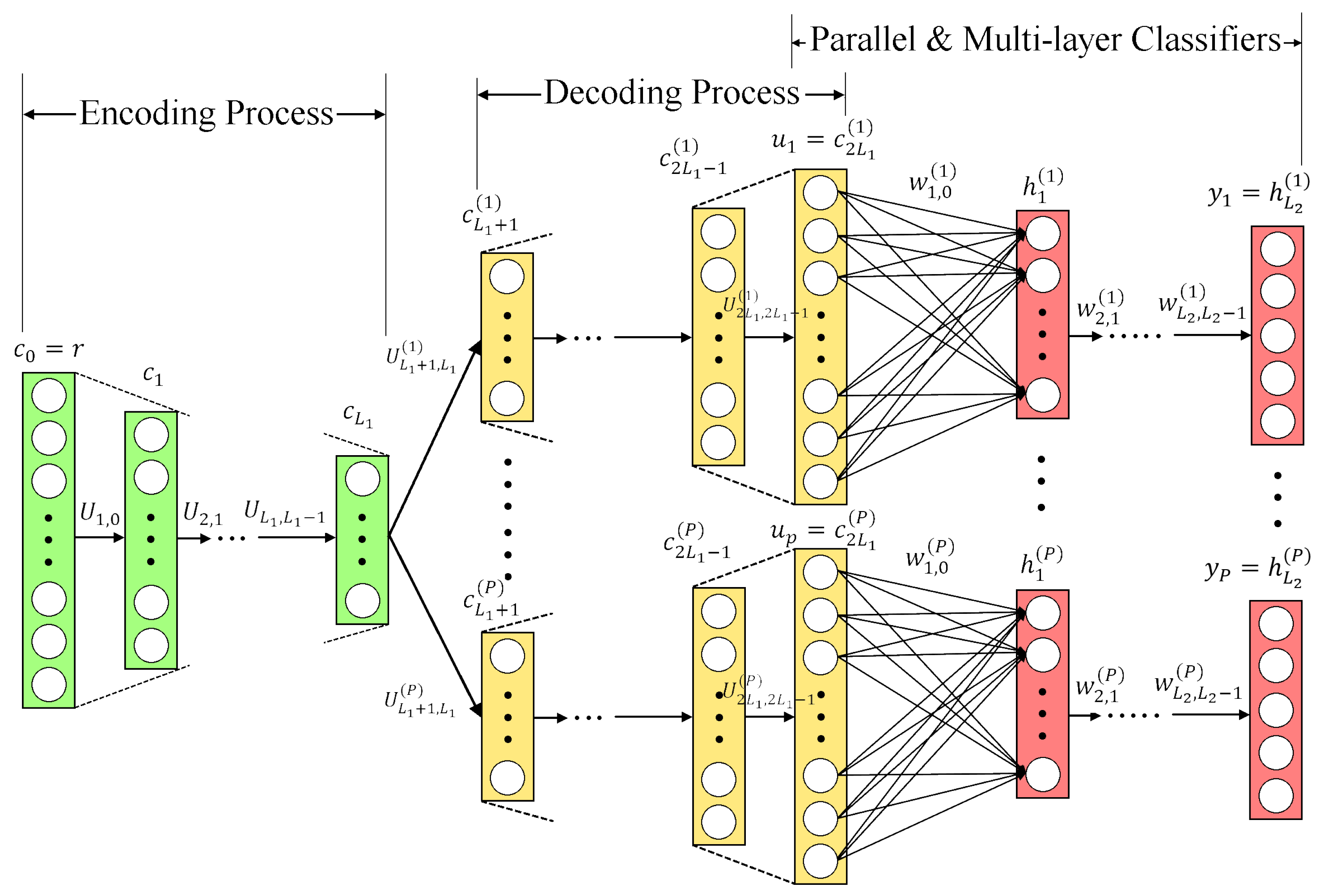
3. DOA Estimation with DNN Autoencoder

The DAE method uses parallel multilayer classifiers and performs as a spatial filter to divide the full input DOA range into multiple subregions, helping to reduce the computational burden required in the classifiers. There are two main parts in a DAE: the front-end is the multitasking AE behaving as a spatial filter, and then parallel multilayer classifiers are connected at the back-end to estimate the DOA of the incident signal. In [9], the multitasking AE is designed to decompose the incident signal into P spatial subregions, and when the input signal is located in the pth subregion, the output of the pth decoder is used as the input of the pth multilayer classifier. If the input DOA does not belong to the pth subregion, the pth decoder output equals to $\mathbf{0}$. The main advantage is that in a multitasking AE, each decoder output covers a narrower spatial subregions, making the incident signal distribution more concentrated. This allows subsequent parallel multilayer classifiers to learn the DOA features located in corresponding subregions, and therefore makes training easier.

3.1. Data Preprocessing for DAE

Consider that the signal received by the antenna array is contaminated by AWGN, where all noise $v_m\left(t_n\right)$ are not related to the source signal $s\left(t_n\right)$. However, with the M antennas and over a period of time for the received signal vector $\mathbf{x}\left(t_n\right)$, antenna’s imperfections can be found through the statistical characteristics related to each other. We collect the received signal of N snapshots and calculate the CSM of the signals as [30]

$$\mathbf{R}=\frac{1}{N}\sum _{n=1}^N\mathbf{x}\left(t_n\right){\mathbf{x}}^H\left(t_n\right).$$

(11)

Reformulate all the elements of the matrix $\mathbf{R}$ as a vector $\overline{\mathbf{r}}$

$$\begin{array}{ccc}\hfill \overline{\mathbf{r}}& =& \left\{{\mathbf{R}}_{m_1,m_2}\right\}\in C^{M^2\times 1}\hfill \end{array}$$

(12)

$$\begin{array}{ccc}\hfill \mathbf{r}& =& {\left[\mathrm{Re}\left\{\overline{\mathbf{r}}\right\}\mathrm{Im}\left\{\overline{\mathbf{r}}\right\}\right]}^T/∥\overline{\mathbf{r}}∥\hfill \end{array}$$

(13)

where ${\mathbf{R}}_{m_1,m_2}$ represents the $(m_1,m_2)$th element in matrix $\mathbf{R}$, $\mathrm{Re}(·)$ and $\mathrm{Im}(·)$ take the values from the real part and the imaginary part, respectively, and finally we rearrange the vector $\mathbf{r}$ as the input for AE.

The data length for preprocessing of the AE can vary depending on the selected collection of ${\mathbf{R}}_{m_1,m_2}$. All elements of the CSM can be used as the input vector, in which case $m_1,m_2=1,2,\cdots ,M$. In order to reduce the size of the input vector to the AE, only some elements in CSM can be taken as the input vector. For example, in [22], the elements of the diagonal matrix are excluded to reduce the noise effect, and considering the conjugate symmetry of the CSM, the elements of the lower left triangular matrix are discarded. Only the elements of the upper right triangular matrix are selected as the input vector to the AE. In this case, $m_1=1,2,\cdots ,M-1$, while $m_2=m_1+1,m_1+2,\cdots ,M$. It is worth noting that N should be large enough to reduce the influence of noise on off-diagonal upper right or lower left matrix elements in order to calculate the CSM for better results.

3.2. Encoding and Decoding for DAE

As depicted in Figure 2, the encoder of AE compresses the dimension of the input vector for a lower one to extract the main components in the original input, and then goes through the decoding process to recover the original dimension, in which the input vector will be decoded and restored in the subregion to which it belongs. The encoding–decoding process is efficient to reduce the influence of noise and input perturbations.

First, assume that each of the encoder and decoder has $L_1$ layers, and the vector $\mathbf{c}$ has the same dimension in the $(L_1-l_1)$th and the $(L_1+l_1)$th layers for $0<l_1\le L_1$. Additionally, notice that the dimension of ${\mathbf{c}}_{l_1}^{\left(p\right)}$ is smaller than that of ${\mathbf{c}}_{l_1-1}^{\left(p\right)}$. The adjacent layers of the AE are fully connected using a feedforward neural network structure, expressed as

$$\begin{array}{cc}\hfill {\mathbf{net}}_{l_1}^{\left(p\right)}& ={\mathbf{U}}_{l_1,l_1-1}^{\left(p\right)}{\mathbf{c}}_{l_1-1}^{\left(p\right)}+{\mathbf{b}}_{l_1}^{\left(p\right)}\hfill \\ \hfill p=& \left\{\begin{array}{c}\begin{array}{c}1\mathtt{for}{l}_1=1,2,\cdots ,L_1\hfill \\ 1,2,\cdots ,P\mathtt{for}{l}_1=L_1+1,\cdots ,2L_1\hfill \end{array}\end{array}\right.\hfill \\ \hfill {\mathbf{c}}_{l_1}^{\left(p\right)}=& f\left[{\mathbf{net}}_{l_1}^{\left(p\right)}\right],\hfill \end{array}$$

(14)

where superscript ${(·)}^{\left(p\right)}$ is associated with the pth subregion, subscripts ${(·)}_{l_1}$ and ${(·)}_{l_1-1}$ denote the layer indices, ${\mathbf{c}}_{l_1}^{\left(p\right)}$ is the $l_1$th layer output of the pth AE, ${\mathbf{c}}_0=\mathbf{r}$ represents for the initial input vector of the AE, ${\mathbf{U}}_{l_1,l_1-1}^{\left(p\right)}$ is the weight matrix from the $(l_1-1)$th to the $l_1$th layer for the pth subregion, ${\mathbf{b}}_{l_1}^{\left(p\right)}$ is the additive bias in the $l_1$ layer, and $f[·]$ denotes the activation function in the $l_1$ layer, which can be the Relu function, that is,

$$f\left(\alpha \right)=max(0,\alpha ).$$

(15)

The multitasking AE intends to decompose the input into P spatial subregions. A simple partition method is to choose $P+1$ directions ${\theta }^{\left(0\right)}<{\theta }^{\left(1\right)}<\cdots <{\theta }^{\left(P\right)}$, satisfying ${\theta }^{\left(1\right)}-{\theta }^{\left(0\right)}={\theta }^{\left(2\right)}-{\theta }^{\left(1\right)}=\cdots ={\theta }^{\left(P\right)}-{\theta }^{(P-1)}$ and $[{\theta }^{\left(0\right)},{\theta }^{\left(P\right)})$ is the full spatial range covered by the incident signal. If a signal impinging from the pth subregion is used as the input to the AE, the pth decoder output ${\mathbf{c}}_{2L_1}^{\left(p\right)}$ equals to the input $\mathbf{r}$ while other decoder outputs equal zero.

3.3. DAE Multilayer Classifiers

Each of the P groups of parallel multilayer classifiers takes the output of its decoder as input, and then a set of fully connected multilayer neural networks are used to estimate the spatial spectrum for the corresponding subregions individually. The output of each AE ${\mathbf{u}}_p$ is only located in a smaller spatial range than the full range. Since the antenna array has a similar steering responding function in adjacent space, the output of the AE ${\mathbf{u}}_p$ is more centrally distributed than the original input signal $\mathbf{r}$, and the adjacent layers of parallel multilayer classifiers are connected using feedforward neural networks as

$$\begin{array}{cc}\hfill {\mathbf{net}}_{l_2}^{\left(p\right)}& ={\mathbf{W}}_{l_2,l_2-1}^{\left(p\right)}{\mathbf{h}}_{l_2-1}^{\left(p\right)}+{\mathbf{q}}_{l_2}^{\left(p\right)}\hfill \\ \hfill & \mathtt{for}p=1,2,\cdots ,P,l_2=1,2,\cdots ,L_2\hfill \\ \hfill {\mathbf{h}}_{l_2}^{\left(p\right)}=& f\left[{\mathbf{net}}_{l_2}^{\left(p\right)}\right],\hfill \end{array}$$

(16)

where ${\mathbf{h}}_{l_2}^{\left(p\right)}$ is the output vector in the $l_2$th layer of the pth classifier, ${\mathbf{W}}_{l_2,l_2-1}^{\left(p\right)}$ is the weight matrix between the $(l_2-1)$th and the $l_2$th layer of the p subregion, ${\mathbf{q}}_{l_2}^{\left(p\right)}$ is the additive bias vector in the $l_2$th layer of the pth subregion, and $f[·]$ is the activation function in the $l_2$th layer. Denote ${\mathbf{y}}_p={\mathbf{h}}_{L2}^{\left(p\right)}$ as the output of the last layer. After obtaining all the outputs of the P parallel classifiers, the P outputs are combined in order as a vector

$$\mathbf{y}={[{\mathbf{y}}_1^T{\mathbf{y}}_2^T\cdots {\mathbf{y}}_P^T]}^T$$

(17)

to estimate the spatial spectrum with the input $\mathbf{r}$. To achieve DOA estimation based on the spectrum estimate, the nodes close to the true signal direction in the output $\mathbf{y}$ have positive values, while other node outputs equal zero.

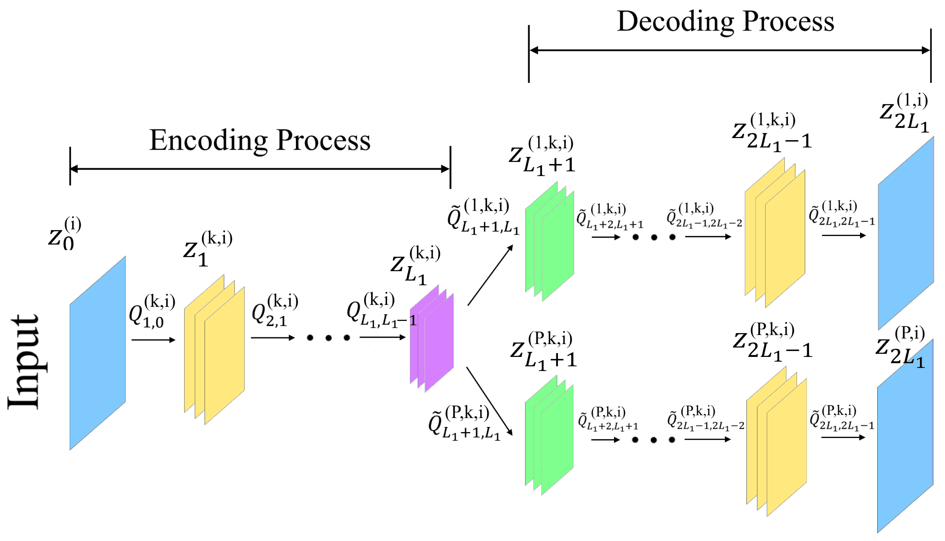
4. Convolutional Autoencoder for DOA Estimation

The CAE structure integrates the advantages of convolutional neural networks (CNNs) and AE. Before elaborating the CAE method for DOA estimation, three points about CAE can be stated as follows.

Motivation. The main feature of CAE differing from DAE [9] is to introduce convolutional kernels used in CNN to the AE structure. CNN is known for its excellent 2D image processing capabilities, which learns extracted features in a nonlinear manner based on convolutional and pooling layers in specific regions of the input feature maps, and is paired with a few fully connected layers for the output. CNN does not only reduce computational costs, but also improves feature extraction capabilities. The encoder part of AE learns the low-dimensional representation characteristics of the input data, called the code layer, and the decoder part reconstructs the code layer back to the original dimension. It is worth noting that under the structure of an AE, the input data are processed in a vector form, and the layers are fully connected. CAE consists of a convolutional encoder and the corresponding deconvolution decoder, which extracts feature maps from the input matrix in the encoder part while reconstructing information from feature maps in the decoder.

Structure. The proposed CAE structure is plotted in Figure 3. Assume that the full DOA range is decomposed into P subregions in the decoding process. In addition to data preprocessing, a CAE is divided into two parts: a multitasking AE for spatial filters, and a set of parallel multilayer classifiers for DOA estimation. For data preprocessing in CAE, the real and imaginary parts of the CSM are separated as two individual input channels. The multitasking AE is conceptually similar to that used in DAE. The inputs are first compressed through the encoding process, and then the feature maps are recovered through the decoding process. The training process learns from the difference between the output of the decoder and the original input to obtain the CAE parameters.

Innovation. The CAE adds each node of the AE to a kernel to perform convolutional operation. The main purpose of the convolutional operation is to capture features, where some regional features of the input channel are selected by the kernel to produce all feature maps. Hence, CAE can capture features in a more efficient manner than DAE and reduce the number of parameters that are required to be trained in the neural networks.

4.1. Data Preprocessing for CAE

Imagine that when CAE is applied to image processing, a color image is used as a matrix input such as a size of $320\times 320$ color image containing three channels, R, G, and B, regarded as matrices of $320\times 320\times 3$. Here we take a similar approach, decomposing the real and imaginary parts of the CSM in (11) as the input matrices of two independent channels

$$\begin{array}{ccc}\hfill {\mathbf{z}}_0^{\left(1\right)}& =& \mathrm{Re}\left\{\mathbf{R}\right\},\hfill \end{array}$$

(18)

$$\begin{array}{ccc}\hfill {\mathbf{z}}_0^{\left(2\right)}& =& \mathrm{Im}\left\{\mathbf{R}\right\},\hfill \end{array}$$

(19)

where ${\mathbf{z}}_0^{\left(1\right)}$ and ${\mathbf{z}}_0^{\left(2\right)}$ represent the two channel input matrices to CAE.

4.2. Encoding and Decoding for CAE

The structure of CAE is intuitively similar to that of AE, except for the convolutional operation. Assuming that each layer operates the convolution with K kernels, K feature maps can be produced correspondingly. The representation of the kth feature map during encoding is

$$\begin{array}{cc}\hfill {\mathbf{cov}}_{l_1}^{(k,i)}& ={\mathbf{z}}_{l_1-1}^{(k,i)}*{\mathbf{Q}}_{l_1,l_1-1}^{(k,i)}+{\mathbf{g}}_{l_1}^{(k,i)}\hfill \\ & \mathtt{for}{l}_1=1,2,\cdots ,L_1,k=1,2,\cdots ,K,i=1,2\hfill \\ \hfill {\mathbf{z}}_{l_1}^{\left(k\right)}=& f\left[{\mathbf{cov}}_{l_1}^{(k,i)}\right],\hfill \end{array}$$

(20)

where ${\mathbf{z}}_{l_1}^{(k,i)}$ is the output of the convolutional operation with the kth kernel in the $l_1$th layer, ${\mathbf{Q}}_{l_1,l_1-1}^{(k,i)}\in R^{B\times B}$ is the kth kernel for convolutional operation between the $(l_1-1)$th and the $l_1$th layers, ${\mathbf{g}}_{l_1}^{(k,i)}$ is the bias in the $l_1$th layer, and $f[·]$ is the nonlinear activation function in the $l_1$th layer. Here, ${\mathbf{z}}_0^{\left(i\right)}$ represents the initial input of the ith channel. Assuming that the original CSM size is $A\times A$ and the kernel size is $B\times B$, the size of the produced feature map is reduced to $(A-B+1)\times (A-B+1)$ if not supplementing the boundary of the CSM with zeros.

The decoding process can be written as

$$\begin{array}{cc}\hfill {\mathbf{cov}}_{l_1}^{(p,k,i)}& ={\mathbf{z}}_{l_1-1}^{(p,k,i)}*{\tilde{\mathbf{Q}}}_{l_1,l_1-1}^{(p,k,i)}+{\mathbf{g}}_{l_1}^{(p,k,i)}\hfill \\ \hfill \mathtt{for}& p=1,2,\cdots ,P,l_1=L_1+1,\cdots ,2L_1-1,i=1,2\hfill \\ \hfill {\mathbf{z}}_{l_1}^{(p,k,i)}=& f\left[{\mathbf{cov}}_{l_1}^{(p,k,i)}\right],\hfill \end{array}$$

(21)

where ${(·)}^{\left(p\right)}$ is associated with the pth subregion. (21) represents the full convolution operation of the feature map ${\mathbf{z}}_{l_1-1}^{(p,k,i)}$ with the kernel ${\tilde{\mathbf{Q}}}_{l_1,l_1-1}^{(p,k,i)}$. Supplementing the boundary of the feature map with zeros first, the matrix size after convolution operation becomes $(A+B-1)\times (A+B-1)$. In the last layer $l_1=2L_1$ of the decoding process, the K feature maps need to be added to restore the dimension of the input CSM as follows:

$$\begin{array}{cc}\hfill {\mathbf{cov}}_{2L_1}^{(p,i)}& =\sum _{k=1}^K{\mathbf{z}}_{2L_1-1}^{(p,k,i)}*{\tilde{\mathbf{Q}}}_{2L_1,2L_1-1}^{(p,k,i)}+{\mathbf{g}}_{2L_1}^{(p,k,i)}\hfill \\ \hfill \mathtt{for}& p=1,2,\cdots ,P,i=1,2\hfill \\ \hfill {\mathbf{z}}_{2L_1}^{(p,i)}=& f\left[{\mathbf{cov}}_{2L_1}^{(p,i)}\right].\hfill \end{array}$$

(22)

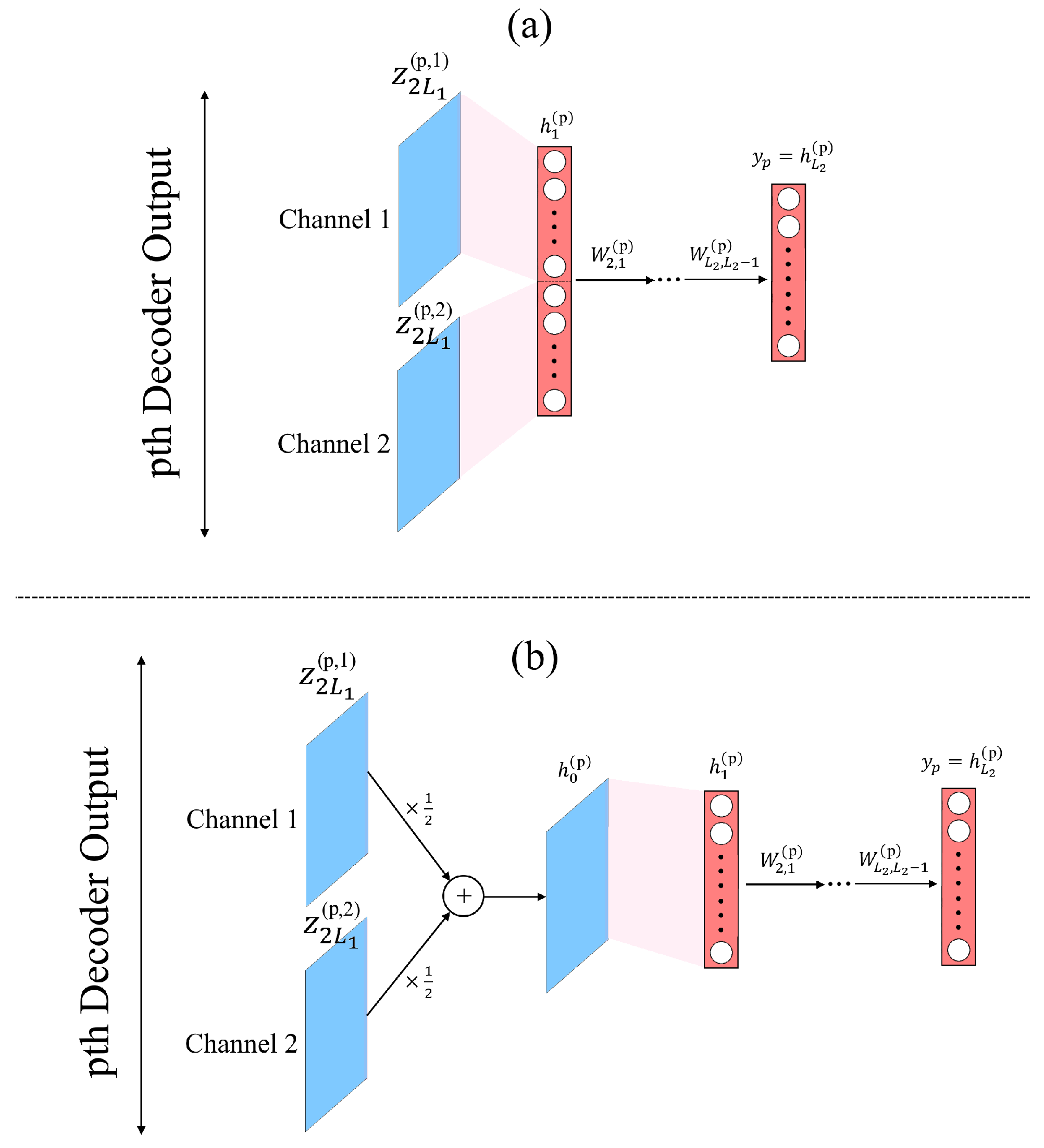
4.3. CAE Multilayer Classifiers

The outputs of the P spatial subregions of the decoder are used as the inputs of the P groups of the parallel multilayer classifiers, and the layers of two channels for each group of classifiers are connected by a fully connected layer neural network. The spatial spectrum of the corresponding subregion is estimated after $L_2$ layers. Finally, the outputs of the P groups of parallel classifiers are combined into $\mathbf{y}$ as written in (17) to determine the direction of the incident signal.

As plotted in Figure 4, the parallel multilayer classifiers in CAE can have two different structures: the first is to directly process the data of the two channels, and the second is to merge the separate channels into one input vector for the classifier, with which the entire feature map has a smaller dimension than the first structure, described as follows:

$$\begin{array}{cc}\hfill {\mathbf{h}}_0^{\left(p\right)}& =({\mathbf{z}}_{2L_1}^{(p,1)}+{\mathbf{z}}_{2L_1}^{(p,2)})/2\hfill \\ & \mathtt{for}p=1,2,\cdots ,P\hfill \end{array}$$

(23)

where ${\mathbf{z}}_{2L_1}^{(p,1)}$ and ${\mathbf{z}}_{2L_1}^{(p,2)}$ denote the two channel outputs associated with the pth convolutional kernel and ${\mathbf{h}}_0^{\left(p\right)}$ is the input of the pth classifier.

5. Numerical Simulations

5.1. Simulation Settings

Table 1. Simulation parameters.

Parameters	Values
number of antennas (M)	10
number of snapshot (N)	512
$N_{\mathrm{trials}}$	10,000
noisy environment	AWGN
spatial scope $[{\theta }^{\left(0\right)},{\theta }^{\left(P\right)})$	$[-{60}^{\circ },{60}^{\circ })$
number of subregion (P)	6
spatial subregion ($I_0$)	20
direction grid	$1^{\circ }$
learning rate ($\eta$)	$0.001$
number of batch size	128
SNR (dB)	10

shows the simulation parameters, with which we simulate a ULA system of $M=10$ antenna elements. The DOA range of the signal source is ${\theta }^{\left(0\right)}=-{60}^{\circ },{\theta }^{\left(P\right)}={60}^{\circ }$, where we divide the ${120}^{\circ }$ spatial range into $P=6$ subregions with each angle interval of $1^{\circ }$ as the classification category (class). Each spatial subregion is then responsible for $I_0=20$ classes. We fix the environmental SNR at 10 dB during training. Usually when using deep learning methods, the entire training set is not directly used as input at once because the amount of data in the training set is huge and exceeds the memory loading of the normal computer. Here, we adopt the minibatch training method, where the entire training set is divided into multiple subset data and each subset size (batch size) is 128. Each training uses only one subset for batch processing. Training each subset in batches is called an epoch, and we repeat the entire training set for 10 epochs. In addition, we apply the stochastic gradient descent method, which is the simplest gradient descent, to find the gradient of the parameters for updating the parameter $\mathbf{W}$ in the direction of the gradient as follows:

$${\mathbf{W}}^{new}={\mathbf{W}}^{old}-\eta \frac{\mathsf{\Delta }Loss}{\mathbf{W}}$$

(24)

where $\eta$ is the learning rate and $\frac{\mathsf{\Delta }Loss}{\mathbf{W}}$ denotes the gradient of the loss function.

In this simulation, we analyze the accuracy of different methods as follows. Suppose we have a test set with a total of $N_{\mathrm{trials}}$ samples. Each sample is systematically tested to obtain the prediction category, and then the real category is compared to judge whether the classification is correct. The number of correctly predicted samples is divided by the total number of samples to calculate the accuracy rate.

5.2. Determination of Main CAE Parameters

Through simulations with varying different parameters, we determine several important system parameters in the proposed CAE structure. We show the performance of the proposed CAE with four major system parameters, including the number of convolutional kernel K, the kernel size $B\times B$, the number of the multitasking AE layers $L_1$, and the number of the parallel multilayer classifier layers $L_2$. With the experiments of varying system parameters, we found that when the complexity of the CAE structure increases, the variables due to the neurons inside the system will increase such that the overfitting problem can decrease accuracy. In some papers, in order to overcome the problem of overfitting, the structure with more layers requires learning more training samples. Here, we use a fixed number of training samples for the comparison of different parameters.

Figure 5a shows the comparison of accuracy with different numbers $L_1=2,3$, and 4 of multitasking AE layers in CAE at SNR ranged from $-10$ dB to 20 dB, where the number of the kernel is set to $K=64$, the kernel size is $2\times 2$, the number of classifier layers is $L_2=5$, and the angle of the incident signal is ${10}^{\circ }$. It can be seen from the figure that when SNR is above 5 dB, the three different layers can achieve an accuracy of nearly 100%. As SNR equals to 0 dB and $-5$ dB, the difference between using two layers and using three layers is not large, but the accuracy of using four layers decreases. When the SNR is less than $-10$ dB, using 3 layers is better than others. Based on this result, we determine $L_1=3$ layers in our CAE structure.

After deciding $L_1$, Figure 5b compares the accuracy of three different kernel sizes for $2\times 2$, $3\times 3$, and $4\times 4$. When SNR is greater than 5 dB, the accuracy of the three sizes is close to 100%, and when SNR is lower than 0 dB, it can be seen that the kernel size $B=2$ is the best to resist noise. The main purpose of the kernel is to learn the characteristics of DOA to understand the correlation between adjacent antennas. From the simulation result, the kernel size in our CAE structure is chosen as $2\times 2$.

Figure 5c compares the accuracy for different numbers of kernels with $K=8$, 16, 32, 64, and 128. When SNR is below 0 dB, it can be seen that the noise is best countered with $K=64$. The appropriate number of kernels is very important because K kernels will produce K feature maps, and if too many feature maps are generated, the system parameters will be too complicated such that overfitting problems occur to decrease accuracy.

Figure 5d compares the numbers of layers $L_2$ for $L_2=4$ (with numbers of nodes 200-512-256-20), $L_2=5$ (with numbers of nodes 200-1024-512-256-20), and $L_2=6$ (with numbers of nodes: 200-1452-1024-512-256-20). When SNR is below 0 dB, the noise resistance of the 6 layers of classifiers is the best. A multilayer classifier is divided into input layer, hidden layer, and output layer, where the number of nodes in input layer is determined by the output of the AE decoder, and the number of nodes in the output layer is judged by the corresponding spatial subregion range $I_0$. Here, we choose $I_0=20$ classes in the output layer. As choosing the numbers of nodes in hidden layers, we reduce the number of nodes layers by layers. According to our experience, if the number of nodes in one layer is suddenly increased or decreased, this may lead to poor results in model training. In this experiment, we set the number of nodes in the first hidden layer to 1452, the second layer 1024, the third layer 512, and the fourth layer 256.

5.3. Accuracy Performance of the CAE Method with Different Parallel Multilayer Classifiers

The performance comparison of two kinds of parallel multilayer classifiers mentioned in Section 3 is that the first treats all the variables of the two channels as input vectors, and the second combines two independent channels into a single channel and then treats the variables of the merged channel as input vectors. The length of the first input vector is 200, and the length of the second input vector is reduced to 100. Figure 6 compares the accuracy of the two methods. When SNR is greater than 0 dB, the accuracy of both classifier methods is almost 100%, and when SNR is at −5 dB, it is better to treat all variables as input vectors from the simulation result. Here, we apply the first method in our CAE structure for comparing the simulation results.

5.4. Performance Comparison of DAE and CAE Methods

We then compare the accuracy of four different deep learning algorithms to determine the DOA of the incident signal: the first is the traditional DNN method, the second is AE without considering subregions, the third is DAE, and the fourth is the proposed CAE. From Figure 7, it can be seen that the third and fourth methods have better accuracy at low SNR than AE without considering subregions, and the proposed CAE also has better noise immunity than DAE.

Next, we analyze the case that two different signal sources exist, and the spatial filter for separating subregions is applied to both the DAE and CAE methods, where the system parameters for DAE and CAE can be referred to in

Table 2. System parameters of the DAE structure.

Parameters	Values
number of AE layers ($L_1$)	3
size of input vector	200
number of classifier layers ($L_2$)	5
loss function	Relu function

and

Table 3. System parameters of the CAE structure.

Parameters	Values
number of AE layers ($L_1$)	3
number of convolution kernel (K)	64
size of input matrix ($A\times A$)	$10\times 10$
size of convolution kernel ($B\times B$)	$2\times 2$
number of classifier layers ($L_2$)	6
loss function	Relu function

, respectively. We separate the spatial range of the signal direction into 6 subregions in $[-{60}^{\circ },{60}^{\circ })$, and hence, there are two possibilities when considering the locations of multiple targets. Figure 8a is the comparison of simulating two signal sources located in the same subregion. We assume two similar angles to test the performance results of CAE and DAE; the incident angles of the two signal sources are ${\theta }_1={10}^{\circ }$ and ${\theta }_1={12}^{\circ }$, where the two angles differ by $2^{\circ }$. In the previous CAE result, the accuracy of a single incident signal at 0 dB was as high as 100%. However, when two targets are in the same subregion, as shown in Figure 8a, the accuracy is reduced. Figure 8b is a comparison of simulating two signal sources located in different subregions. We assume two angles with larger difference for testing, and the incident angles of the two signal sources are ${\theta }_1={10}^{\circ }$ and ${\theta }_1={30}^{\circ }$, where the difference between the two angles is ${20}^{\circ }$. With the CAE, the accuracy of both a single signal source and two signal sources at 5 dB SNR can reach almost 100%. From the figure, we can see that when the two angles are located in different subregions, the CAE performance is still close to that of a single signal source. Although the accuracy of DAE does not decrease in the case of high SNR, CAE has better results than DAE in the case of low SNR. From this experiment, we can find that when we consider multiple targets, the difficulty of DOA estimation increases, and the proposed CAE has obvious advantages.

5.5. RMSE Performance Comparison of DOA Estimation with Array Imperfections

Before applying the CAE to deal with the array imperfections problem, we first show the confusion matrix for accuracy analysis of DOA estimation at 10 dB SNR based on the previously established parameters as listed in Table 3. We test the proposed CAE method by randomly generating test samples of the incident angle ranged from $-{60}^{\circ }$ to ${60}^{\circ }$ with the amount of 100 data per $1^{\circ }$. The real category of each test sample and the predicted category are accumulated to produce the confusion matrix. Figure 9 shows the matrices for the 6 subregions, where the darker the blue inside the lattice, the higher the accuracy rate represented. We can find that the determined DOA grid and the true value almost coincide, that is, with the proposed CAE in the absence of array imperfections, the accuracy of DOA estimation within $1^{\circ }$ error at 10 dB SNR is almost close to $100\%$.

Next, considering the parameters of array imperfections as listed in

Table 4. Simulation parameters of array imperfections.

Parameters	Values
gain biases ($0,{\gamma }_{gain}^{\left(1\right)},\cdots ,{\gamma }_{gain}^{(M-1)}$)	$\begin{array}{ccc}0,& \underset{\underset{5}{︸}}{\begin{array}{ccc}0.2,& \cdots ,& 0.2,\end{array}}& \underset{\underset{4}{︸}}{\begin{array}{ccc}-0.2,& \cdots ,& -0.2\end{array}}\end{array}$
phase biases ($0,{\gamma }_{phase}^{\left(1\right)},\cdots ,{\gamma }_{phase}^{(M-1)}$)	$\begin{array}{ccc}0,& \underset{\underset{5}{︸}}{\begin{array}{ccc}{30}^{\circ },& \cdots ,& {30}^{\circ },\end{array}}& \underset{\underset{4}{︸}}{\begin{array}{ccc}-{30}^{\circ },& \cdots ,& -{30}^{\circ }\end{array}}\end{array}$
position errors ($0,{\gamma }_{pos}^{\left(1\right)},\cdots ,{\gamma }_{pos}^{(M-1)}$)	$\begin{array}{ccc}0,& \underset{\underset{5}{︸}}{\begin{array}{ccc}0.2,& \cdots ,& 0.2,\end{array}}& \underset{\underset{4}{︸}}{\begin{array}{ccc}-0.2,& \cdots ,& -0.2\end{array}}\end{array}$
mutual coupling coefficient (${\gamma }_{mc}$)	$0.3e^{j{60}^{\circ }}$

, we analyze the RMSE performance of DOA estimation with the proposed CAE method, and compare the result of CAE with those of ESPRIT and DAE. Assume that the incident angle is randomly generated between $9.5^{\circ }$ and $10.5^{\circ }$, SNR is fixed at 10 dB, and the imperfection control parameter $\rho$ varies between 0 and 1. The larger $\rho$ means that the deviation from the ideal imperfection-free array is greater, and $\rho =0$ means that the array is ideal. Figure 10 show four different array imperfection cases. Figure 10a adds only gain and phase deviations to the array. Figure 10b considers the antenna coupling effect, Figure 10c considers the error influence in the antenna position, and Figure 10d combines the three array imperfections at the same time. From the results of these experiments, it can be found that when the array is ideal, the ESPRIT algorithm can obtain a very high resolution. The classical ESPRIT algorithm similar to the MUSIC algorithm used in [9] is the subspace-based high resolution method for DOA estimation and in contrast, has the advantage of significantly reducing the computing power and memory needed for storage. However, ESPRIT is developed based on the ideal array responding function and exploits the property of the translational invariance of the antenna array by decomposing the array into two sub-networks of identical antennas, in which one can be obtained by a translation of the other. Hence, increasing $\rho$ will degrade the performance of ESPRIT. Since DAE and CAE methods do not rely on the geometry of the antenna or any assumption about the antenna models, they can adapt to different kinds of array imperfections. DOA estimation based on the deep learning methods does not fluctuate sharply with the influence of array imperfections.

In Figure 11, we show the comparison of DOA prediction for DAE and CAE with all DOA training ranges $[-{60}^{\circ },{60}^{\circ })$ at SNR of 5 dB and 10 dB. As the results shown in Figure 10d and Figure 11b, DAE and CAE have no significant difference at 10 dB SNR. However, for the SNR value reduced to 5 dB, the accuracy of DOA prediction for DAE becomes worse while CAE remains a satisfying accuracy. This result can be obviously observed from Figure 7, showing that at 0 dB SNR, the accuracy of DAE dramatically drops to $30\%$, while CAE almost has a satisfying result. In Figure 11a at 5 dB SNR, an obvious accuracy loss appears for DAE performing with combined array imperfections.

6. Conclusions

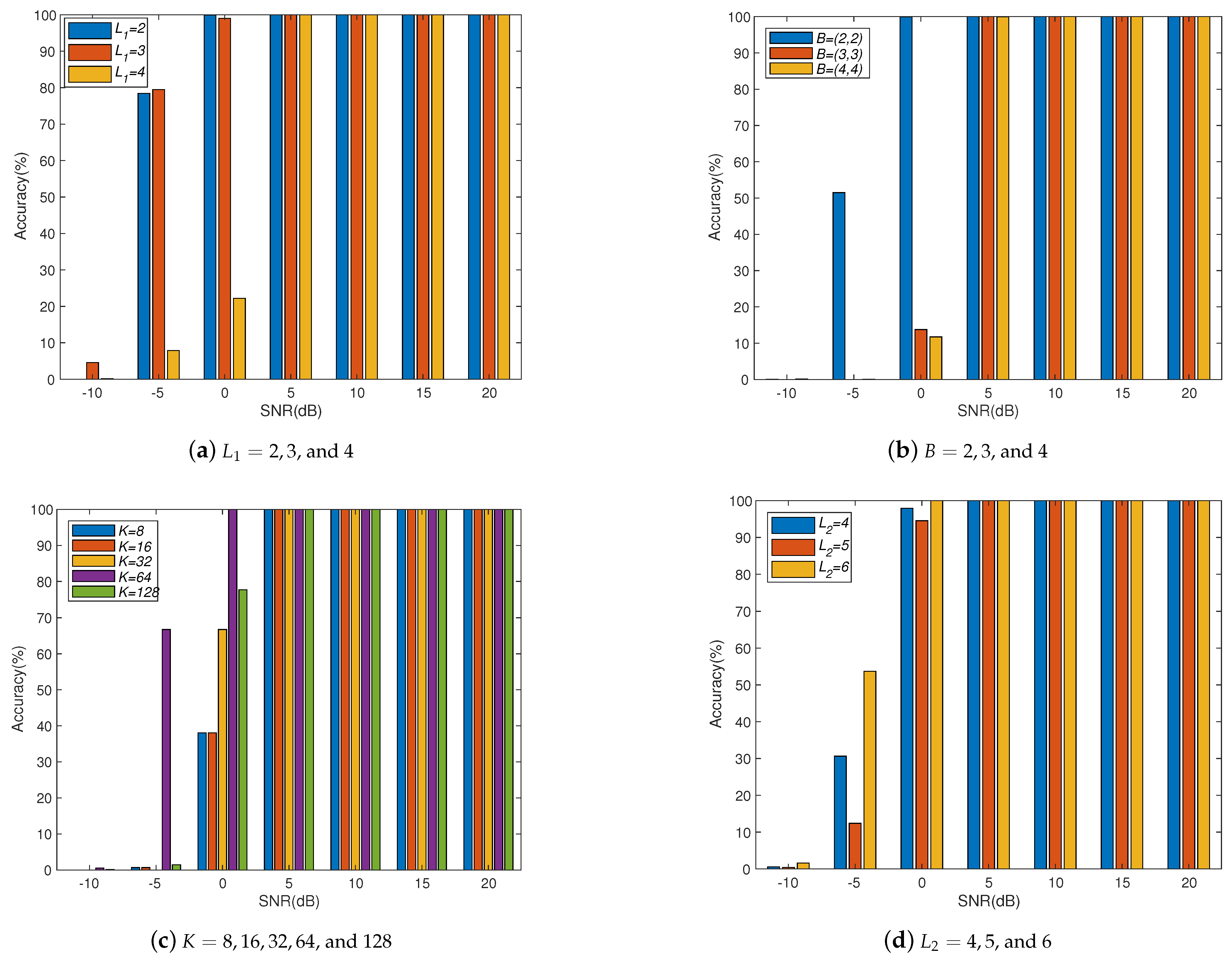
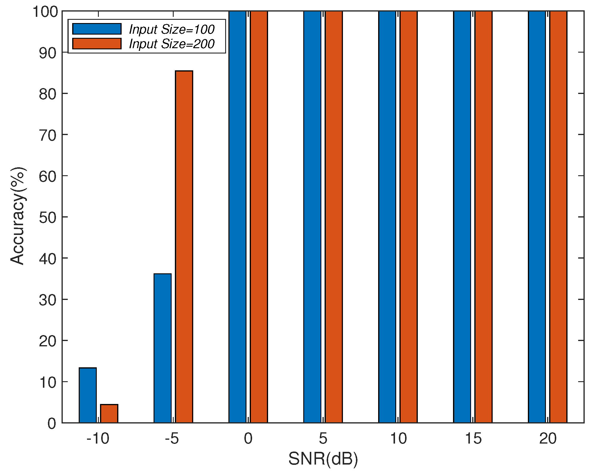
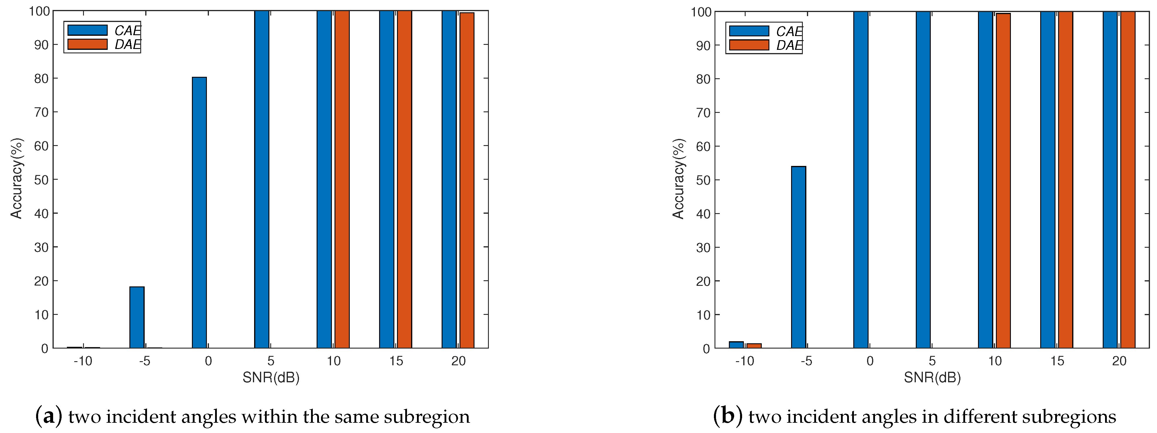
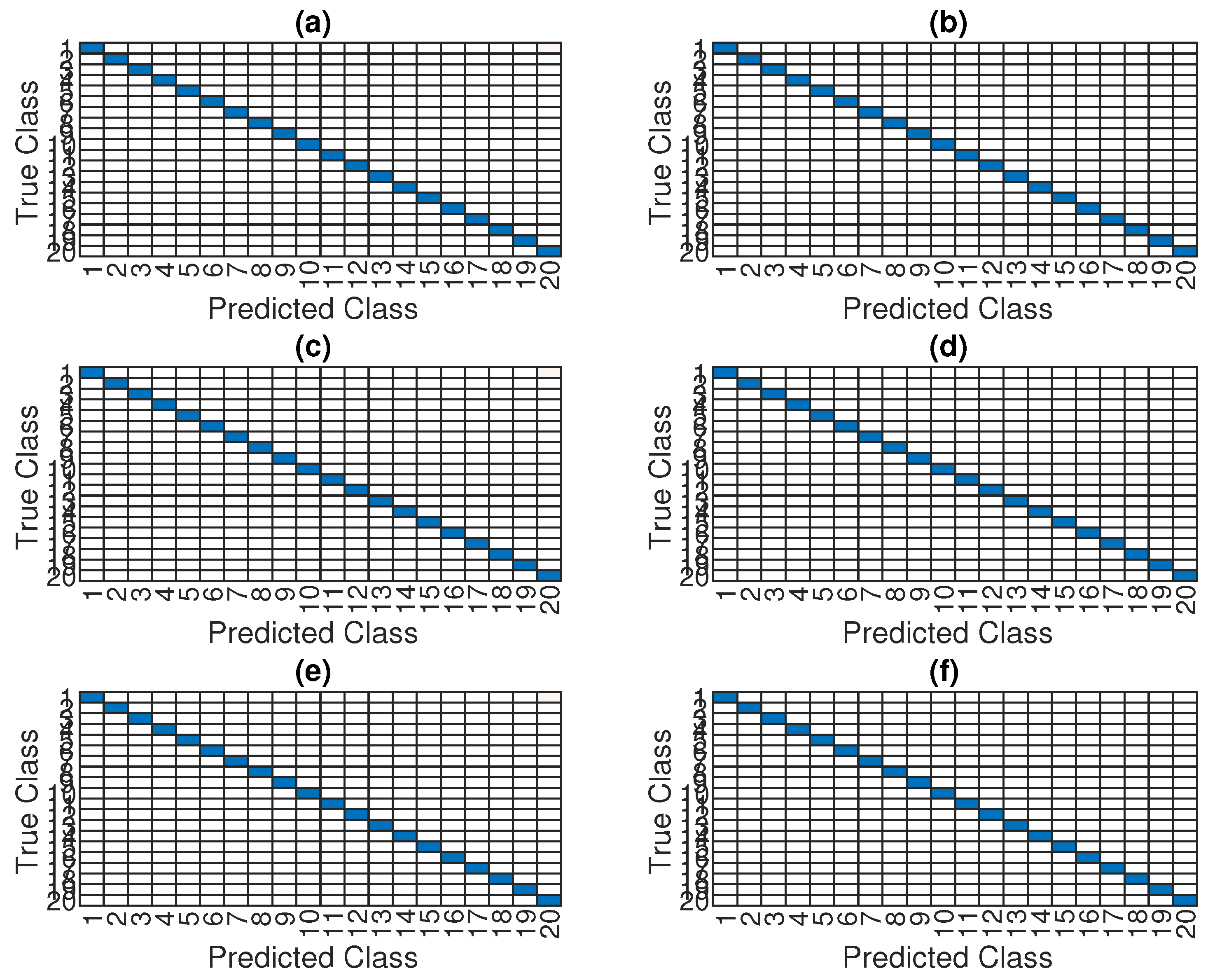
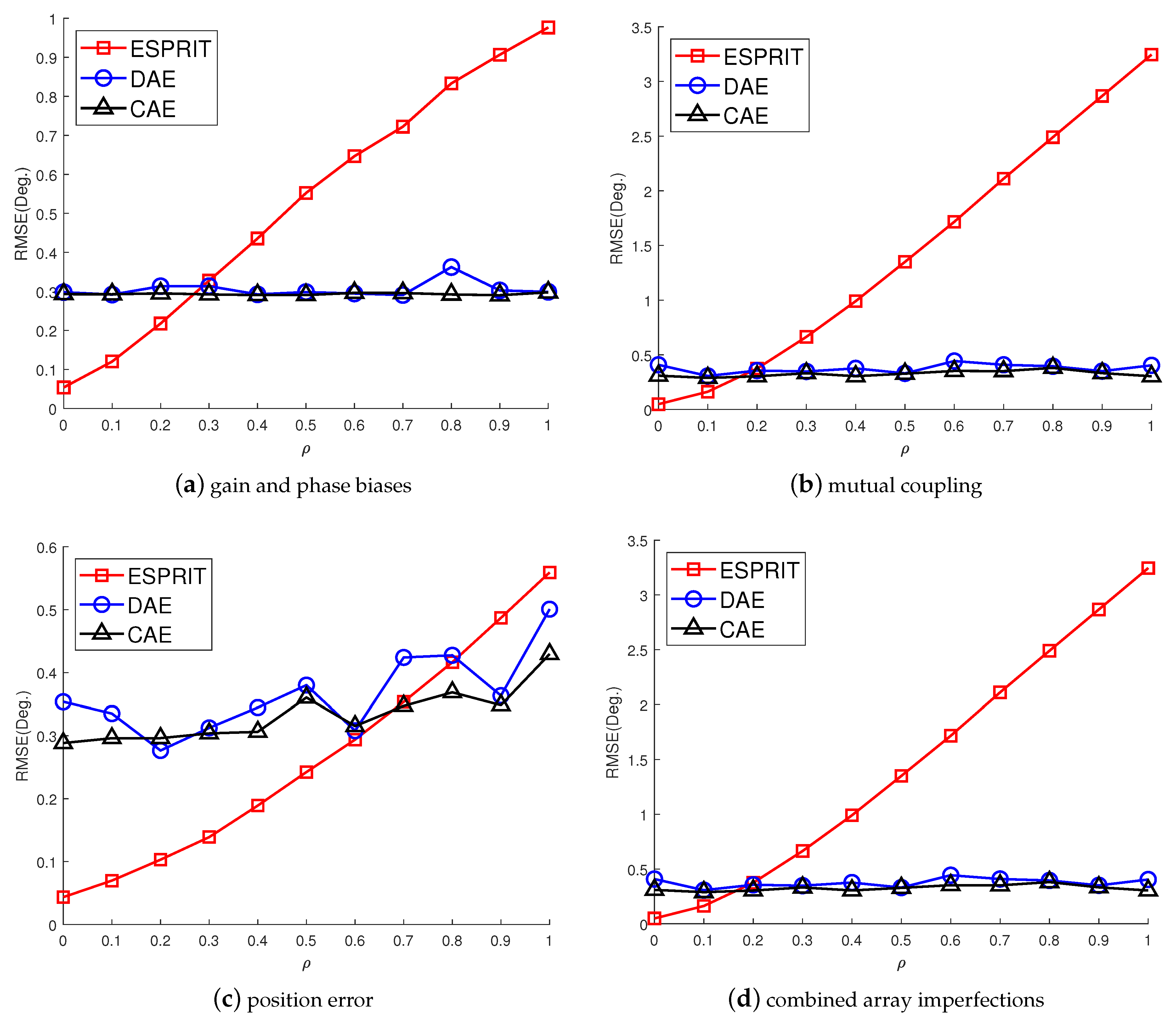
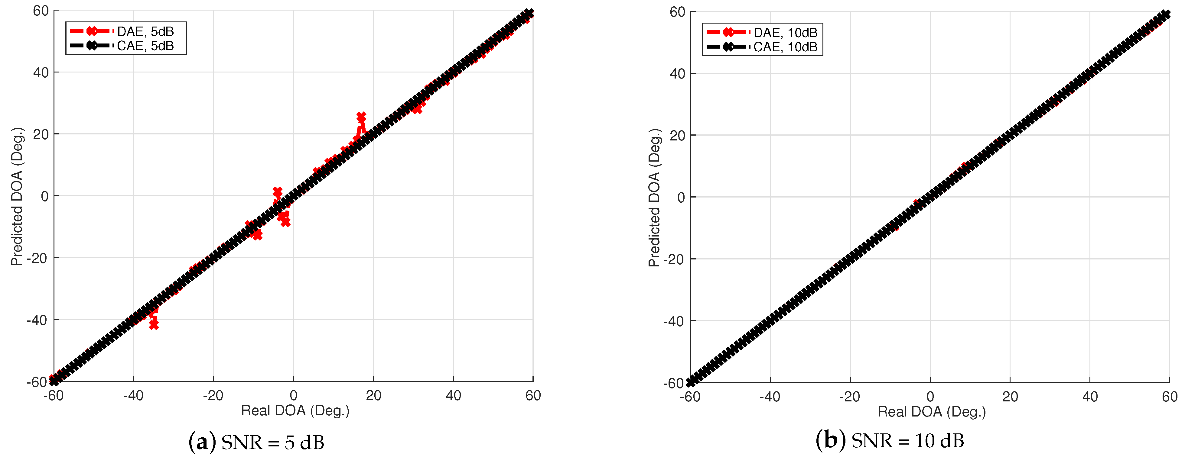
We study a CAE structure to deal with array imperfections for obtaining robust DOA estimation, which combines the advantages of convolutional operations to learn local spatial features and the use of spatial filters to concentrate the training information. Through numerical experiments, we study different system parameters to improve system accuracy with the proposed CAE. In the case of increasing the number of layers in CAE, the overall accuracy will not be improved due to the overfitting effect. Therefore, the CAE parameters need to be properly determined to obtain better accuracy with reasonable training load according to the applications. In addition, we also show the performance of the proposed CAE method with multiple signal sources. When multiple signal sources occur in different subregions, the performance of the proposed CAE is still similar to that of a single source. After evaluating the noise immunity performance of the DNN, DAE, and CAE methods, we find out that CAE has better noise immunity than others. Although deep learning methods for DOA estimation are inferior to subspace-based methods, such as MUSIC and ESPRIT, without array imperfections, the performance is worse due to the resolution limitation of the finite output grids of the multilayer classifiers. The proposed CAE method demonstrates a robust performance in solving complex array imperfection problems.

References

1. Schmidt, R. Multiple emitter location and signal parameter estimation. IEEE Trans. Antennas Propag. 1986, 34, 276–280. [Google Scholar] [CrossRef]
2. Yuen, N.; Friedlander, B. Asymptotic performance analysis of ESPRIT, higher order ESPRIT, and virtual ESPRIT algorithms. IEEE Trans. Signal Process. 1996, 44, 2537–2550. [Google Scholar] [CrossRef]
3. Yan, F.; Jin, M.; Qiao, X. Low-Complexity DOA Estimation Based on Compressed MUSIC and Its Performance Analysis. IEEE Trans. Signal Process. 2013, 61, 1915–1930. [Google Scholar] [CrossRef]
4. Tan, Z.; Eldar, Y.C.; Nehorai, A. Direction of Arrival Estimation Using Co-Prime Arrays: A Super Resolution Viewpoint. IEEE Trans. Signal Process. 2014, 62, 5565–5576. [Google Scholar] [CrossRef]
5. Gao, F.; Gershman, A. A generalized ESPRIT approach to direction-of-arrival estimation. IEEE Signal Process. Lett. 2005, 12, 254–257. [Google Scholar] [CrossRef]
6. Zhang, W.; Han, Y.; Jin, M.; Li, X.S. An Improved ESPRIT-Like Algorithm for Coherent Signals DOA Estimation. IEEE Commun. Lett. 2020, 24, 339–343. [Google Scholar] [CrossRef]
7. Jablon, N. Adaptive beamforming with the generalized sidelobe canceller in the presence of array imperfections. IEEE Trans. Antennas Propag. 1986, 34, 996–1012. [Google Scholar] [CrossRef]
8. Friedlander, B.; Weiss, A.J. Direction finding in the presence of mutual coupling. IEEE Trans. Antennas Propag. 1991, 39, 273–284. [Google Scholar] [CrossRef]
9. Liu, Z.; Zhang, C.; Yu, P.S. Direction-of-Arrival Estimation Based on Deep Neural Networks With Robustness to Array Imperfections. IEEE Trans. Antennas Propag. 2018, 66, 7315–7327. [Google Scholar] [CrossRef]
10. Viberg, M.; Swindlehurst, A.L. Analysis of the combined effects of finite samples and model errors on array processing performance. IEEE Trans. Signal Process. 1994, 42, 3073–3083. [Google Scholar] [CrossRef] [Green Version]
11. Xie, W.; Wang, C.; Wen, F.; Liu, J.; Wan, Q. DOA and Gain-Phase Errors Estimation for Noncircular Sources With Central Symmetric Array. IEEE Sens. J. 2017, 17, 3068–3078. [Google Scholar] [CrossRef]
12. Porat, B.; Friedlander, B. Accuracy requirements in off-line array calibration. IEEE Trans. Aerosp. Electron. Syst. 1997, 33, 545–556. [Google Scholar] [CrossRef]
13. Pastorino, M.; Randazzo, A. A smart antenna system for direction of arrival estimation based on a support vector regression. IEEE Trans. Antennas Propag. 2005, 53, 2161–2168. [Google Scholar] [CrossRef]
14. Randazzo, A.; Abou-Khousa, M.A.; Pastorino, M.; Zoughi, R. Direction of Arrival Estimation Based on Support Vector Regression: Experimental Validation and Comparison with MUSIC. IEEE Antennas Wirel. Propag. Lett. 2007, 6, 379–382. [Google Scholar] [CrossRef]
15. Xiao, X.; Zhao, S.; Zhong, X.; Jones, D.L.; Chng, E.S.; Li, H. A learning-based approach to direction of arrival estimation in noisy and reverberant environments. In Proceedings of the 2015 IEEE International Conference on Acoustics, Speech and Signal Processing (ICASSP), South Brisbane, Australia, 19–24 April 2015; pp. 2814–2818. [Google Scholar]
16. Vesperini, F.; Vecchiotti, P.; Principi, E.; Squartini, S.; Piazza, F. A neural network based algorithm for speaker localization in a multi-room environment. In Proceedings of the 2016 IEEE 26th International Workshop on Machine Learning for Signal Processing (MLSP), Salerno, Italy, 13–16 September 2016; pp. 1–6. [Google Scholar]
17. Chakrabarty, S.; Habets, E.A.P. Multi-Speaker DOA Estimation Using Deep Convolutional Networks Trained With Noise Signals. IEEE J. Sel. Top. Signal Process. 2019, 13, 8–21. [Google Scholar] [CrossRef]
18. Liu, Z.M.; Zhou, Y.Y. A Unified Framework and Sparse Bayesian Perspective for Direction-of-Arrival Estimation in the Presence of Array Imperfections. IEEE Trans. Signal Process. 2013, 61, 3786–3798. [Google Scholar] [CrossRef]
19. Wang, M.; Ma, X.; Yan, S.; Hao, C. An Autocalibration Algorithm for Uniform Circular Array With Unknown Mutual Coupling. IEEE Antennas Wirel. Propag. Lett. 2016, 15, 12–15. [Google Scholar] [CrossRef]
20. Dai, Z.; Su, W.; Gu, H. A Gain and Phase Autocalibration Approach for Large-Scale Planar Antenna Arrays. IEEE Commun. Lett. 2021, 25, 1645–1649. [Google Scholar] [CrossRef]
21. Wang, J.; Zhang, X.; Gao, Q.; Yue, H.; Wang, H. Device-Free Wireless Localization and Activity Recognition: A Deep Learning Approach. IEEE Trans. Veh. Technol. 2017, 66, 6258–6267. [Google Scholar] [CrossRef]
22. Zhao, L.; Huang, H.; Li, X.; Ding, S.; Zhao, H.; Han, Z. An Accurate and Robust Approach of Device-Free Localization With Convolutional Autoencoder. IEEE Internet Things J. 2019, 6, 5825–5840. [Google Scholar] [CrossRef]
23. Xiao, C.; Yang, D.; Chen, Z.; Tan, G. 3-D BLE Indoor Localization Based on Denoising Autoencoder. IEEE Access 2017, 5, 12751–12760. [Google Scholar] [CrossRef]
24. Seong, J.H.; Seo, D.H. Selective Unsupervised Learning-Based Wi-Fi Fingerprint System Using Autoencoder and GAN. IEEE Internet Things J. 2020, 7, 1898–1909. [Google Scholar] [CrossRef]
25. Ahmed, A.M.; Eissa, O.; Sezgin, A. Deep Autoencoders for DOA Estimation of Coherent Sources using Imperfect Antenna Array. In Proceedings of the 2020 Third International Workshop on Mobile Terahertz Systems (IWMTS), Essen, Germany, 1–2 July 2020; pp. 1–5. [Google Scholar] [CrossRef]
26. Fang, W.; Cao, Z.; Yu, D.; Wang, X.; Ma, Z.; Lan, B.; Song, C.; Xu, Z. A Lightweight Deep Learning-Based Algorithm for Array Imperfection Correction and DOA Estimation. J. Commun. Inf. Netw. 2022, 7, 296–308. [Google Scholar] [CrossRef]
27. Ji, Y.; Wen, C.; Huang, Y.; Peng, J.; Fan, J. Robust direction-of-arrival estimation approach using beamspace-based deep neural networks with array imperfections and element failure. IET Radar Sonar Navig. 2022, 16, 1761–1778. [Google Scholar] [CrossRef]
28. Elbir, A.M. A Novel Data Transformation Approach for DOA Estimation with 3-D Antenna Arrays in the Presence of Mutual Coupling. IEEE Antennas Wirel. Propag. Lett. 2017, 16, 2118–2121. [Google Scholar] [CrossRef]
29. Wang, W.; Wu, R.; Liang, J.; So, H.C. Phase Retrieval Approach for DOA Estimation With Array Errors. IEEE Trans. Aerosp. Electron. Syst. 2017, 53, 2610–2620. [Google Scholar] [CrossRef]
30. Forster, P. Generalized rectification of cross spectral matrices for arrays of arbitrary geometry. IEEE Trans. Signal Process. 2001, 49, 972–978. [Google Scholar] [CrossRef]
Figure 1. M-antenna ULA structure.
Electronics 12 00771 g001
Figure 2. Deep neural network autoencoder structure [9] for DOA estimation.
Electronics 12 00771 g002
Figure 3. The proposed convolutional autoencoder structure for DOA estimation.
Electronics 12 00771 g003
Figure 4. Two different structures of parallel multilayer classifiers in proposed CAE for DOA estimation: (a) the structure of direct processing of two channels, (b) the structure of merging two channels.
Electronics 12 00771 g004
Figure 5. The influence of four CAE parameters on performance: (a) accuracy of different numbers of encoding layers L 1 versus SNR, (b) accuracy of different kernel sizes B × B versus SNR, (c) accuracy of different numbers of kernel K versus SNR, (d) accuracy of different numbers of decoding layers L 2 versus SNR.
Electronics 12 00771 g005
Figure 6. Comparison of accuracy with different input sizes for the parallel multilayer classifiers in CAE.
Electronics 12 00771 g006
Figure 7. Comparison of accuracy with different deep learning methods for DOA estimation.
Electronics 12 00771 g007
Figure 8. Performance comparison of DAE and CAE with two different signal sources: (a) accuracy of two incident angles θ 1 = 10 and θ 1 = 12 within the same subregion versus SNR, (b) accuracy of two incident angles θ 1 = 10 and θ 1 = 30 in different subregions versus SNR.
Electronics 12 00771 g008
Figure 9. Confusion matrix of the CAE method for output angles versus incident angles at 10 dB SNR: (a) the subregion of the incident angle in [−60, −40), (b) the subregion of the incident angle in [−40, −20), (c) the subregion of the incident angle in [−20, 0), (d) the subregion of the incident angle in [0, 20), (e) the subregion of the incident angle in [20, 40), (f) the subregion of the incident angle in [40, 60).
Electronics 12 00771 g009
Figure 10. RMSE performance of DOA estimation for ESPRIT, DAE, and CAE methods with different array imperfections versus the imperfection control parameter ρ at 10 dB SNR: (a) antenna gain and phase biases, (b) antenna mutual coupling, (c) antenna position error, (d) combined array imperfections.
Electronics 12 00771 g010
Figure 11. DOA prediction of DAE and CAE performed with combined array imperfections: (a) SNR = 5 dB, (b) SNR = 10 dB.
Electronics 12 00771 g011