Improved Salp Swarm Algorithm for Tool Wear Prediction

Abstract

To address the defects of the salp swarm algorithm (SSA) such as the slow convergence speed and ease of falling into a local minimum, a new salp swarm algorithm combining chaotic mapping and decay factor is proposed and combined with back propagation (BP) neural network to achieve an effective prediction of tool wear. Firstly, the chaotic mapping is used to enhance the formation of the population, which facilitates the iterative search and reduces the trapping in the local optimum; secondly, the decay factor is introduced to improve the update of the followers so that the followers can be updated adaptively with the iterations, and the theoretical analysis and validation of the improved SSA are carried out using benchmark test functions. Finally, the improved SSA with a strong optimization capability to solve BP neural networks for the optimal values of hyperparameters is used. The validity of this is verified by using the actual tool wear data set. The test results of the benchmark test function show that the algorithm presented has a better convergence speed and solution accuracy. Meanwhile, compared with the original algorithm, the R² value of the part life prediction model proposed is improved from 0.962 to 0.989, the MSE value is reduced from the original 34.4 to 9.36, which is a 72% improvement compared with the original algorithm, and a better prediction capability is obtained.

1. Introduction

With the advent of the age of massive industrial data, in order to guarantee the highly dependable operation of industrial manufacturing equipment, the remaining life prediction of important parts has received extensive attention from scholars. In the context of tool condition monitoring for metal-cutting operations, the most challenging job is the surveillance of tool wear [1]. Accurately estimating the wear phenomenon of the tool is of great significance in improving production efficiency and reducing processing costs. Therefore, this paper takes the tool wear problem as an example to explore the life prediction problem of mechanical parts.

In recent years, Back Propagation (BP) neural networks, Convolutional Neural Networks (CNN) [2,3], Recurrent Neural Networks (RNN) [4,5], and other deep learning models [6] have been widely adopted due to their ability to handle data nonlinearly. Many neural network-based models have been presented for various aspects of tool wear prediction. Yu et al. [7] presented a method for tool wear monitoring using a weighted Hidden Markov Model with the signals provided by tool condition monitoring techniques. Lin et al. [8] proposed a hidden semi-Markov model for real-time tool wear prediction based on learning for tool wear detection and remaining life prediction. Duan et al. [9] used a parallel deep learning model based on a hybrid attention mechanism to learn sensitive features individually or sequentially from many samples for tool state monitoring. To forecast tool wear, He et al. [10] presented a superimposed sparse autoencoder model based on the BP of the raw temperature signal. F. J. Alonso et al. [11] used feedforward BP neural network technology to predict tool flank wear, but the accuracy of the prediction effect was not high.

To further improve the accuracy of the model prediction, further optimization is required. Metaheuristic algorithms are widely popular optimization algorithms. Metaheuristic methods are divided into nine different groups: biology-based, physics-based, social-based, music-based, chemical-based, sport-based, mathematics-based, swarm-based, and hybrid methods which are combinations of these [12]. Metaheuristic algorithms can be used to solve high-dimensional complex engineering structure optimization design problems with nonlinear constraints. Deng et al. [13] proposed an improved quantum-inspired differential evolution (MSIQDE) algorithm and combined it with a deep belief network (DBN) to propose a fault classification method with a better classification accuracy. Using the elastic net wide learning system (ENBLS) and the grey wolf optimization (GWO) algorithm, Zhao et al. [14] established a unique technique for predicting bearing performance trends. Their method was based on the combination of these two algorithms. The proposed method combined the ENBLS and GWO algorithms to achieve better results. Zhao et al. [15] proposed a novel vibration amplitude spectrum imaging feature extraction method. They compared it with other methods, and the experiment showed that the presented method achieved significant improvements. Huang et al. [16] developed a novel three-phase coevolutionary method to enhance the convergence and searchability of competitive swarm optimizers by combining a novel multi-phase coevolutionary technique. They used it to solve large-scale optimization problems, and the experiments showed that the proposed method obtained better results.

Salp swarm algorithm (SSA) [17] is a swarm-based metaheuristic algorithm that Mirjalili and other scholars in 2017 proposed. Due to its simple and easy framework, few parameters, and good optimization performance compared to other algorithms, it has been widely used in feature selection [18], image processing [19,20,21], engineering optimization [22,23,24], and training neural networks in recent years. It is mostly used to identify various ideal decisions or values to provide a candidate solution that solves the issue [25]. However, many metaheuristic algorithms have shortcomings when faced with multi-dimensional problems, such as slow convergence speed and poor optimization accuracy. Many scholars have made many bold attempts to improve the algorithm. D. Bairathi et al. [26] used the multi-leader SSA to train a feedforward neural network. It analyzed 13 different data sets, proving the ability of the model to gravitate to the optimal value. S. Kassaymeh et al. [27] combined the SSA with the simulated annealing algorithm to optimize hyperparameters of the BP neural network, reduce the model prediction error, and improve the prediction accuracy. J. S. Pan et al. [28] proposed an adaptive multi-group SSA with three new communication strategies, combined it with wind power prediction based on BP, and achieved a nice wind power prediction effect. S. Kassaymeh et al. [29] combined the SSA algorithm with an artificial neural network to optimize network parameters to solve the prediction problem of software testing team size, and evaluated two datasets, showing that the improved method was superior to other methods. M. Zivkovic et al. [30] presented an improved SSA, which firstly combined the exploration and replacement mechanism into the SSA and combined it with another meta-heuristic algorithm. Through the CEC2013 benchmark test, it was verified that the improved algorithm outperformed other more competitive metaheuristic algorithms. Zhang et al. [31] obtained an improved spiral chaotic salp group algorithm by introducing the logarithmic spiral mechanism and combining the chaos search method, which made the development and search capabilities of the algorithm more balanced and further improved the performance of the algorithm. M. H. Qais et al. [32] improved the crucial parameters in the leader’s position update and added random parameters to the follower’s position update mechanism to facilitate the algorithm to obtain the global optimum. Fan et al. [33] used Gaussian perturbation to increase the diversity, introduced polynomial mutation to update the leader position, and used the Laplacian crossover operator and mixed opposition learning method to boost algorithm convergence and exploratory power.

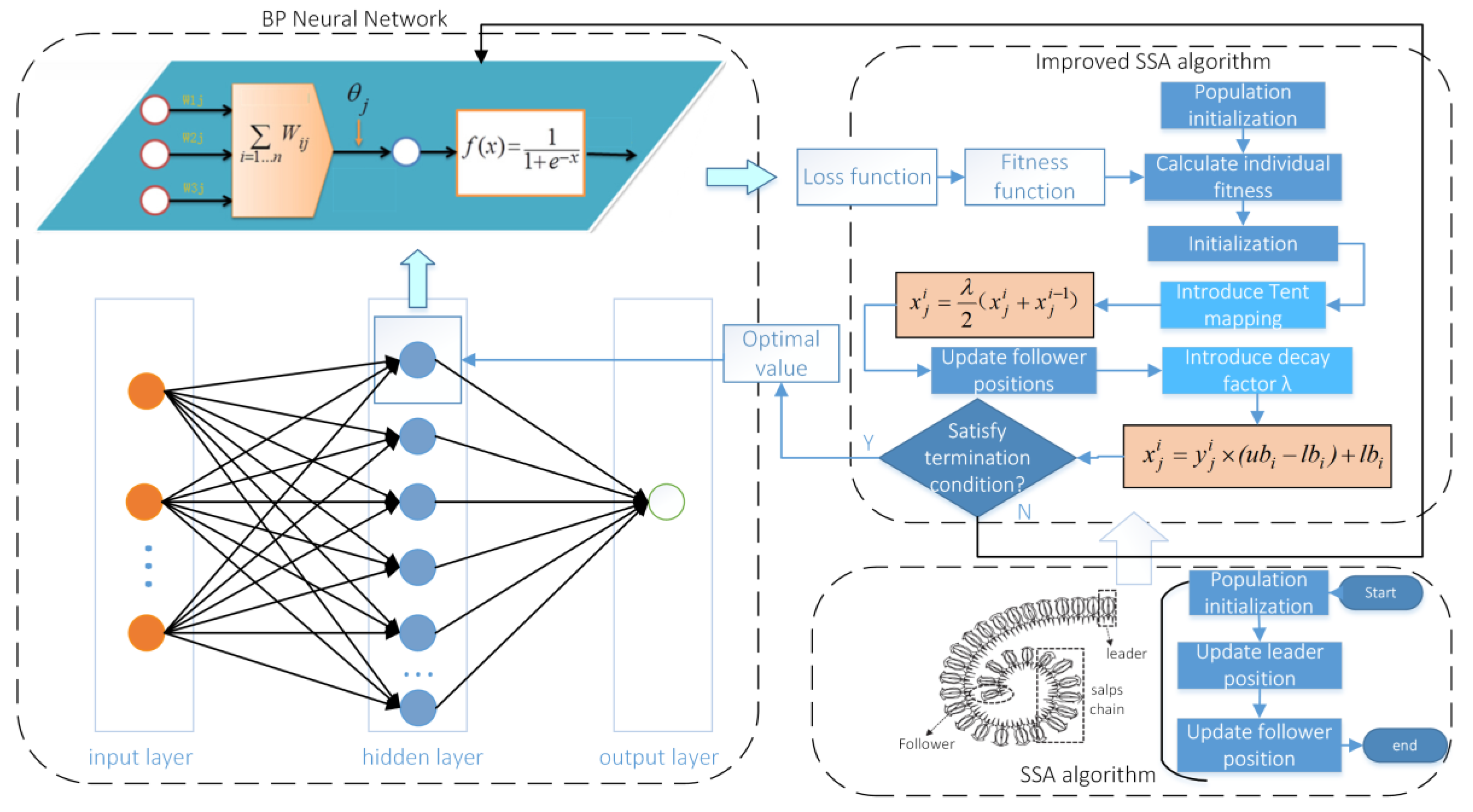
Thus, due to the defects of the salp swarm algorithm such as slow convergence speed and ability to easily fall into local minimum, a new salp swarm algorithm combining chaotic mapping and decay factor is proposed. Considering that the solution accuracy of the neural network is greatly influenced by the relevant initial parameters, the new SSA optimized BP neural network is used to further improve the prediction performance and achieve effective prediction of tool wear. Firstly, the chaotic mapping is used to enhance the formation, which facilitates the iterative search and reduces the trapping in the local optimum; secondly, the decay factor is introduced to improve the update of the followers so that the followers can be updated adaptively with the iterations, and the theoretical analysis and validation of the improved SSA are carried out using benchmark test functions. Finally, the improved SSA with a strong optimization capability is used to solve BP neural networks for optimal values of the hyperparameters. The validity of this is verified by using the actual tool wear data set.

The following are all this paper’s key contributions:

• A new salp swarm algorithm for chaotic mapping and decay factor is presented;
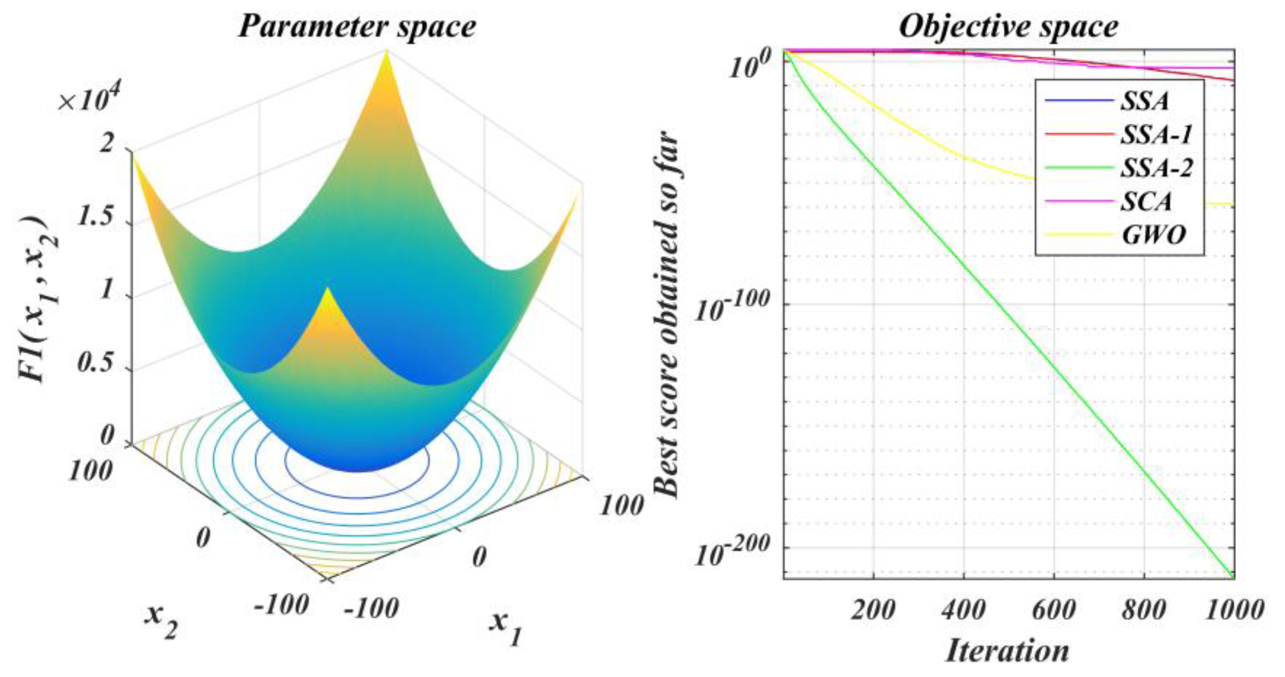
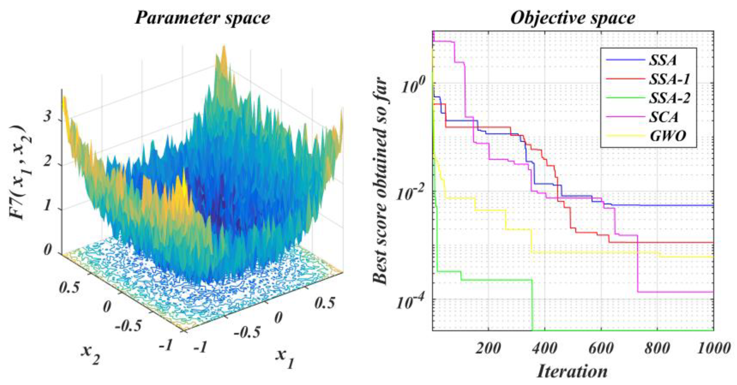
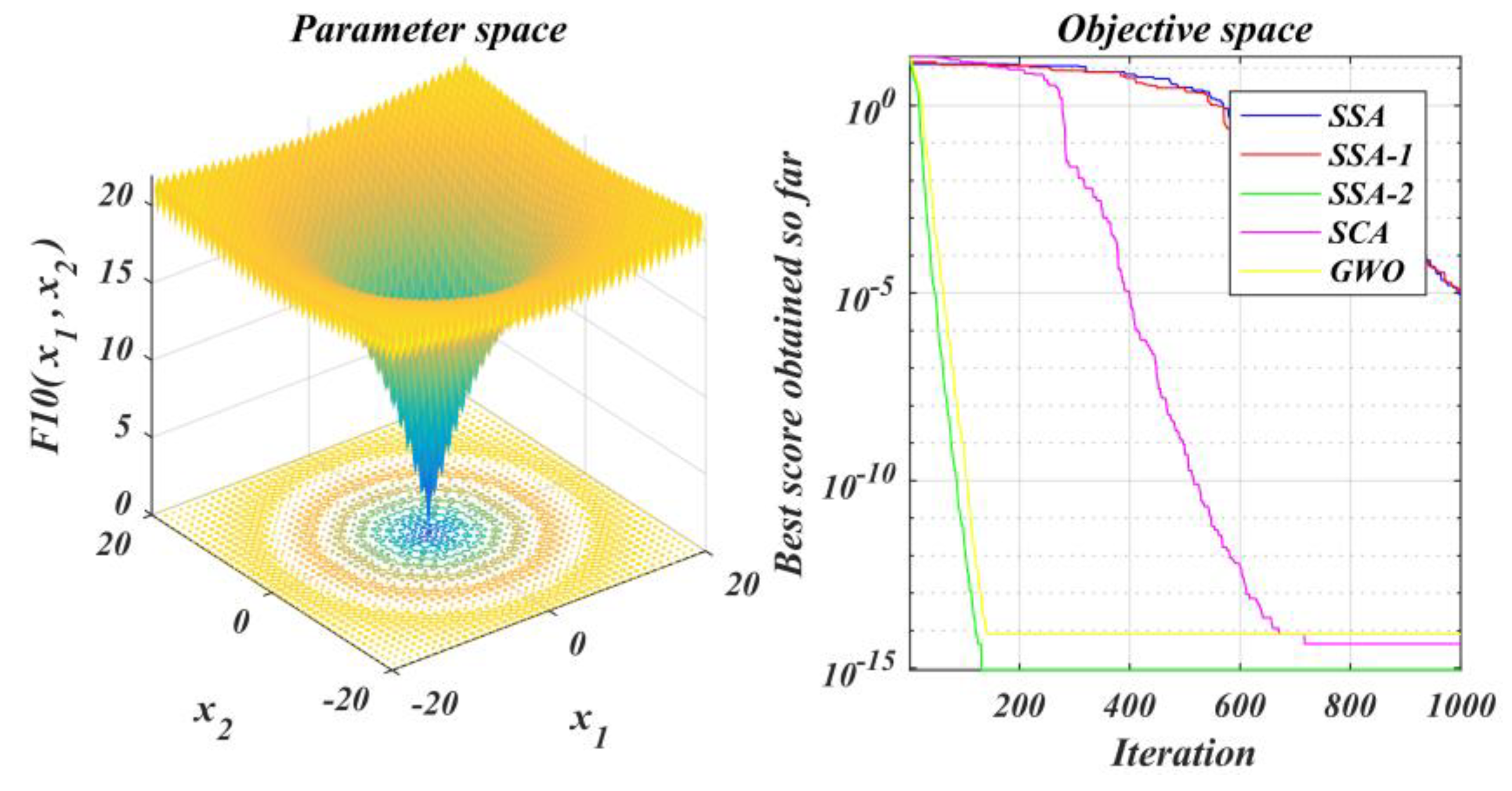
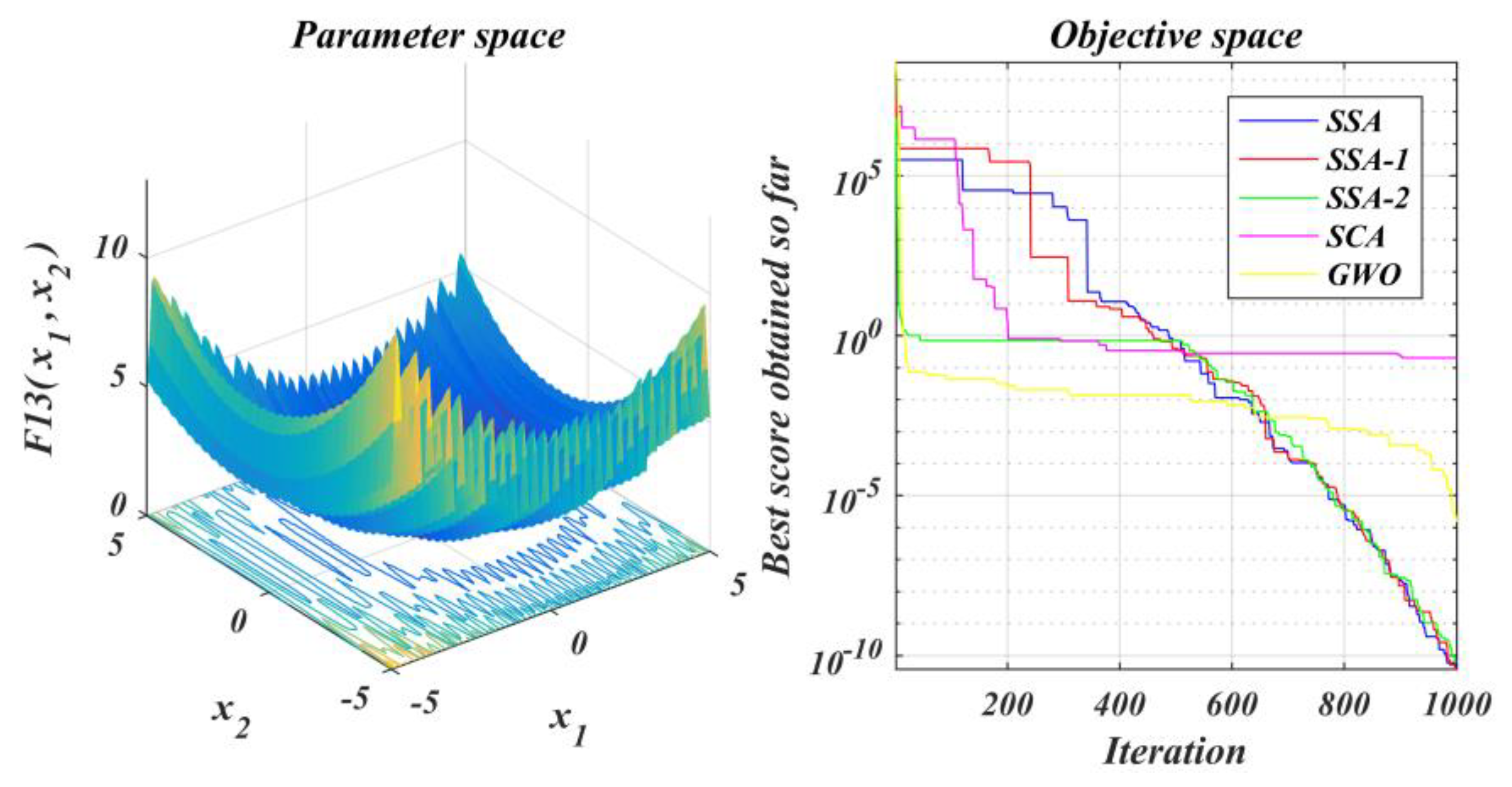
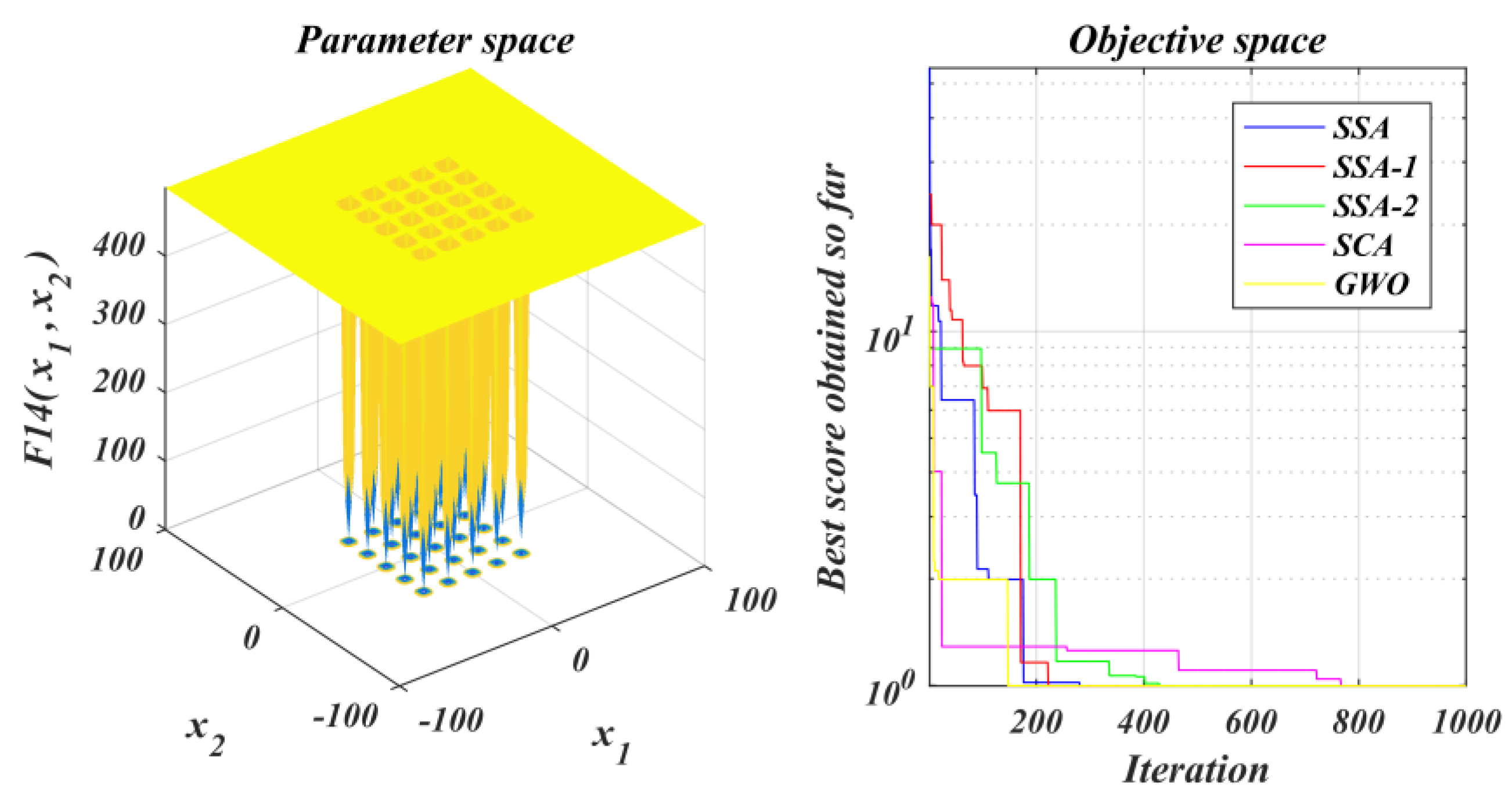
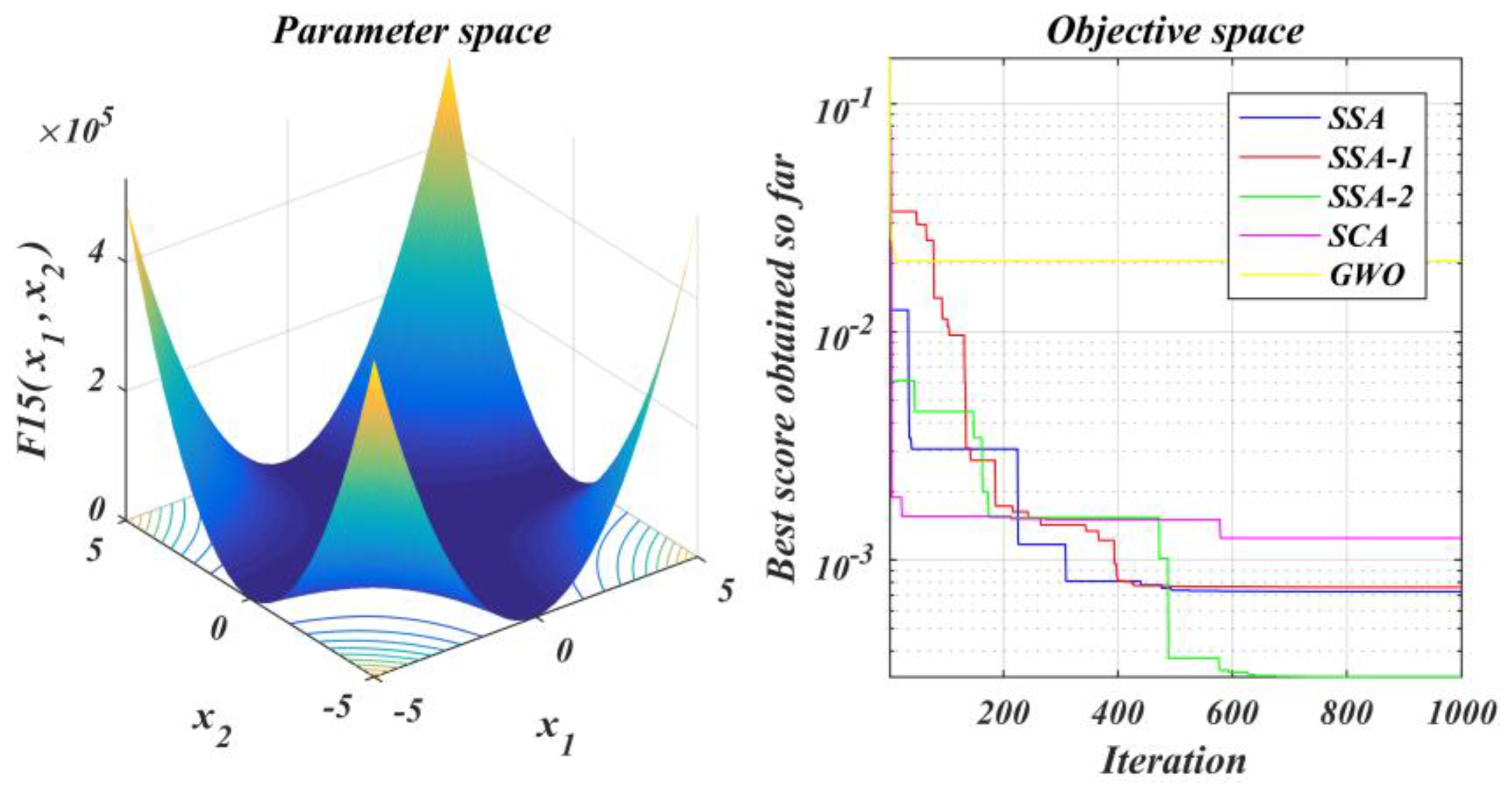
• The performance of the improved algorithm is tested under the test function set and contrasted with that of the original SSA and other methods;
• Introduction of improved salp swarm algorithm to optimize the neural network parameters and improve the predictive power of the prediction model;
• The actual tool wear data set is selected to verify its effectiveness.

In this paper, Section 2 briefly reviews the SSA algorithm and the BP neural network and its optimization. Section 3 proposes a new SSA algorithm, combines the proposed SSA2 algorithm with BP neural network to obtain the SSA2-BP prediction model, and conducts a performance comparison analysis between the improved algorithm and the original algorithm. Section 4 applies the proposed SSA2-BP algorithm to tool wear prediction, and the model prediction performance is verified by experimental comparison. Section 5 reviews the whole paper and gives recommendations for further research.

2. Related Work

2.1. The Salp Swarm Algorithm

The SSA algorithm simulates the life behavior of the salp swarm population, and the primary purpose is to randomly search an ample solution space and find the optimal solution or approximate solution. The salps population is split into two groups: leader and followers. The location of salps is defined in an n-dimensional search space, where n is the number of variables for a given problem [17]. In the salp swarm algorithm, the initial population is randomly generated. The search space is set as N × n dimension. The algorithm generates the initial population through the following formula, described mathematically in Equation (1).

$$X_{N\times n}=rand(N\times n)\times (ub-lb)+lb$$

(1)

Among them, ub and lb are abbreviations that stand for the upper and lower limits, respectively.

The leader changes with the location of the food source, updated according to Equation (2).

$$x_j^i=\left\{\begin{array}{cc}{F}_j+c_1[(u{b}_j-l{b}_j)c_2+l{b}_j],& c_3\ge 0\\ F_j-c_1[(u{b}_j-l{b}_j)c_2+l{b}_j],& c_3<0\end{array}\right.$$

(2)

Among them, $x_j^1$ represents the leader’s position, F_j represents the food-source’s location, and c₂ and c₃ are both random on [0,1]. C₂ determines the leader’s moving speed, c₃ determines the positive and negative direction of the leader’s movement, and the parameter c₁ is the time variable coefficient. The c₁ is obtained by Equation (3).

$$c_1=2e^{-{(4t/T_{max})}^2}$$

(3)

where t represents the iteration number, and T_max represents the set maximum that has been specified.

The position of the follower is updated based on the position of the leader, with consideration for the position of the preceding person. Using Newton’s law of motion equation, the followers are updated according to Equation (4).

$$x_j^i=\frac{(x_j^i+x_j^{i-1})}{2}$$

(4)

where $x_j^i$ denotes the follower’s location and $x_j^{i-1}$ represents the position of the previous follower.

2.2. BP Algorithm and Optimization

The back propagation neural network is a traditional neural network solved using the BP algorithm. It is trained by using samples, and it continuously adjusts the network’s weights and thresholds to move closer to the desired output. It is a widely used neural network model, mostly used for function approximation, model identification and classification, and time series prediction.

The BP network consists of input, implicit, and output layers. The network usually uses Sigmoid differentiable functions and linear functions as the excitation functions of the network, and continuously adjusts the network weights and thresholds by back-propagating the error function so that the error function is minimal.

The BP neural network has good self-learning, self-adaptive, nonlinear approximation, and other capabilities, but the BP neural network uses the gradient descent method, which is essentially a single-point search algorithm, there are some inherent defects, which can easily generate local extreme points, and the convergence speed is slow. In response to the above problems, researchers have proposed many optimization schemes for the BP neural network. Considering that the salp algorithm can easily solve nonlinear problems and other characteristics, this paper uses the improved salp algorithm to optimize the BP network. The BP network is optimized using an improved bottle sheath algorithm to find a better search space and then search for the optimal solution in a smaller search space.

3. Improved Algorithm and Its Combination with BP

The neural network has a significant data fitting and prediction ability, but it is greatly affected by the initial weight threshold. A metaheuristic algorithm is utilized to optimize the model hyperparameters and further raise the model prediction capability. For the inherent defects of the meta-heuristic algorithm itself, primarily, the SSA algorithm is improved by using chaotic mapping and an attenuation factor. Moreover, the improved SSA algorithm is used to solve the optimal weights and thresholds for the BP, hence enhancing the accuracy of model prediction. Ultimately, the real data on knife abrasion durability are utilized to complete the prediction. In order to ascertain whether or not the revised algorithm is successful, a benchmark function is selected for the purpose of evaluating the functionality of the algorithm. The improved algorithm outperformed the comparative approach in experiments. Figure 1 depicts the paper’s overall idea structure.

3.1. Introducing the Improved Algorithm of Chaotic Mapping

The population initialization of traditional SSA is mainly generated in a random manner [34], which makes the randomly generated initial population not evenly distributed in the entire search space. To obtain an initial value population that is more conducive to optimization before the algorithm iteration, and further improve the performance of the algorithm, many studies have applied chaos theory to population initialization [35]. E. Varol Altay et al. [36] integrated chaos into the Bird Swarm Algorithm (BSA) to improve the global convergence feature by stopping the local search scheme from becoming convergent too soon. Six different chaotic league championship algorithms were proposed and explained in detail by H. Bingol et al. [37]. Chaos theory is recognized as very useful in many engineering applications [38]. It is one of the most prevalent mathematical methods used to maximize the efficiency of metaheuristic algorithms in past years.

The main idea of the chaotic sequence is to generate a chaotic sequence through mapping the relationship between the interval [0,1] and convert it into the search space of the population. There are many ways to generate chaotic sequences. The uniformity of the sequence generated by Tent mapping is better [34]. Its mathematical expression is as follows: i = 1, 2, …, N is the population number, j = 1, 2, 3, …, n is the sequence number of the chaotic variable, μ is the chaotic coefficient, the value range is (0,2], and μ = 2 is selected in this paper.

$$y_{j+1}^i=\left\{\begin{array}{cc}\mu y_j^i,& y_j^i<0.5\\ \mu (1-y_j^i),& y_j^i\ge 0.5\end{array}\right.$$

(5)

By formula (5), n chaotic sequences can be obtained, and the obtained chaotic sequences are inversely mapped into the search space to obtain individual position vectors. Therefore, the improved population initialization is shown in Equation (6).

$$x_j^i=y_j^i\times (u{b}_i-l{b}_i)+l{b}_i$$

(6)

3.2. Introduce the Attenuation Factor to Update the Follower Position

In the SSA, the leader conducts a global search by following the leader of a food-source. The follower completes the local development process of the algorithm with the leader’s guidance. It can be seen from the above formula (4) that when the leader enters the local optimum, the update mechanism of the followers is not easy to make the algorithm leave the local optimum, resulting in premature convergence [33].

To solve the above problems, a decay factor λ is introduced into the follower update formula, so that the population individuals can fully move and search in the space in the global search stage during the preglobal search phase, and at the same time, to enable the algorithm to perform a more accurate search in the local search phase at the later stage to improve algorithm performance.

The decay factor λ is a nonlinear decreasing function that decreases with iteration. It is introduced into the follower’s positional renewal method and λ is defined as Equation (7).

$$\lambda =e^{-a(\frac{t}{T_{\max }})}$$

(7)

The formula of the attenuation factor is derived from Equation (3), wherein the parameter a is determined to be 15 through experiments. Then the follower update after the introduction of the decay factor λ is shown in Equation (8).

$$x_j^i=\frac{\lambda }{2}(x_j^i+x_j^{i-1})$$

(8)

In this way, the follower can generate adaptive updates with iteration, thereby improving the solving speed of the algorithm and reducing the phenomena of early convergence in the SSA. At the same time, such an improvement is also conducive to reducing the prediction error and improving the tool prediction model’s accuracy.

The improved population initialization algorithm mentioned in this paper is recorded as SSA1, and the algorithm with chaotic map and decay factor added in this paper is recorded as SSA2. The pseudocode of the SSA2 is (Algorithm 1):

Algorithm 1: Improved Salp Swarm Algorithm (SSA2)
(1)	generate initial population xi (i = 1, …, N) based on Tent mapping
(2)	while t < Tmax
(3)	calculate the fitness value
(4)	update c1 according to Equation (3)
(5)	for each individual xi
(6)	if (i < N/2)
(7)	update the leader position by Equation (2)
(8)	else
(9)	Update the decay factor λ by Equation (7)
(10)	Update the follower position by Equation (8)
(11)	end
(12)	end
(13)	correct individual positions accordance with the upper and lower bounds
(14)	end
(15)	Return the optimal individual fitness value and position

3.3. SSA2-BP Model

The BP network hyperparameters were refined using the improved salps algorithm (SSA2), and the SSA2-BP prediction method was constructed to complete tool wear life prediction. In the initial stage, the salps algorithm randomly generates a set of initial populations. In the hyperparameter problem of optimizing the BP neural network, the initial population solves the optimal position through iteration, that is, the optimal solution of neural network weights and thresholds. The SSA2-BP algorithm flow is shown in Figure 2.

3.4. Performance Analysis of the SSA2 Algorithm

The first 15 benchmark functions in the literature [17] were selected to test the performance, including single-peak, multi-peak, and compound functions. The relevant properties of the functions are shown in

Table 1. Unimodal benchmark functions.

Functions	Dim	Space	Optimum
$F_1(x)={\displaystyle \sum _{i=1}^n{x}_i^2}$	20	[−100,100]	0
$F_2(x)={\displaystyle \sum _{i=1}^n\left|x_i\right|}+{\displaystyle \prod _{i=1}^n\left|x_i\right|}$	20	[−10,10]	0
$F_3(x)={\displaystyle \sum _{i=1}^n({\displaystyle \sum _{j=1}^i{x}_j}}{)}^2$	20	[−100,100]	0
$F_4(x)=\mathit{max}\{\begin{array}{cc}\left|x_j\right|,& 1\le i\le n\}\end{array}$	20	[−100,100]	0
$F_5(x)={\displaystyle \sum _{i=1}^{n-1}[100(x_{i+1}-x_i^2}{)}^2+{(x_i-1)}^2]$	20	[−30,30]	0
$F_6(x)={\displaystyle \sum _{i=1}^n{([x_i+0.5])}^2}$	20	[−100,100]	0
$F_7(x)={\displaystyle \sum _{i=1}^{n}i{x}_i^4}+random[0,1)$	20	[−1.28,1.28]	0

,

Table 2. Multimodal benchmark functions.

Functions	Dim	Space	Optimum
$F_8(x)=\underset{i=1}{\overset{n}{\Sigma }}-x_{i}sin(\sqrt{\left|x_i\right|})$	20	[−500,500]	−418.98 × 5
$F_9(x)={\displaystyle \sum _{i=1}^n[x_i^2}-10cos(2\pi x_i)+10]$	20	[−5.12,5.12]	0
$F_{10}(x)=-20exp\left(-0.2\sqrt{\frac{1}{n}{\displaystyle \sum _{i=1}^n{x}_i^2}}\right)-exp\left(\frac{1}{n}{\displaystyle \sum _{i=1}^{n}cos(2\pi x_i)}\right)+20+e$	20	[−32,32]	0
$F_{11}(x)=\frac{1}{4000}{\displaystyle \sum _{i=1}^n{x}_i^2}-{\displaystyle \prod _{i=1}^{n}cos(\frac{x_i}{\sqrt{i}}})+1$	20	[−600,600]	0
$F_{12}(x)=\frac{\pi }{n}\left\{10sin(\pi y_1)+{\displaystyle \sum _{i=1}^{n-1}{(y_i-1)}^2[1+10{sin}^2(\pi y_{i+1})]+{(y_n-1)}^2}\right\}+\underset{i=1}{\overset{n}{\Sigma }}u(x_i,10,100,4)$ $y_i=1+\frac{x_i+1}{4}$ $u(x_i,a,k,m)=\left\{\begin{array}{c}k{(x_i-a)}^m{x}_i>a\\ 0-a<x_i<a\\ k{(-x_i-a)}^m{x}_i<-a\end{array}\right.$	20	[−50,50]	0
$\begin{array}{l}{F}_{13}(x)=0.1\left\{{sin}^2(3\pi x_1)+{\displaystyle \sum _{i=1}^n{(x_i-1)}^2[1+{sin}^2(3\pi x_i+1)]}\right.\\ \left.+{(x_n-1)}^2[1+{sin}^2(2\pi x_n)]\right\}+{\displaystyle \sum _{i=1}^{n}u(x_i,5100,4)}\end{array}$	20	[−50,50]	0

and

Table 3. Composite benchmark functions.

Functions	Dim	Space	Optimum
$\begin{array}{l}{F}_{14}(CF1):\\ f_1{f}_2{f}_3,\dots ,f_{10}=SphereFunction\\ [{\sigma }_1,{\sigma }_2,{\sigma }_3,\dots ,{\sigma }_{10}]=[1,1,1,\dots 1]\\ [{\lambda }_1,{\lambda }_2,{\lambda }_3,\dots ,{\lambda }_{10}]=[5/100,5/100,5/100,\dots 5/100]\end{array}$	10	[−5,5]	0
$\begin{array}{l}{F}_{15}(CF2):\\ f_1{f}_2{f}_3,\dots ,f_{10}=Griewank’sFunction\\ [{\sigma }_1,{\sigma }_2,{\sigma }_3,\dots ,{\sigma }_{10}]=[1,1,1,\dots 1]\\ [{\lambda }_1,{\lambda }_2,{\lambda }_3,\dots ,{\lambda }_{10}]=[5/100,5/100,5/100,\dots 5/100]\end{array}$	10	[−5,5]	0

, which specify the information of the elements, such as expression, search space, dimension, and the theoretical optimal value of the function.

Among them, F1~F7 are unimodal functions to test the exploitation ability, F8~F13 are multimodal functions to test the searchability of an algorithm, and F14 and F15 are compound functions to test the stability of the algorithm.

3.4.1. Parameter Setting and Experimental Environment

The simulation experiment execution environment was Intel(R) Core (TM) i5-8250U CPU @ 1.60 GHz 1.80 GHz, memory 8 GB, Windows 64-bit operating system, and Matlab2016b was used to debug and run the algorithm. The N was fixed to 30, while the maximum number of iterations was chosen to be 1000. SSA, SSA1, and Sine Cosine Algorithm (SCA) in the literature [39] and Grey Wolf Algorithm (GWO) in the literature [40] were selected for comparison to measure the performance of the enhanced algorithm.

3.4.2. Benchmark Function Test Results

To eliminate the randomness of the algorithm calculation, each algorithm was independently run 30 times on the test function set, and the average (AVG) and standard deviation (STD) of the results of the algorithm to solve the test function were recorded. The two datasets reflected the solution accuracy and solution stability of the algorithm, respectively.

Table 4. Benchmark function test results.

Functions	Results	SSA	GWO	SCA	SSA1	SSA2
F1	AVG	1.29 × 10−8	2.96 × 10−59	0.0534	1.24 × 10−8	1.85 × 10−213
	STD	3.64 × 10−9	5.64 × 10−59	0.1465	3.01 × 10−9	0
F2	AVG	0.0033	8.68 × 10−67	1.20 × 10−18	1.18 × 10−5	6.28 × 10−108
	STD	0.0156	1.97 × 10−66	4.66 × 10−18	2.33 × 10−5	1.16 × 10−108
F3	AVG	1.83 × 10−9	3.27 × 10−54	5.62 × 10−10	1.65 × 10−9	1.78 × 10−213
	STD	8.19 × 10−10	1.13 × 10−53	2.03 × 10−9	6.69 × 10−10	0
F4	AVG	1.49 × 10−5	8.36 × 10−37	1.15 × 10−7	1.58 × 10−5	1.18 × 10−107
	STD	3.46 × 10−6	1.64 × 10−36	4.71 × 10−7	2.92 × 10−6	1.08 × 10−108
F5	AVG	40.1246	6.1361	7.2296	33.5711	1.18 × 10−107
	STD	78.1914	0.6773	0.4218	69.6541	1.08 × 10−108
F6	AVG	5.69 × 10−10	9.95 × 10−7	0.4356	6.37 × 10−10	7.44 × 10−10
	STD	5.69 × 10−10	9.95 × 10−7	0.4354	6.37 × 10−10	7.44 × 10−10
F7	AVG	0.0073	0.0002	0.0025	0.0057	4.39 × 10−5
	STD	0.0045	0.0001	0.0028	0.0033	4.06 × 10−5
F8	AVG	−2672.0626	−2770.75	−2235.67	−2818.94	−2737.62
	STD	324.5513	311.40	106.34	343.12	381.754
F9	AVG	20.2425	0.4824	0	0	0
	STD	9.8763	1.5053	0	0	0
F10	AVG	1.1823	4.97 × 10−15	4.14 × 10−14	0.5673	8.88 × 10−16
	STD	1.0645	1.30 × 10−15	1.24 × 10−13	0.8484	0
F11	AVG	0.2006	0.0155	0.0218	0.2587	0
	STD	0.1106	0.0164	0.0595	0.1515	0
F12	AVG	0.2964	0.0023	0.0864	0.3066	1.54 × 10−11
	STD	0.5752	0.0076	0.0364	0.738	5.22 × 10−12
F13	AVG	0.0025	0.0354	0.2818	0.0005	7.33 × 10−11
	STD	0.0055	0.0592	0.0915	0.002	3.79 × 10−11
F14	AVG	0.9986	4.8623	1.2955	0.9981	0.9982
	STD	0	4.4948	0.7265	0	0
F15	AVG	0.0007	0.0049	0.0009	0.0007	0.0004
	STD	0.0001	0.0084	0.0004	0.0002	0.0002

provides the statistical findings.

As seen above, in the unimodal function, the SSA2 algorithm in this paper obtained six optimal solutions except for F6, and SSA obtained the optimal solution for F6. In the multimodal function, the SSA2 algorithm found the optimal solutions on F9, F10, F11, F12, and F13, especially on F11 and F12. In the composite function, SSA1 found the optimal value on F14, SSA2 found the optimal value on F15, while the SSA2 algorithm obtained smaller variance values. Therefore, the SSA2 algorithm had a better solution accuracy than SSA, SCA, and GWO because the SSA2 algorithm introduced the decay factor and chaotic mapping, which allowed the algorithm to avoid falling into local convergence and improved the convergence speed. It can be seen that the improvement strategy improved the development ability of the algorithm and showed that the improvement of the algorithm had a certain effectiveness. Meanwhile, in the experiment of the benchmark function, the variance of the SSA2 algorithm test results was smaller, which indicates that the improved algorithm had a better stability.

3.4.3. Convergence Analysis

The convergence curves of the algorithm on the function test are shown in Figure 3, Figure 4, Figure 5, Figure 6, Figure 7 and Figure 8 below, which are the partial convergence results curves of the algorithm on the unimodal function, the multimodal function, and the composite function.

As seen from the above figure, on the unimodal function, the SSA2 algorithm had a significantly better convergence speed and solution accuracy, especially in F7; the SSA2 algorithm found a solution closer to the theoretical optimal value and could quickly converge. In the multimodal function, the SSA2 algorithm had a better convergence speed. For example, in F13, the algorithm initially fell into the local extremum, but the later algorithm also jumped out of the optimal local value with the iteration. In the composite function, the SSA2 algorithm could trip out the top local optimality many times and could achieve better solution accuracy. Especially on F15, SSA2 had a better accuracy of solution compared with the original SSA algorithm.

3.4.4. Rank Sum Test

Comparing algorithms using mean and standard deviation is insufficient. To show that a new algorithm is significantly better than existing ones, a statistical test should be conducted [41]. To test the variability between algorithms, statistical tests were performed. The Wilcoxon rank-sum test reflected the algorithm differences. When the p-value is less than 0.05, the new approach outperformed. For further proof of the validity of the SSA2 proposed in this paper, a Wilcoxon rank-sum test was performed, where h was 1, which meant there was a large difference, and h was 0, which meant no significant difference.

The improved algorithm (SSA2) and SSA1, the original SSA algorithm, the SCA algorithm, and the GWO algorithm, respectively, were subjected to the rank sum test, and the results were recorded in

Table 5. Rank sum test.

Algorithm	p-Value	h
SSA2vs.SSA1	0.110	0
SSA2vs.SSA	0.017	1
SSA2vs.SCA	0.198	0
SSA2vs.GWO	0.262	0

.

The statistical test findings revealed that in the rank sum test for SSA2 and SSA, the value of p-value was less than 0.05, indicating that the SSA2 proposed was substantially different from the original algorithm, and SSA2 was found to be more effective than the SSA algorithm, which validated the effectiveness of the improved strategy proposed.

3.4.5. Time Complexity Analysis

In addition to the rank-sum test, convergence curve, etc., the time complexity analysis of the SSA2 was also carried out. The dimension is n, assuming N is the population size of the algorithm, the time for setting parameters is t₁, the time for generating random numbers is t₂, the time for solving fitness is f(n), the time for sorting fitness is t₃, and the time to generate c₁, c₂, c₃ is t₄, and the time for the individual population to update each dimension is t₅, then the population initialization time of the SSA algorithm is shown in Equation (9).

$${\mathrm{T}}_1=\mathrm{O}\{t_1+N[t_{2}n+f(n)+t_3]\}=O[n+f(n)]$$

(9)

The time complexity of the follower position update phase is shown in Equation (10).

$$T_2=O[t_4+\frac{N}{2}(2t_1+t_5)n]=O(n)$$

(10)

In the improved SSA algorithm, the chaotic mapping time is set as t₅, the generation time of the decay factor as t₆, and the initialization time of the SSA2 algorithm is shown in Equation (11).

$${\mathrm{T}}_1=\mathrm{O}\{t_1+N[t_{5}n+f(n)+t_3]\}=O[n+f(n)]$$

(11)

The time complexity of the follower position update phase is shown in Equation (12).

$$T_2=O[t_6+\frac{N}{2}(2t_1+t_5)n]=O(n)$$

(12)

To sum up, the improved SSA algorithm did not change the time complexity of the original algorithm and did not reduce the execution efficiency of the algorithm.

4. Tool Wear Prediction Application

The metaheuristic algorithm is capable of solving global solutions in a multidimensional search space and is widely used in the training of neural networks. Therefore, we optimized the network using the proposed improved SSA algorithm to accomplish tool wear prediction.

The 2010 American PHM Association public tool wear data set was selected, and the c1, c4, and c6 data were combined with a sample size of 945. The data contained eight items (x, y, and z-axis cutting forces, acoustic emission signals, x, y, and z-axis vibration, and tool wear). The data were divided using the hold-out method, with 80% used for training and 20% for testing.

4.1. Data Preprocessing

The original data’s cutting force, vibration, and acoustic emission signal were periodic high-frequency signals. The actual data were processed using the time-domain-frequency-domain feature extraction method. The root means square values of the time domain features of the cutting force and vibration signals, X_rms, were selected. The Fourier transform was used to convert the acoustic emission signals into frequency domain signals, which were normalized and then used as feature inputs. The formula for the root-mean-square values of the time-domain features is shown in Equation (13).

$$X_{rms}=\sqrt{\frac{1}{N}{\displaystyle \sum _{i=1}^N{X}_i}}$$

(13)

N symbolizes the total number of signals, whereas X_i represents signal points. The acoustic emission signal data points were divided into odd and even groups, and Fourier transforms using Equations (14) and (15) were selected as inputs, respectively, with the following expressions.

$$X(K)=X_1(k)+W_M^k{X}_2(k)$$

(14)

$$X(K+\frac{N}{2})=X_1(k)+W_M^k{X}_2(k)$$

(15)

where $W_M^k$ is the rotation factor, which is obtained from the following equation.

$$W_M^{mk}=e^{-j\frac{2\pi }{M}mk},M=0,1,\dots ,M-1$$

(16)

4.2. Model Network Structure Design

This paper used a multi-input single-output BP network containing one hidden layer to build a prediction model. The indicators of each data set were taken as the input, and the tool wear was taken as the output. The model had seven input nodes and one output node. The hidden layer’s neuron depends on the actual problem’s sophistication and anticipated error threshold. During network design, the hidden layer neuron count must be determined. In this study, the empirical formula determined the hidden layer’s neuron range, and then experience and various tests decided its neuron count. The empirical formula is given in Equation (17).

$$x=\sqrt{a+b}+i$$

(17)

where a and b represent the neuron numbers of input and output layers, respectively, and i is a positive integer from 1 to 10.

An experimental comparison determined the ideal number of hidden-layer nodes in the range of hidden-layer neurons, as shown in the

Table 6. Results of experiments to determine the number of nodes.

Num	3	4	5	6	7	8	9	10	11	12
error	0.03068	0.1026	0.04248	0.05256	0.03429	0.03235	0.03769	0.03383	0.03965	0.02708

below, where Num is the number of hidden-layer’s neurons and Error means the training set mean squared error.

Therefore, twelve neurons were selected for the hidden layer in this experiment.

4.3. Selection of the Excitation Function and Fitness Function

The network usually adopts Sigmoid differentiable function and linear function as the excitation function, and the S-type tangent function was selected as the excitation function in this paper. The formula is given in Equation (18).

$$f(x)=\frac{1}{1+e^{-x}}$$

(18)

The fitness function, also known as the objective function, was set to the mean square error of the predicted and true values of the training data in the model training. The formula is as follows. y denotes the true value and $\widehat{y}$ denotes the predicted value.

$$f=\sqrt{\frac{1}{n}{\displaystyle \sum _{i=1}^n{\left(y-\widehat{y}\right)}^2}}$$

(19)

Considering the decision variables as the weights and thresholds of the neural network, the range of taken values was restricted to [−1.5,1.5], which was the constraint. When the taken value exceeded the bound, the corresponding boundary value was taken instead of the value.

4.4. Model Evaluation Indicators

For model quality, the following three commonly used parameters were applied for assessment, including MAE, MSE, RMSE, and R² (coefficient of determination) with the following equations.

$$MAE=\frac{1}{n}{\displaystyle \sum _{i=1}^n|}{\widehat{y}}_i-y_i|$$

(20)

$$MSE=\frac{1}{n}{\displaystyle \sum _{i=1}^n({\widehat{y}}_i-y_i{)}^2}$$

(21)

$$RMSE=\sqrt{\frac{1}{n}{\displaystyle \sum _{i=1}^n{\left({\widehat{y}}_i-y_i\right)}^2}}$$

(22)

$$R^2=1-\frac{{\displaystyle {\sum }_i{\left({\widehat{y}}_i-y_i\right)}^2}}{{\displaystyle {\sum }_i{\left(y_i-\overline{y}\right)}^2}}$$

(23)

$$\overline{y}=\frac{1}{n}{\displaystyle \sum _{i=1}^n{y}_i}$$

(24)

where $y_i$ is the true value, ${\widehat{y}}_i$ indicates the predicted value. The smaller the error, the more accurate the model prediction. The R² measured how well the predicted value fits the true value, and the value ranged from 0 to 1. The closer R² is to 1, the better the model’s prediction.

4.5. Experimental Results

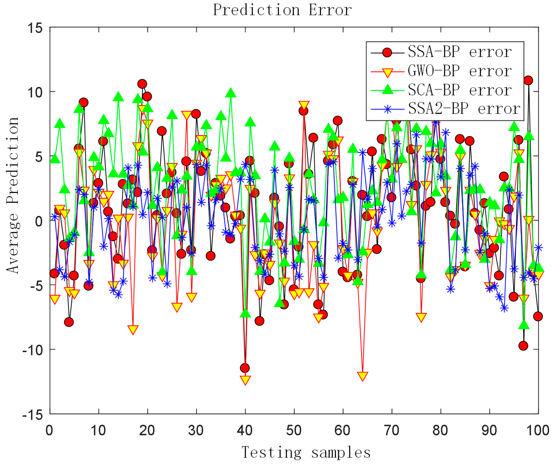
The combination algorithm of SCA and BP (SCA-BP), the combination algorithm of GWO and BP (GWO-BP), the SSA-BP algorithm, and the SSA2-BP algorithm were compared and analyzed. Some sample data were selected and the predictions of the four prediction models’ Values, the true value comparison chart (Figure 9), and the prediction error chart were drawn (Figure 10).

The prediction error values of the algorithm-optimized prediction model were recorded, and to avoid chance, they were run several times and averaged. The results are shown in

Table 7. Prediction error values.

Indicators	SCA-BP	GWO-BP	SSA-BP	SSA2-BP
MAE	4.96	3.94	4.91	2.32
MSE	40.2	32.05	34.4	9.36
RMSE	6.34	5.66	5.87	3.06
R2	0.955	0.964	0.962	0.989

.

From the above graphs, it can be seen that the SSA2-BP prediction model had higher R² values and smaller prediction error values compared to the other algorithms in the graphs. Compared with the original algorithm model SSA-BP, the R² value of the SSA2-BP model improved from 0.962 to 0.989, and the MSE value was reduced from 34.4 to 9.36, which is a 72% improvement compared to the original algorithm. This was due to the addition of chaotic mapping and decay factor to the algorithm, which gave SSA2 better solution accuracy compared with other algorithms, which made the SSA2-BP model have a better prediction ability and further proved the algorithm enhancement technique is feasible and successful.

5. Conclusions

This research provided a tool wear life prediction approach using chaotic mapping salp swarm. To address the model’s shortcomings, firstly, chaotic mapping and decay factor were introduced to improve the salp swarm algorithm, improve the BP network’s convergence speed and other flaws using the updated algorithm., and then improve the prediction ability of the prediction model.

The experimental findings revealed that the improved algorithm SSA2 had a higher solution accuracy and could leave the local optimum several times and converge rapidly compared with other metaheuristic algorithms. In addition, in applying tool wear prediction, the SSA2-BP model achieved higher R² values and smaller prediction error values. Compared with the original algorithm model SSA-BP, the R² value of the SSA2-BP model improved from 0.962 to 0.989, and the MSE value was reduced from 34.4 to 9.36, which is a 72% improvement compared with the original algorithm. In other words, the improved algorithm proposed in this paper had a better solution accuracy than other algorithms.

However, the improved algorithm still has shortcomings. The effectiveness of SSA2 may decrease significantly with the increase in variables due to the fast convergence rate and stimulation of development toward local optimal solutions when solving difficult optimization problems with many alternatives and local solutions. Meanwhile, the neural network model is greatly affected by the amount of training data and other parameters, and further research on the robustness of the algorithm and the accuracy and generalization of the model is needed in subsequent studies to further improve the model prediction accuracy.

In addition, some novel metaheuristic algorithms can also be used to solve the prediction problem of deep learning models, and in the next work, combining these new algorithms and extending this type of optimization problem need to be considered. Meanwhile, some representative new multi-objective optimization algorithms can be used to solve complex multi-objective optimization problems, and research related to multi-objective optimization algorithms is also necessary in the next work.

References

1. Sick, B. On-line and indirect tool wear monitoring in turning with artificial neural networks: A review of more than a decade of research. Mech. Syst. Signal Process. 2002, 16, 487–546. [Google Scholar] [CrossRef]
2. Kilic, K.; Toriya, H.; Kosugi, Y.; Adachi, T.; Kawamura, Y. One-Dimensional Convolutional Neural Network for Pipe Jacking EPB TBM Cutter Wear Prediction. Appl. Sci. 2022, 12, 2410. [Google Scholar] [CrossRef]
3. Wang, G.; Li, Q.; Wang, L.; Zhang, Y.; Liu, Z. Elderly fall detection with an accelerometer using lightweight neural networks. Electronics 2019, 8, 1354. [Google Scholar] [CrossRef]
4. Zhang, J.; Zeng, Y.; Starly, B. Recurrent neural networks with long term temporal dependencies in machine tool wear diagnosis and prognosis. SN Appl. Sci. 2021, 3, 1–13. [Google Scholar] [CrossRef]
5. Lee, W.K.; Abdullah, M.D.; Ong, P.; Abdullah, H.; Teo, W.K. Prediction of flank wear and surface roughness by recurrent neural network in turning process. J. Adv. Manuf. Technol. 2021, 15, 1. [Google Scholar]
6. Wang, J.; Yan, J.; Li, C.; Gao, R.X.; Zhao, R. Deep heterogeneous GRU model for predictive analytics in smart manufacturing: Application to tool wear prediction. Comput. Ind. 2019, 111, 1–14. [Google Scholar] [CrossRef]
7. Yu, J.; Liang, S.; Tang, D.; Liu, H. A weighted hidden Markov model approach for continuous-state tool wear monitoring and tool life prediction. Int. J. Adv. Manuf. Technol. 2017, 91, 201–211. [Google Scholar] [CrossRef]
8. Lin, M.; Wanqing, S.; Chen, D.; Zio, E. Evolving Connectionist System and Hidden Semi-Markov Model for Learning-Based Tool Wear Monitoring and Remaining Useful Life Prediction. IEEE Access 2022, 10, 82469–82482. [Google Scholar] [CrossRef]
9. Duan, J.; Zhang, X.; Shi, T. A Hybrid Attention-Based Paralleled Deep Learning Model for Tool Wear Prediction. Expert Syst. Appl. 2023, 211, 118548. [Google Scholar] [CrossRef]
10. He, Z.; Shi, T.; Xuan, J.; Li, T. Research on tool wear prediction based on temperature signals and deep learning. Wear 2021, 478, 203902. [Google Scholar] [CrossRef]
11. Alonso, F.J.; Del Castillo, J.M.; Pintado, P. Application of singular spectrum analysis to the smoothing of raw kinematic signals. J. Biomech. 2005, 38, 1085–1092. [Google Scholar] [CrossRef] [PubMed]
12. Akyol, S.; Alatas, B. Plant intelligence based metaheuristic optimization algorithms. Artif. Intell. Rev. 2017, 47, 417–462. [Google Scholar] [CrossRef]
13. Deng, W.; Liu, H.; Xu, J.; Zhao, H.; Song, Y. An improved quantum-inspired differential evolution algorithm for deep belief network. IEEE Trans. Instrum. Meas. 2020, 69, 7319–7327. [Google Scholar] [CrossRef]
14. Zhao, H.; Zhang, P.; Zhang, R.; Yao, R.; Deng, W. A novel performance trend prediction approach using ENBLS with GWO. Meas. Sci. Technol. 2022, 34, 2. [Google Scholar] [CrossRef]
15. Zhao, H.; Liu, J.; Chen, H.; Chen, J.; Li, Y.; Xu, J.; Deng, W. Intelligent diagnosis using continuous wavelet transform and gauss convolutional deep belief network. IEEE Trans. Reliab. 2022. [Google Scholar] [CrossRef]
16. Huang, C.; Zhou, X.; Ran, X.; Liu, Y.; Deng, W.; Deng, W. Co-evolutionary competitive swarm optimizer with three-phase for large-scale complex optimization problem. Inf. Sci. 2022, 619, 2–18. [Google Scholar] [CrossRef]
17. Mirjalili, S.; Gandomi, A.H.; Mirjalili, S.Z.; Saremi, S.; Faris, H.; Mirjalili, S.M. Salp Swarm Algorithm: A bio-inspired optimizer for engineering design problems. Adv. Eng. Softw. 2017, 114, 163–191. [Google Scholar] [CrossRef]
18. Bhandari, A.K.; Kandhway, P.; Maurya, S. An efficient binary salp swarm algorithm with crossover scheme for feature selection problems. Knowl.-Based Syst. 2018, 154, 43–67. [Google Scholar]
19. Bhandari, A.K.; Kandhway, P.; Maurya, S. Salp swarm algorithm-based optimally weighted histogram framework for image enhancement. IEEE Trans. Instrum. Meas. 2020, 69, 6807–6815. [Google Scholar] [CrossRef]
20. Hoang, N.D.; Huynh, T.C.; Tran, X.L.; Tran, V.D. A Novel Approach for Detection of Pavement Crack and Sealed Crack Using Image Processing and Salp Swarm Algorithm Optimized Machine Learning. Adv. Civ. Eng. 2022, 2022. [Google Scholar] [CrossRef]
21. Nejad, M.B.; Shiri, M.E. A new enhanced learning approach to automatic image classification based on Salp Swarm Algorithm. Comput. Syst. Sci. Eng. 2019, 34, 91–100. [Google Scholar] [CrossRef]
22. Salgotra, R.; Singh, U.; Singh, S.; Singh, G.; Mittal, N. Self-adaptive salp swarm algorithm for engineering optimization problems. Appl. Math. Model. 2021, 89, 188–207. [Google Scholar] [CrossRef]
23. Duan, Q.; Wang, L.; Kang, H.; Shen, Y.; Sun, X.; Chen, Q. Improved Salp Swarm Algorithm with Simulated Annealing for Solving Engineering Optimization Problems. Symmetry 2021, 13, 1092. [Google Scholar] [CrossRef]
24. Zhang, H.; Cai, Z.; Ye, X.; Wang, M.; Kuang, F.; Chen, H.; Li, C.; Li, Y. A multi-strategy enhanced salp swarm algorithm for global optimization. Eng. Comput. 2020, 38, 1177–1203. [Google Scholar] [CrossRef]
25. Abualigah, L.; Shehab, M.; Alshinwan, M.; Alabool, H. Salp swarm algorithm: A comprehensive survey. Neural Comput. Appl. 2020, 32, 11195–11215. [Google Scholar] [CrossRef]
26. Bairathi, D.; Gopalani, D. Numerical optimization and feed-forward neural networks training using an improved optimization algorithm: Multiple leader salp swarm algorithm. Evol. Intell. 2021, 14, 1233–1249. [Google Scholar] [CrossRef]
27. Kassaymeh, S.; Al-Laham, M.; Al-Betar, M.A.; Alweshah, M.; Abdullah, S.; Makhadmeh, S.N. Backpropagation Neural Network optimization and software defect estimation modelling using a hybrid Salp Swarm optimizer-based Simulated Annealing Algorithm. Knowl.-Based Syst. 2022, 244, 108511. [Google Scholar] [CrossRef]
28. Pan, J.S.; Shan, J.; Zheng, S.G.; Chu, S.C.; Chang, C.K. Wind power prediction based on neural network with optimization of adaptive multi-group salp swarm algorithm. Clust. Comput. 2021, 24, 2083–2098. [Google Scholar] [CrossRef]
29. Kassaymeh, S.; Abdullah, S.; Alweshah, M.; Hammouri, A.I. A hybrid salp swarm algorithm with artificial neural network model for predicting the team size required for software testing phase. In Proceedings of the 2021 International Conference on Electrical Engineering and Informatics (ICEEI), Kuala Terengganu, Malaysia, 12–13 October 2021; pp. 1–6. [Google Scholar]
30. Zivkovic, M.; Stoean, C.; Chhabra, A.; Budimirovic, N.; Petrovic, A.; Bacanin, N. Novel improved salp swarm algorithm: An application for feature selection. Sensors 2022, 22, 1711. [Google Scholar] [CrossRef]
31. Zhang, D.; Chen, Z.; Xin, Z.; Zhang, H.; Yan, W. The salp swarm algorithm based on crazy adaptation. Control Decis. 2020, 35, 2112–2120. (In Chinese) [Google Scholar]
32. Qais, M.H.; Hasanien, H.M.; Alghuwainem, S. Enhanced salp swarm algorithm: Application to variable speed wind generators. Eng. Appl. Artif. Intell. 2019, 80, 82–96. [Google Scholar] [CrossRef]
33. Fan, Q.; Chen, Z.J.; Xia, Z.H. An improved salp swarm algorithm based on refraction reverse learning mechanism and adaptive control factor. J. Harbin Inst. Technol. 2020, 52, 183–191. (In Chinese) [Google Scholar]
34. Zhou, R.; Wang, W.Q. Adaptive salps group algorithm for chaotic mapping and dynamic learning. Comput. Eng. Des. 2021, 42, 1963–1972. (In Chinese) [Google Scholar]
35. Sayed, G.I.; Hassanien, A.E.; Azar, A.T. Feature selection via a novel chaotic crow search algorithm. Neural Comput. Appl. 2019, 31, 171–188. [Google Scholar] [CrossRef]
36. Varol Altay, E.; Alatas, B. Bird swarm algorithms with chaotic mapping. Artif. Intell. Rev. 2020, 53, 1373–1414. [Google Scholar] [CrossRef]
37. Bingol, H.; Alatas, B. Chaotic league championship algorithms. Arab. J. Sci. Eng. 2016, 41, 5123–5147. [Google Scholar] [CrossRef]
38. dos Santos Coelho, L.; Mariani, V.C. Use of chaotic sequences in a biologically inspired algorithm for engineering design optimization. Expert Syst. Appl. 2008, 34, 1905–1913. [Google Scholar] [CrossRef]
39. Mirjalili, S. SCA: A sine cosine algorithm for solving optimization problems. Knowl.-Based Syst. 2016, 96, 120–133. [Google Scholar] [CrossRef]
40. Mirjalili, S.; Mirjalili, S.M.; Lewis, A. Grey wolf optimizer. Adv. Eng. Softw. 2014, 69, 46–61. [Google Scholar] [CrossRef]
41. Saremi, S.; Lewis, A.; Mirjalili, S. Biogeography-based optimization with chaos. Neural Comput. Appl. 2014, 25, 1077–1097. [Google Scholar] [CrossRef] [Green Version]
Figure 1. Overall idea frame diagram3.1. Introducing the improved algorithm of chaotic mapping.
Electronics 12 00769 g001
Figure 2. SSA2-BP neural network algorithm flow chart.
Electronics 12 00769 g002
Figure 3. F1 Convergence curve.
Electronics 12 00769 g003
Figure 4. F7 Convergence curve.
Electronics 12 00769 g004
Figure 5. F10 Convergence curve.
Electronics 12 00769 g005
Figure 6. F13 Convergence curve.
Electronics 12 00769 g006
Figure 7. F14 Convergence curve.
Electronics 12 00769 g007
Figure 8. F15 Convergence curve.
Electronics 12 00769 g008
Figure 9. Comparison of the predicted value and the true values.
Electronics 12 00769 g009
Figure 10. Error comparison chart.
Electronics 12 00769 g010