An Attention-Based Uncertainty Revising Network with Multi-Loss for Environmental Microorganism Segmentation

Abstract

The presence of environmental microorganisms is inevitable in our surroundings, and segmentation is essential for researchers to identify, understand, and utilize the microorganisms; make use of their benefits; and prevent harm. However, the segmentation of environmental microorganisms is challenging because their vague margins are almost transparent compared with those of the environment. In this study, we propose a network with an uncertainty feedback module to find ambiguous boundaries and regions and an attention module to localize the major region of the microorganism. Furthermore, we apply a mid-pred module to output low-resolution segmentation results directly from decoder blocks at each level. This module can help the encoder and decoder capture details from different scales. Finally, we use multi-loss to guide the training. Rigorous experimental evaluations on the benchmark dataset demonstrate that our method achieves higher scores than other sophisticated network models (95.63% accuracy, 89.90% Dice, 81.65% Jaccard, 94.68% recall, 0.59 ASD, 2.24 HD95, and 85.58% precision) and outperforms them.

1. Introduction

Environmental microorganisms (EMs) generally refer to living organisms found in the environment that are too small to be seen by the naked eye [1]. On the one hand, harmful microbial species are responsible for crop yield reduction, food spoilage, and even human epidemics. However, some kinds of EMs can benefit humans and can be used in medicine, the chemical industry, food processing, and many other fields. Different types of EMs have varying growth characteristics and metabolic processes and play different roles in medicine and other industries. Thus, the classification and identification of EMs are of great significance for understanding the overall picture of microorganisms and for the further development and utilization of microbial resources.

The direct visual identification of EMs is an impossible task because they have small sizes that range from 0.1 to 100 microns. To solve this issue, auxiliary equipment and technologies are often employed, with microscopy being one of the most common identification techniques [2]. However, microscope image recognition is usually performed manually and is time-consuming. Moreover, outlining EMs, that is, EM image segmentation, is also a huge challenge because they often blend in with their surroundings and have a similar visual appearance. Figure 1 shows the microscopic imaging of multiple EMs and the results of artificial segmentation. In this study, we aimed to automatically segment environmental microorganisms using microscopic imaging based on computer vision technology.

Recently, deep learning has demonstrated its advantages in multiple computer vision tasks, such as image classification and segmentation, and various deep networks have been developed to improve its performance.

An encoder–decoder structure is an important depth model for semantic image segmentation, and the research trends can be summarized as follows. The first is modifying U-Net-like structures. This type of method maintains a nearly symmetrical structure of the U-shape of the network by only adjusting each level of encoders and decoders or by adding or changing modules (such as the attention module) or predicting stages, such as TAU-Net [3] added and multiplied encoders at the deepest level. The second type is changing the symmetrical architecture to extract more information. For example, some transformer-based networks use multiple encoders but a single decoder to extract global information more precisely. Some networks even discard the structure and turn to unified update heads. The last type is enhancing the availability of models in different conditions. For example, some studies have focused on reducing the param size of networks to deploy models on integrated devices such as cameras.

The encoder–decoder depth model for semantic segmentation shows good performance in fields such as scenes; however, the following challenges in the application of EM segmentation remain. First, EMs vary significantly in size and shape, making them difficult to distinguish from their background. Second, non-ideal environments for photography and the inherent structure of EMs result in vague and blurry foreground boundaries. Moreover, the majority parts of some EMs are transparent. These parts can be easily segmented as backgrounds, and some messy backgrounds can be mispredicted as EMs. Finally, EM datasets are relatively small, with only a few hundred pictures, which makes convergence difficult, particularly for transformer-based networks.

To this end, we propose a novel network built on top of a residual feedback network [4] that has shown its effectiveness in medical image segmentation. More specifically, our model consists of two stages of the prediction process: the uncertainty feedback module to monitor segmentation failure and the attention module to capture spatial information. Furthermore, we propose a mid-pred module and refined loss function to accelerate convergence with higher segmentation accuracy. Rigorous experimental evaluations on a benchmark dataset with 21 types of EMs demonstrated that the proposed method outperforms other state-of-the-art models. In summary, our contributions are fourfold:

(1)

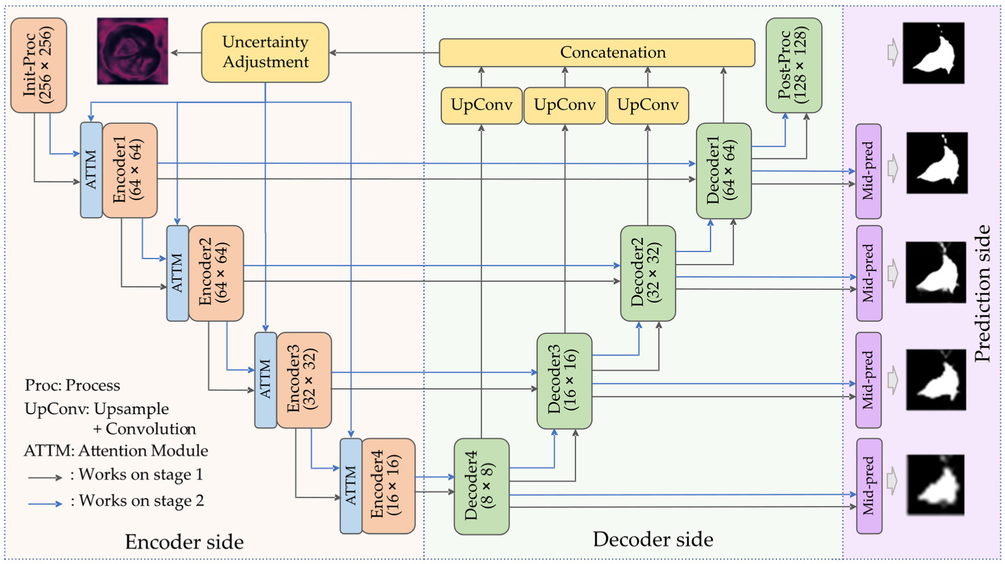
A new network structure based on an encoder–decoder architecture is proposed. The network integrates two-stage processing, uncertainty feedback, attention, and a mid-pred module, thereby enhancing the segmentation accuracy.

(2)

We created a new attention module that can effectively determine the position of EMs and capture weights from the previous encoder with an accurate perception of marginal areas.

(3)

The proposed network is integrated with the mid-pred module, which can guide the model in determining the position of the foreground area and avoid false predictions in large, confusing areas.

(4)

A new loss function was designed with mixed nominals to accelerate training.

The remaining parts of this article are organized as follows: Section 2 presents the related work. Section 3 describes the proposed network structure and computing process in detail. Section 4 presents the experimental evaluation and results. Finally, Section 5 presents the conclusions and future work.

2. Related Work

2.1. Review of Semantic Segmentation Methods in the Field of Computer Vision

In the early stages of image segmentation, an image is segmented into meaningful and non-overlapping regions corresponding to the visual perception of humans. Many classical algorithms have been developed for this task, such as the threshold-based method [5], the region growing method [6], clustering algorithms [7], the watershed algorithm [8], the graph cut method [9], the conditional random field (CRF) [10], the Markov random field (MRF) algorithms [11], and sparse feature-based algorithms [12]. The calculations in these methods are generally simple, and they depend less on the number of samples. However, these methods have many limitations in complex scenarios.

With the growth of computing abilities and large-scale annotated datasets, research on image segmentation has shifted towards pixel-level semantic segmentation, which requires the classification of each pixel based on high-level semantic information. Recently, deep learning methods have significantly improved semantic segmentation performance.

Fully convolutional networks (FCNs) [13] are among the pioneers of deep learning methods in semantic segmentation, which provide end-to-end neural networks for semantic segmentation. Subsequently, various neural networks have been proposed for semantic segmentation. U-Net [14] is one of the representative models that propose an encoder–decoder architecture based on FCN. U-Net employs deconvolution for up-sampling to increase the dimension of feature maps, and it designs jump connections between the corresponding encoding and decoding layers to preserve the low-level features of the images. U-Net and similar encoder–decoder architectures are widely used for semantic segmentation, especially for medical and satellite images. Several variants of U-Net, such as UNet++ [15], Segnet [16], MC-Unet [17], and RefineNet [18], have been developed to improve performance. The residual feedback network (RF-Net) [4] is a remarkable recent method that uses an encoder–decoder architecture such as U-Net. In addition to changing the encoder to ResNet, it also performs two-stage segmentation. Specifically, the encoder extracts information from the residual feedback module, indicating the possibility of segmentation failure. Compared with other networks, it has a higher accuracy and robustness for the segmentation of breast lesion images.

A recurrent neural network (RNN) provides another strategy to improve segmentation results, which focuses on modeling the dependencies between pixels by establishing global contextual relationships. ReNet [19] divides an image into different patches and scans them both horizontally and vertically to convert the spatial information into sequential information. Moreover, gating mechanisms such as a gated recurrent unit (GRU) and long short-term memory (LSTM) [20] have also been applied to learn image texture information and spatial model parameters and to achieve pixel-level segmentation.

Recently, transformers and their variants have also achieved significant success in the field of computer vision. The vision transformer (ViT) [21] proposed the application of a transformer from the text domain [22] to the image domain, which slices the image into 16 × 16 chunks and converts them into vectors with fixed lengths and then uses classification networks for segmentation. Since then, transformer-based models have gained popularity, such as the deformable patch-based transformer (DPT) [23], which adjusts the patch size to locate targets more accurately. With sufficient pre-training data, transformer-based networks can outperform CNN (convolutional neural network) models with fewer computations for both segmentation and target detection tasks.

In improvement strategies for different network structures in image segmentation, the attention mechanism is a widely used module that can simulate the cognitive function of individuals by selectively focusing on parts of the senses of greater importance. By reducing the information density and emphasizing certain parts, the attention module can easily capture regions of interest and enhance the accuracy by slightly increasing the size and computing complexity. Some studies, such as SA [24], MGFAN [25], CBAM [26], and coordinate attention [27], have proved the effectiveness of the attention mechanism. However, the attention mechanism must be designed for specific applications and integrated into selected networks to maximize their advantages.

In this study, we focused on the design of attention guidance, based on a residual feedback network, to improve the performance of EM segmentation. In the experiment, we compared the proposed model with different types of deep networks, such as CNNs, RNNs, and transformers, and the experimental results proved the superiority of our model.

2.2. Review of Segmentation Methods in the Field of EM Image Segmentation

Various segmentation methods have been used for EM image segmentation, which can be divided into traditional and machine-learning-based segmentation methods [28]. Traditional methods can be further divided into three categories: edge-based, threshold-based, and region-based segmentation methods [29]. However, traditional methods are often performed in an unsupervised manner and usually cannot satisfy their tasks, owing to the transparency and complexity of the microorganisms. In general, traditional methods are more suitable for small and opaque microorganisms. However, machine learning methods, such as k-means clustering and conditional random fields, have been applied in succession for these tasks. For example, Kyan et al. [30] proposed an organizing tree map network for biofilm segmentation, which pioneered the use of machine learning methods for EM segmentation.

Deep-learning methods have also gained popularity owing to improvements in computing abilities and datasets. Generally, because convolutional neural networks perform well in all types of computer vision tasks, researchers have applied CNNs to EM segmentation tasks. Kosov et al. [31] trained a DeepLab-VGG16 model to extract texture information and used CRF models to classify pixels, whereas Hung and Carpenter [32] proposed using Faster R-CNN (region with CNN features) to detect plasmodium-vivax-infected blood cells and achieved surprising accuracy. In addition, U-Net has gained popularity owing to its simple structure and surprisingly significant effects. Researchers have implemented multiple modified U-Nets for EM segmentation. MRFU-Net (multiple receptive field U-Net) changed the encoder from the FCN to the Reception module and achieved better results in EM segmentation. LCU-Net [33] changed the 3 × 3 convolution to a 1 × 3 + 3 × 1 convolution to reduce the param size and accelerate the prediction.

In addition to the aforementioned models, GANs and transformer-based networks have recently been used for EM segmentation. Aydin et al. [34] achieved a 71.72% mIoU (mean intersection over union) score in segmenting yeast cells with the help of the SegNet model, which is based on RNNs. In addition, Ang et al. [35] proposed a phase-stretch transform for segmenting floc and filamentous bacteria with better results. These studies have demonstrated the availability of new popular models for EM segmentation.

These studies achieved satisfactory results for EM image segmentation. However, most studies have focused on certain types of microorganisms; therefore, they lack versatility in dealing with various types of EMs. Furthermore, in EM segmentation tasks, the transparency of the foreground and uncertainty of the EM position may still cause mispredictions, which remains a difficult problem. As a result, though the newest networks often achieve the best results on most tasks, they might show problems when dealing with EM images. For example, although transformer-based networks perform well for many types of segmentation tasks, they require a large amount of computation before being transferred to a certain task. In contrast to large datasets, such as ADE20K [36], which has thousands of pictures, EMDS-6 [37] (which we used) has only 420 original images for segmentation. Furthermore, blurry edges and transparent insides remain challenging to the network. Therefore, there is still much scope for optimizing segmentation models. In the visual comparison in Section 4.4, we can observe the limitations of previous segmentation methods when faced with different types of EMs.

Therefore, in this study, we developed a novel method based on this motivation to overcome existing difficulties. With the proposed method, a simple and effective encoder–decoder structure can learn sufficient knowledge from a small number of data, and the new modules can accelerate the training process and improve accuracy.

3. Method

In this section, we introduce in detail the architecture of the proposed semantic segmentation network. Section 3.1 introduces our overall network architecture, and Section 3.2 describes the uncertainty revising network. The mid-pred module is described in Section 3.3. The attention module is described in Section 3.4. Finally, the proposed multi-loss function is introduced in Section 3.5.

3.1. Network Architecture

Figure 2 shows the overall architecture of our end-to-end network for microorganism segmentation. The proposed network is formed as an encoder–decoder structure that includes two stages. In the first stage, we used the U-Net-like structure to make a rough prediction from the input. Before the next stage, the uncertainty feedback module was employed to extract feedback from the decoders to calculate the estimated error rate in the rough prediction result. In the second stage of inference, although the same structure was applied, the uncertainty feedback was considered. To combine the encoded data and uncertainty feedback, and to enhance the performance of the segmentation result, we used an attention module to emphasize regions of interest and attach data from feedback to encoders. In addition, during the two stages of inference, mid-pred modules directly generated low-resolution outputs from the decoder blocks, which also affects the network optimization.

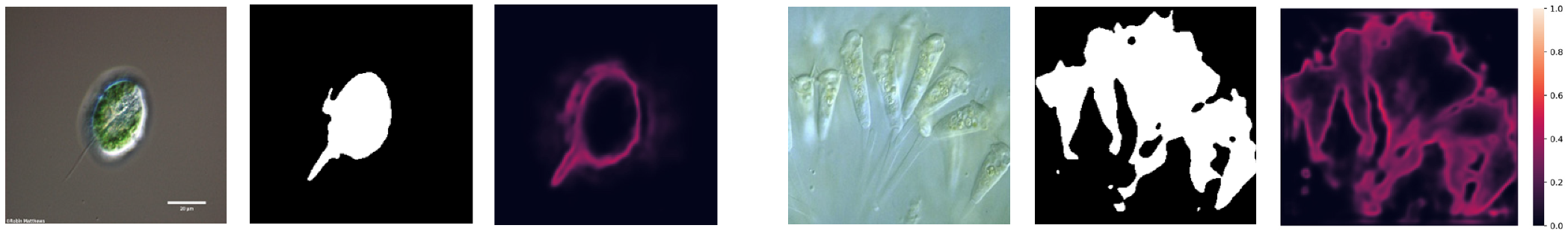
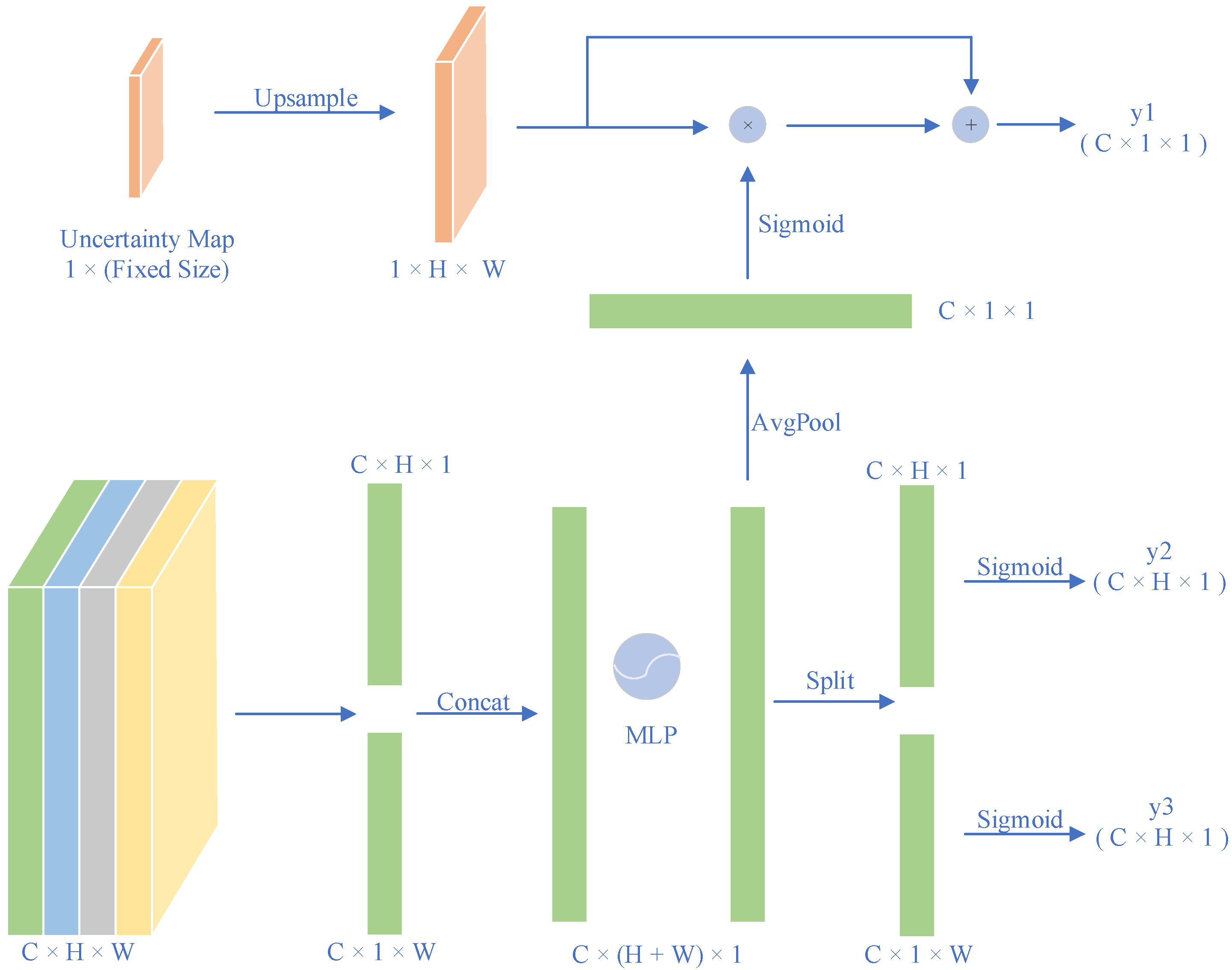
3.2. Uncertainty Revising Network

We improved the residual feedback network (RF-Net) proposed by Wang et al. [3], which is called the uncertainty revising network (UR-Net). The overall architecture of the network is shown in Figure 2, and the detailed parameters of each encoder, decoder, and other module within the network are presented in

Table 1. Detailed parameters of each module within the network. P: pooling; U: upsample; S: sigmoid.

Module	Architecture
		P	Convolutions	U	S	Notes
Initial encoder		√	(7 × 7, 64, stride = 2)			Similar to ResNet-50
Encoder	1	√	((1 × 1, 64) -> (3 × 3, 64) -> (1 × 1, 128)) × 3
	2	√	((1 × 1, 128) -> (3 × 3, 128) -> (1 × 1, 256)) × 4
	3	√	((1 × 1, 256) -> (3 × 3, 256) -> (1 × 1, 512)) × 6
	4	√	((1 × 1, 512) -> (3 × 3, 512) -> (1 × 1, 1024)) × 3
Decoder	4		(1 × 1, 128) -> (3 × 3, 128) -> (1 × 1, 512)	√		Pooling: (3 × 3), stride = 2 Upsample: scale factor = 2 ×n: repeat for n times
	3		(1 × 1, 64) -> (3 × 3, 64) -> (1 × 1, 256)	√
	2		(1 × 1, 32) -> (3 × 3, 32) -> (1 × 1, 128)	√
	1		(1 × 1, 16) -> (3 × 3, 16) -> (1 × 1, 64)	√
Final process			(3 × 3, 64) × 2 -> (3 × 3, 1)	√	√
Uncertainty feedback			(3 × 3, 64) -> (3 × 3, 1)		√
UpConv			(3 × 3, 64)	√		Resample to (128, 128)
Mid-pred	Mentioned below
Attention

. It is an encoder–decoder structure that has several differences from U-Net. First, for the encoders, a structure such as ResNet-50 is applied as the encoder rather than a double (3 × 3 Conv + Batchnorm + ReLU) to enhance the accuracy, together with fewer channels to ease the training and prediction process. Each encoder block contains x_i encoder units (where x_i ∈ {3, 4, 6, 3} and i ∈ {2, 3, 4, 5}), and each encoder unit is combined with two 3 × 3 convolutional layers. In encoder1, the encoder unit only contains a 7 × 7 convolutional layer. After each convolution, batch normalization and ReLU activation are performed. The other encoders (2, 3, 4, 5) had similar structures to the ResNet-50 but different channel numbers of outputs; more details can be found in Table 1. We also transformed the skip connection method from concatenation to element-wise addition. Each decoder block contains a 1 × 1 convolution to reduce the number of channels, an up-sampling layer to match the resolution, a 3 × 3 convolution to decode, and a 1 × 1 convolution to expand the channel size. The uncertainty feedback module primarily uses the information learned from the encoder to measure the probability of the prediction error or confusion rate of a particular area. It outputs uncertainty feedback that predicts the difference between the first inference result and the reality. As shown in Figure 3, the heatmap illustrates the possibility of a prediction failure for each pixel. It also shows the extent to which a position should be emphasized during the second stage of inference. This output participates in the next prediction step using the original image and this input data. Data from each decoder were applied with 3 × 3 convolution to be set to 64 channels and a bilinear up-sampling layer to ensure the cohesive scale and then concatenated together. Subsequently, two 3 × 3 convolutions reduce the concatenation result from 256 channels to 64 channels to one channel, and the result is activated with a sigmoid function. To illustrate the difference between the proposed UR-Net and RF-Net, two points were marked. First, the UR-Net integrated the attention module and mid-pred module within the network, and the proposed attention module was formed as an adapter to dynamic weighting rather than normal element-wise multiplication and addition.

3.3. Attention Module

Owing to the complicated structure and low contrast of the boundaries of environmental microorganisms, we designed an attention module at each scale of the encoder to enhance the segmentation results without too many parameters. The attention module is shown in Figure 4. First, we used global average pooling to encode the horizontal and vertical information from the entire picture. Hence, the output of the channel at height H and width W can be formulated as (C × H × 1) and (C × 1 × W), respectively.

The two channels of information are then concatenated as a (C × (H + W) × 1) vector. The feature map was then sent to a multilayer perception function to extract the importance of each row and column, which affected a single pixel when considered together. This function generates another vector, (C × (H + W) × 1). The vector is sent in two directions: it is applied with average pooling, forming a C × 1 × 1 vector y1 that indicates how the residual mask should be emphasized on the channel. It is also split into a C × H × 1 vector y2 and a C × 1 × 2 vector y3, which shows the positional interest of each pixel.

Processed by the attention module, the feature map x is rebalanced with weight $F\left(x\right)$, as follows:

$$F\left(x\right) = x\times \left(1+ y2\times y3 + y1\times residual\_mask\right)$$

(1)

Note that even if no residual mask is produced by the uncertainty feedback module in the first inference of the encoder–decoder, the proposed attention module can still be treated as a normal attention mechanism without failure. In the second inference stage of the encoder–decoder, the proposed attention mechanism can dynamically assign additional weights to each channel according to the data of the uncertainty feedback module, and then more accurate segmentation results can be obtained.

3.4. Mid-Pred Module

To train deeper networks more efficiently, we designed a mid-pred module in our networks after each decoder, inspired by previous studies. Wang et al. [38] adopted an additional supervision loss branch from the main network as an additional strategy. With this strategy, predictions are directly achieved from the middle layers of the networks and are optimized by loss functions [39]. They also utilized a similar strategy and achieved higher Dice scores in their networks for multiple segmentation datasets.

Therefore, according to the aforementioned compelling strategy, we developed a mid-pred module for our UR-Net. Each mid-pred module on a certain level uses the output of the decoder on the same level and generates a rough prediction with a lower resolution of the image (mid-prediction). The ground truth is resampled to the same resolution for calculating loss. While optimizing the model, the mid-pred module can shorten the path from the ground truth to each module. This can reduce the problem of gradient vanishing and improve the segmentation result.

More specifically, the architecture of the mid-pred module is as follows: the first two 3 × 3 convolution layers in each mid-pred module were reduced to half of the channels and then to only one channel because the channels of each decoded output were not the same. The results were then activated using a sigmoid function. Simultaneously, the mid-pred modules were also optimized using a loss function. In summary, the mid-pred module for the network is formed as follows:

$$F \left(x\right) = Sigmoid \left(f^3\left(x\right)\right)$$

(2)

where $f^3$ denotes convolutions that reduce the number of channels and extract features.

3.5. Loss Function

The proposed UR-Net has different auxiliary predictions from the decoder and the uncertainty adjustment module and more discriminating features can be obtained. To further capture this advantage and optimize the learning effect, we propose a multi-loss function that contains three sub-loss parts between the prediction and ground truth.

There are three types of sub-loss that correlate three parts of the prediction results from the two stages of the network. First, in each inference stage of the encoder–decoder, the segmentation result from the network is presented as $P^i$. We applied a weighted-balanced loss function, $L_{wbl}$ [40], which penalizes pixels in both the background and EM areas. Owing to the inconsistency in the size and shape of different images, the weight-balanced parameter can adjust the class imbalance. The loss function is expressed as follows:

$$L_{wbl}=1-w\frac{{{\displaystyle \sum }}_{n=1}^{N^1}{p}_n{y}_n}{{{\displaystyle \sum }}_{n=1}^{N_1}\left(p_n+y_n\right)}-\left(1-w\right)\frac{{{\displaystyle \sum }}_{n=1}^{N_0}\left(1-p_n\right)\left(1-y_n\right)}{{{\displaystyle \sum }}_{n=1}^{N_0}\left(2-p_n-y_n\right)}$$

(3)

where $N_0$, $N_1$ denotes the pixels where $y_n$ = 0,1, and $w$ = $N_0$/($N_0$+$N_1$) is the weight-balancing parameter calculated beyond. $p_n$ is the probability of pixels by prediction. Each prediction result is adjusted using a loss function.

Second, our uncertainty feedback module extracts the prediction failure rate from the decoder, which is denoted as $U$. To describe the actual failure rate, we used $U^{\prime }$ as the difference between the first stage of the prediction result P¹ and the ground truth. To sum up, the $U^{\prime }$ is formulated as follows:

$$U^{\prime }=\left|P^1-GT\right|$$

(4)

The uncertainty feedback was adjusted using a binary cross-entropy function, $L_{bce}$. The loss function can be calculated as shown below:

$$L_{bce}=-\left[y_n\cdot \log x_n+\left(1-y_n\right)\cdot \log \left(1-x_n\right)\right]$$

(5)

where $x_n$ denotes the prediction result and $y_n$ denotes the reality.

Finally, for the mid-pred part, we applied PolyLoss [41]. The PolyLoss provides a unified view of the multiple common loss functions. The loss is designed based on the Talor expansion of the CE and the focal losses. The poly-1 loss is a simplification of the loss function, which depends on only one hyperparameter to be fine-tuned on different datasets to achieve better performance. The equation is shown below:

$$L_{\mathrm{Poly}-\mathrm{l}}=L_{\mathrm{CE}}+{ϵ}_1\left(1-P_t\right), Pt=\left|yt-pt\right|$$

(6)

Generally, the final loss is combined with the aforementioned sub-losses, which are calculated as follows:

$$L=L_{bce}\left\{U,U^{\prime }\right\} + {\displaystyle \sum }_{i=1}^2(2\times L_{wbl}\left\{P^i,GT\right\}+ {\displaystyle \sum }_{j=1}^3{L}_{\mathrm{poly}}\left\{M_j^i, GT\right\})$$

(7)

where $L_x$ is the x-type loss function; $U$ is the uncertainty of prediction and $U^{\prime }$ is the actual possibility of prediction failure; $P^i$ and $M_j^i$ indicate each stage and level of prediction (prediction and mid-prediction), respectively; and $GT$ shows the ground truth.

4. Experiments and Analysis

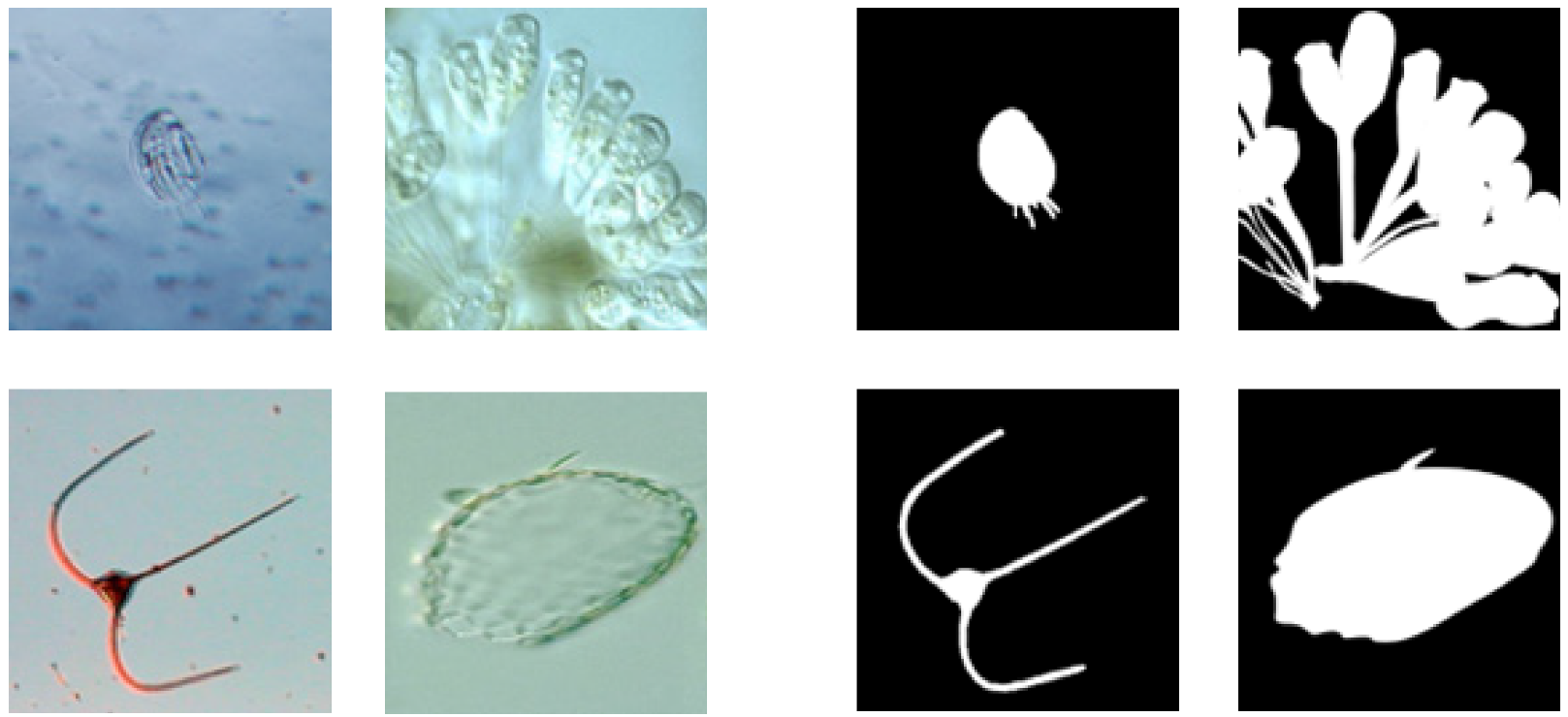
4.1. Experimental Datasets and Preprocessing

The EMDS-6 [37] dataset was used for the comparison. It consisted of EM images captured using a microscope. In the dataset, EMs were divided into 21 types, each of which included 40 pairs of original and ground truth images. Of the samples, 70% were randomly selected from each category for training, 10% for validation, and 20% for testing. For each sample, we resized it to a resolution of 256 × 256 and applied multiple augmentations of a random flip of 0.5 possibilities for each horizontal and vertical, rotation from −10 to 10, scale from 0.8 to 1.2, and translation of (0, 0.1) to improve the generalization of our model.

4.2. Experimental Setup and Evaluation

For the experimental environment, we used the open-source PyTorch toolkit and the MMSegmentation toolkit for comparison and ablation studies. We adopted the adaptive moment estimation of Kingma et al. [42] with beta1 = 0.9, beta2 = 0.999, and epsilon = ${10}^{-8}$ to optimize our networks. We trained the networks on NVIDIA TITAN Xp with a minibatch of 16. The initial learning rate was $5\times {10}^{-5}$, multiplied by 0.99 for each epoch, and the networks were trained for a total of 120 epochs. We initialized the parameters as the Kaiming normal [43] to avoid gradient vanishing or explosion. Finally, we used the open-source sklearn and medpy toolkits to evaluate the results using the metrics provided in the toolkits.

For a quantitative comparison, we selected seven types of widely used evaluation metrics, i.e., accuracy, Dice, Jaccard, recall, ASD, HD95, and precision. Specifically, the accuracy measures the total number of correctly predicted pixels. The Dice score, which is mathematically equal to the F1 score, indicates the similarity between the prediction and ground truth. It is equal to twice the area of overlap divided by the total number of positive pixels in both the images. Jaccard is another name for IoU (intersection over union), which counts the overlap area in the union area. Precision shows the ratio of a true positive result to the entire positive prediction result, whereas recall reveals the proportion of true positive results in the positive part of the ground truth. ASD (average surface distance) is the average of all distances from points on predicted edges to the ground truth. HD95 shows the Hausdorff distance between the boundaries of prediction and ground truth but is more robust because it excludes extreme circumstances.

Note that, for accuracy, Dice, Jaccard, recall, and precision, a higher value indicates better results, whereas for ASD and HD95, a lower value indicates better results. The equations for these metrics are presented in

Table 2. Formulas for each evaluation metric.

Evaluation Indicators	Formula	Note
Accuracy	$\mathrm{Accuracy}=\frac{TP+TN}{TP+FP+TN+FN} \left(8\right)$	$TP:True Positive$ $TN:True Negative$ $FP:False Positive$ $FN:False Negative$ $X:Prediction$ $Y:Ground Truth$
Dice	$DSC=\frac{2\times \mid X\cap Y\mid }{\mid X\mid +\mid Y\mid } \left(9\right)$
Jaccard	$\mathrm{Jaccard}=\frac{\mid X\cap Y\mid }{\mid X\mid +\mid Y\mid -\mid X\cap Y\mid } \left(10\right)$
Recall	$\mathrm{Recall}=TPR=\frac{TP}{TP+FN} \left(11\right)$
Precision	$\mathrm{Precision}=\frac{TP}{TP+FP} \left(12\right)$
ASD	$\mathrm{ASD}={{\displaystyle \sum }}_{x\in X}mi{n}_{y\in Y}d\left(x,y\right)/\mid X\mid \left(13\right)$
HD95	$\mathrm{HD}95=ma{x}_{k95\%}\left[d\left(X,Y\right),d\left(Y,X\right)\right] \left(14\right)$

.

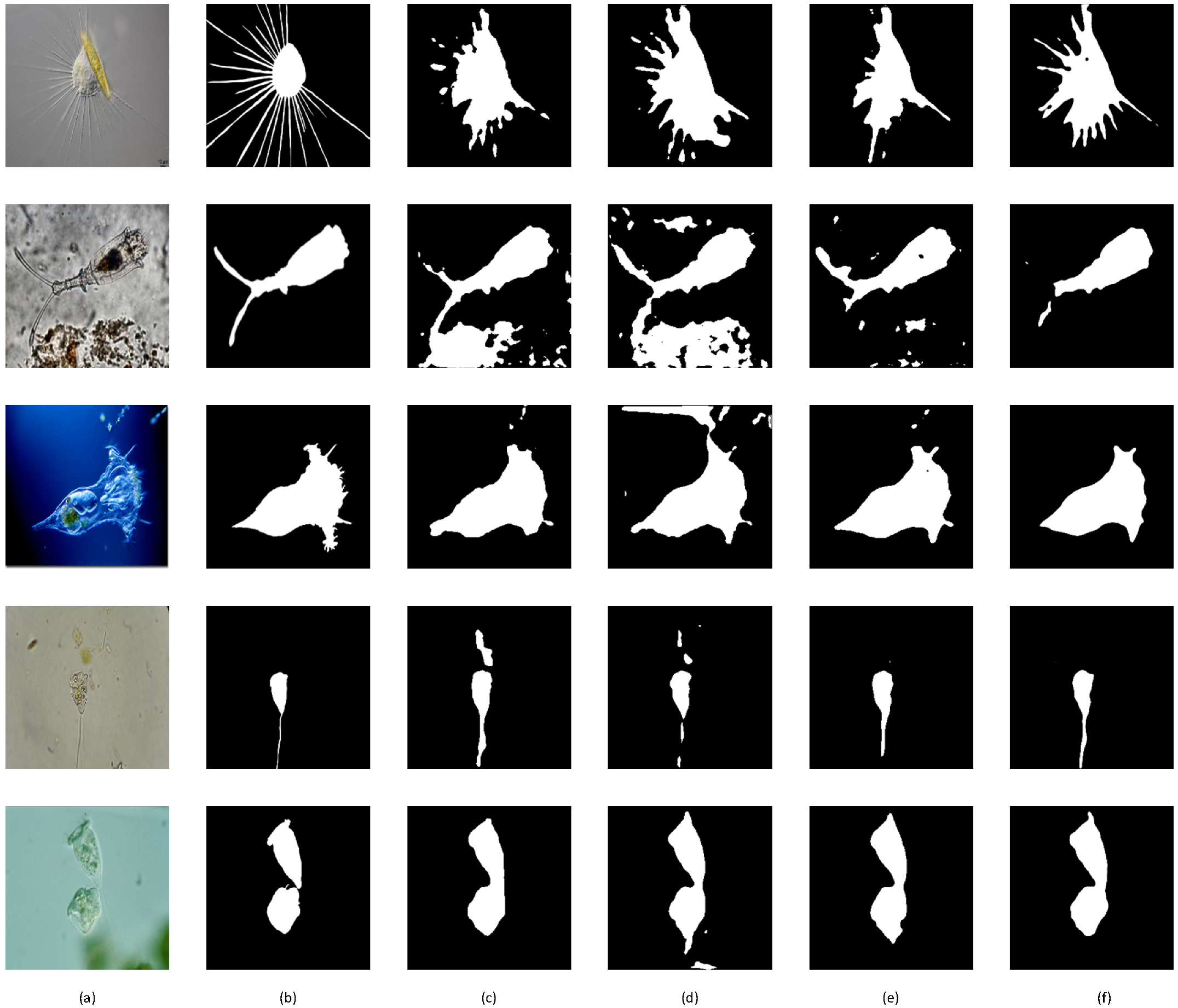
4.3. Ablation Experiment

To examine the effectiveness of each module, we conducted four ablation experiments to evaluate the contribution of each module. First, a residual feedback network was selected as the baseline. Subsequently, mid-pred and attention modules were successively added to the network. Finally, based on the same network, we added multiple losses to optimize the performance, that is, the proposed UR-Net. The experimental results are listed in

Table 3. Ablation experiment with the proposed method. MP: mid-pred module; A: attention module; ML: multi-loss.

Network	Accuracy	Dice	Jaccard	Recall	ASD	HD95	Precision
Baseline	94.48%	87.57%	77.89%	94.64%	0.88	4.55	81.48%
Baseline + MP	94.55%	87.81%	78.28%	95.53%	0.97	3.95	81.25%
Baseline + MP + A	95.40%	89.27%	80.61%	93.13%	0.62	3.04	85.71%
Baseline + MP + A + ML	95.63%	89.90%	81.65%	94.68%	0.59	2.24	85.58%

. To provide a more intuitive visual comparison, a schematic of the segmentation is presented in Figure 5.

Based on a comprehensive analysis of Figure 5 and Table 3, the following conclusions can be drawn.

First, Table 3 shows a steady increase in all metrics, indicating that our proposed modules have a positive effect on the segmentation results. Compared with the baseline, our mid-pred module shows improvements in accuracy (0.07%), Dice (0.24%), Jaccard (0.39%), and especially recall (0.89%); the attention module caused an obvious increment in accuracy (0.85%), Dice (1.46%), Jaccard (1.33%), and precision (4.46%) and a decline in ASD (0.35) and HD95 (0.89) and a small drop in recall (−1.23%); multi-loss further improved the accuracy (0.23%), Dice (0.63%), Jaccard (1.04%), ASD (0.03), and HD95 (0.80) and enhanced the recall from the previous part (1.55%) with a small cost to precision (0.13%).

Second, as shown in Figure 5, the prediction affected by the mid-pred module had the largest range of targets, and the recall value showed the same tendency. This is because the mid-pred module has a coarse-grained prediction with a low resolution, which tends to aggressively determine areas to be the foreground. This can better relate the transparent areas of microorganisms to the opaque ones. This is reasonable because the module can determine the rough area of the Ems. Although some Ems have transparent parts, the mid-pred module can locate them to achieve an accurate segmentation.

Third, the attention module extracted the target area more precisely, and from visual comparisons, we can see that the mispredicted areas were mostly removed. This is because the attention module can easily determine the location of the EM and discard the irrelevant parts. From the data, we can see a leap in most evaluation metrics, particularly in terms of the surface distance indicators. The only drop in recall is also acceptable because the positive area has been reduced significantly.

Finally, our multi-loss method fine-tuned the segmentation results and achieved the best performance for most metrics. The proposed loss function can effectively accelerate the training with higher accuracy. In the visual comparison, we can see that the segmentation results are not only more precise but also often have sharp and smooth edges.

To further perform a computational complexity analysis, we used the FLOPs (floating point operations per second) and parameter size as evaluation indicators for computational consumption, and the results are reported in

Table 4. Computational complexity analysis for ablation study. $1\mathrm{G}=2^{30};1\mathrm{M}=2^{20}$.

Network	FLOPs	Params
Baseline	16.38 G	22.01 M
Baseline + MP	16.96 G	22.50 M
Baseline + MP + A	16.98 G	22.77 M
Baseline + MP + A+ML	16.98 G	22.77 M

. The mid-pred module spent an additional 0.58 GFLOPs and 0.49 M param size; the attention module only costed approximately 0.02 GFLOPs and 0.27 M param size. Compared with significant improvements, these costs are affordable.

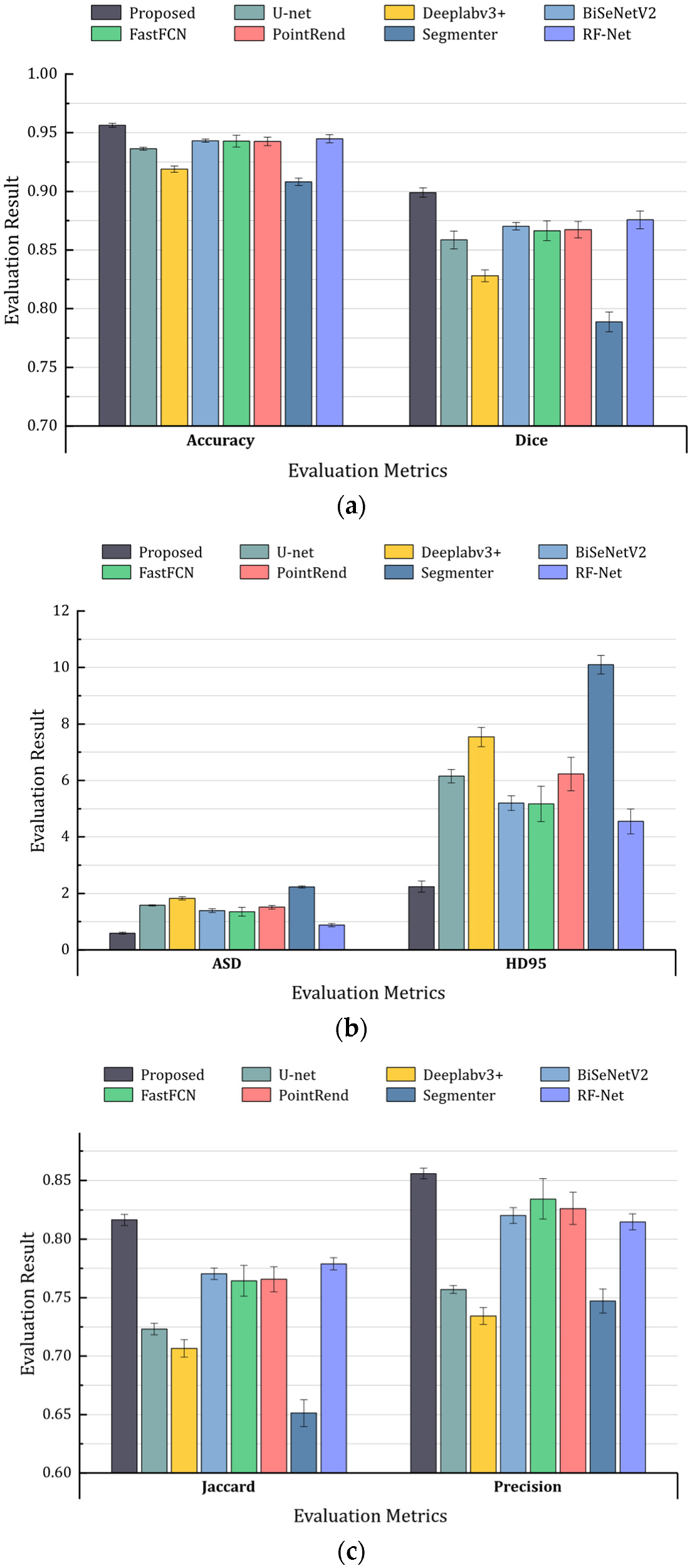
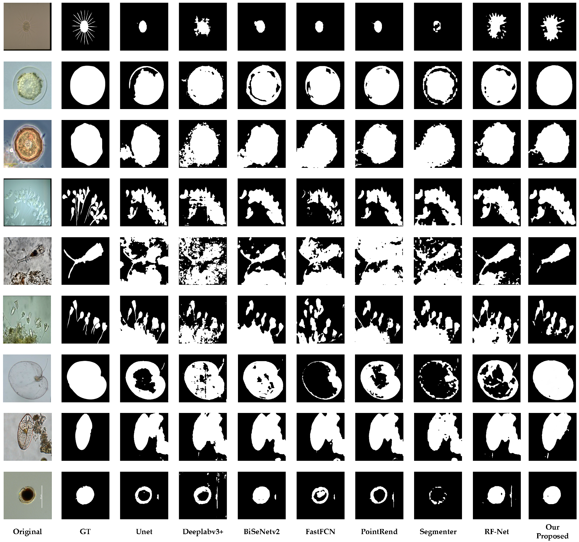
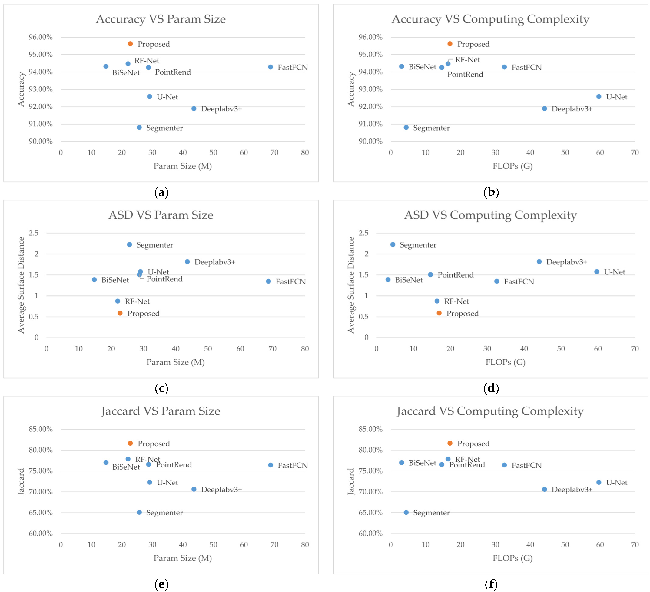
4.4. Comparison with the Latest Methods

For a complete comparison, we selected two commonly used networks (U-Net [14] and Deeplabv3+ [44]) and the four latest semantic segmentation networks (BiSeNetv2 [45], FastFCN [46], PointRend [47], and Segmenter [48]), all of which achieved the state of the art for semantic segmentation while publishing. For a fair comparison, we used the open-source MMSegmentation toolkit for all models.

The experimental results for the compared methods are listed In

Table 5. Evaluation results of the compared methods. Bold means the best value.

	Accuracy	Dice	Jaccard	Recall	ASD	HD95	Precision
Proposed	95.63%	89.90%	81.65%	94.68%	0.59	2.24	85.58%
U-Net	92.59%	83.93%	72.31%	94.16%	1.58	6.15	75.70%
Deeplabv3+	91.90%	82.80%	70.65%	94.92%	1.82	7.54	73.42%
BiSeNetv2	94.32%	87.03%	77.04%	92.68%	1.39	5.2	82.03%
FastFCN	94.29%	86.64%	76.44%	90.11%	1.35	5.17	83.44%
PointRend	94.26%	86.73%	76.58%	91.29%	1.51	6.23	82.62%
Segmenter	90.81%	78.87%	65.12%	83.54%	2.23	10.1	74.70%
RF-Net	94.48%	87.57%	77.89%	94.64%	0.88	4.55	81.48%

, where the values marked in bold indicate the best performance. For visual purposes, we provide a comparison diagram for the actual segmentation effect of the different methods, as shown in Figure 6 and Figure 7.

From the above results, the proposed network achieves the highest score in terms of accuracy, Dice, Jaccard, and precision compared with other networks, which shows its outstanding performance compared with other SOTAs (state-of-the-arts). For example, compared with the recent work PointRend, we obtained an accuracy improvement of 1.37%, Dice score of 3.17%, Jaccard score of 5.07%, recall rate of 3.39%, precision of 2.96%, ASD of 0.92%, and HD95 of 3.74%. We also surpassed the classic model (such as U-Net and Deeplabv3+) and recent popular methods (BiSeNet, PointRend, and Segmenter) for almost all metrics. In particular, our results are significantly better for the ASD metric, which indicates competitive performance in terms of robustness and higher boundary localizing ability.

Visual comparisons also proved that the proposed model generally achieves a sharp and smooth segmentation result and that the segmented foreground and background are closer to human vision than other models. It is worth mentioning that for EMs with transparency, our proposed network is more capable of filling the entire part, whereas the other networks commonly show hollows. Furthermore, when encountering a complex background, other networks falsely emphasize useless regions. However, the proposed network efficiently filters them out.

Another interesting phenomenon is that the newly proposed transformer-based model Segmenter did not perform well on this dataset. In our opinion, although transformers have a strong potential for semantic segmentation, in specific cases with less data, such as microorganisms, a specially designed model is required.

To further compare the time complexity, we report the FLOPs and parameter memory as the evaluation indicators for the comparison method in

Table 6. Computational complexities of different methods for comparative study.

Network	FLOPs	Params
Proposed	16.98 G	22.77 M
U-Net	59.64 G	29.06 M
Deeplabv3+	44.05 G	43.58 M
BiSeNetv2	3.09 G	14.78 M
FastFCN	32.56 G	68.70 M
PointRend	14.61 G	28.73 M
Segmenter	4.40 G	25.68 M
RF-Net	16.38 G	22.01 M

. To provide a more intuitive and comprehensive comparison, we also draw a diagram of the performance requirements versus segmentation capabilities in Figure 8.

It is worth mentioning that the proposed method has moderate param size and operation count. From Table 6, we can see that our proposed network has significantly lower FLOPs and param sizes than classical networks, such as U-Net and Deeplabv3+. Figure 8 shows a balanced tradeoff between the computing requirements and segmentation performance. It is worth mentioning that the BiSeNetv2 has a decent segmentation result with small sizes. From our analysis, it has a detail branch and a semantic branch to individually handle fine-grained and coarse-grained features, which correlates our mid-pred module. From the visual comparison, we can also see the fewer holes inside the EMs predicted. However, compared with the newly proposed networks, our proposed method has a moderate performance requirement in terms of hardware but better segmentation results, in terms of both evaluation metrics and human observation.

5. Conclusions

In this study, we proposed a U-Net-like network for environmental microorganism image segmentation. First, we proposed an uncertainty revising network that adds a mid-pred module to locate foreground areas. Subsequently, an attention module that can extract precise localization information for positioning and range control was proposed. Finally, multi-loss was used for optimization to enhance the robustness of the network. The experimental results demonstrate that the proposed method compares favorably with SOTAs and is outstanding in terms of segmentation quality and speed. Therefore, it satisfies the requirements of stability and real-time automatic detection.

References

1. Pepper, I.L.; Gentry, T.J. Microorganisms Found in the Environment. In Environmental Microbiology; Elsevier: Amsterdam, The Netherlands, 2015; pp. 9–36. [Google Scholar]
2. Buszewski, B.; Rogowska, A.; Pomastowski, P.; Z\loch, M.; Railean-Plugaru, V. Identification of Microorganisms by Modern Analytical Techniques. J. AOAC Int. 2017, 100, 1607–1623. [Google Scholar]
3. Luo, Z.; Yang, W.; Gou, R.; Yuan, Y. TransAttention U-Net for Semantic Segmentation of Poppy. Electronics 2023, 12, 487. [Google Scholar] [CrossRef]
4. Wang, K.; Liang, S.; Zhang, Y. Residual Feedback Network for Breast Lesion Segmentation in Ultrasound Image. In Proceedings of the International Conference on Medical Image Computing and Computer-Assisted Intervention, Strasbourg, France, 27 September–1 October 2021; Springer: Berlin/Heidelberg, Germany, 2021; pp. 471–481. [Google Scholar]
5. Otsu, N. A Threshold Selection Method from Gray-Level Histograms. IEEE Trans. Syst. Man Cybern. 1979, 9, 62–66. [Google Scholar]
6. Nock, R.; Nielsen, F. Statistical Region Merging. IEEE Trans. Pattern Anal. Mach. Intell. 2004, 26, 1452–1458. [Google Scholar]
7. Kanungo, T.; Mount, D.M.; Netanyahu, N.S.; Piatko, C.D.; Silverman, R.; Wu, A.Y. An Efficient K-Means Clustering Algorithm: Analysis and Implementation. IEEE Trans. Pattern Anal. Mach. Intell. 2002, 24, 881–892. [Google Scholar]
8. Najman, L.; Schmitt, M. Watershed of a Continuous Function. Signal Process. 1994, 38, 99–112. [Google Scholar]
9. Boykov, Y.; Veksler, O.; Zabih, R. Fast Approximate Energy Minimization via Graph Cuts. IEEE Trans. Pattern Anal. Mach. Intell. 2001, 23, 1222–1239. [Google Scholar]
10. Plath, N.; Toussaint, M.; Nakajima, S. Multi-Class Image Segmentation Using Conditional Random Fields and Global Classification. In Proceedings of the 26th Annual International Conference on Machine learning, Montreal, QC, Canada, 14–18 June 2009; pp. 817–824. [Google Scholar]
11. Li, S.Z. Ch. 13. Modeling Image Analysis Problems Using Markov Random Fields. Handb. Stat. 2003, 21, 473–513. [Google Scholar]
12. Gabaix, X. A Sparsity-Based Model of Bounded Rationality. Q. J. Econ. 2014, 129, 1661–1710. [Google Scholar]
13. Long, J.; Shelhamer, E.; Darrell, T. Fully Convolutional Networks for Semantic Segmentation. In Proceedings of the IEEE Conference on Computer Vision and Pattern Recognition, Boston, MA, USA, 7–12 June 2015; pp. 3431–3440. [Google Scholar]
14. Ronneberger, O.; Fischer, P.; Brox, T. U-Net: Convolutional Networks for Biomedical Image Segmentation. In Proceedings of the International Conference on Medical Image Computing and Computer-Assisted Intervention, Munich, Germany, 5–9 October 2015; Springer: Berlin/Heidelberg, Germany, 2015; pp. 234–241. [Google Scholar]
15. Zhou, Z.; Siddiquee, M.M.R.; Tajbakhsh, N.; Liang, J. Unet++: Redesigning Skip Connections to Exploit Multiscale Features in Image Segmentation. IEEE Trans. Med. Imaging 2019, 39, 1856–1867. [Google Scholar]
16. Badrinarayanan, V.; Kendall, A.; Cipolla, R. Segnet: A Deep Convolutional Encoder-Decoder Architecture for Image Segmentation. IEEE Trans. Pattern Anal. Mach. Intell. 2017, 39, 2481–2495. [Google Scholar]
17. Chen, D.; Hu, F.; Mathiopoulos, P.T.; Zhang, Z.; Peethambaran, J. MC-UNet: Martian Crater Segmentation at Semantic and Instance Levels Using U-Net-Based Convolutional Neural Network. Remote Sens. 2023, 15, 266. [Google Scholar] [CrossRef]
18. Lin, G.; Milan, A.; Shen, C.; Reid, I. Refinenet: Multi-Path Refinement Networks for High-Resolution Semantic Segmentation. In Proceedings of the IEEE Conference on Computer Vision and Pattern Recognition, Honolulu, HI, USA, 21–26 July 2017; pp. 1925–1934. [Google Scholar]
19. Visin, F.; Kastner, K.; Cho, K.; Matteucci, M.; Courville, A.; Bengio, Y. ReNet: A Recurrent Neural Network Based Alternative to Convolutional Networks. arXiv 2015, arXiv:1505.00393. [Google Scholar]
20. Byeon, W.; Breuel, T.M.; Raue, F.; Liwicki, M. Scene Labeling with Lstm Recurrent Neural Networks. In Proceedings of the IEEE Conference on Computer Vision and Pattern Recognition, Boston, MA, USA, 7–12 June 2015; pp. 3547–3555. [Google Scholar]
21. Dosovitskiy, A.; Beyer, L.; Kolesnikov, A.; Weissenborn, D.; Zhai, X.; Unterthiner, T.; Dehghani, M.; Minderer, M.; Heigold, G.; Gelly, S.; et al. An Image Is Worth 16x16 Words: Transformers for Image Recognition at Scale. arXiv 2010, arXiv:11929 2020. [Google Scholar]
22. Vaswani, A.; Shazeer, N.; Parmar, N.; Uszkoreit, J.; Jones, L.; Gomez, A.N.; Kaiser, L.; Polosukhin, I. Attention Is All You Need. Adv. Neural Inf. Process. Syst. 2017, 30, 5998–6008. [Google Scholar]
23. Ranftl, R.; Bochkovskiy, A.; Koltun, V. Vision Transformers for Dense Prediction. In Proceedings of the IEEE/CVF International Conference on Computer Vision, Montreal, BC, Canada, 11–17 October 2021; pp. 12179–12188. [Google Scholar]
24. Hu, J.; Shen, L.; Sun, G. Squeeze-and-Excitation Networks. In Proceedings of the IEEE Conference on Computer Vision and Pattern Recognition, Salt Lake City, UT, USA, 18–23 June 2018; pp. 7132–7141. [Google Scholar]
25. Yang, C.; Wu, W.; Wang, Y.; Zhou, H. Multi-Modality Global Fusion Attention Network for Visual Question Answering. Electronics 2020, 9, 1882. [Google Scholar] [CrossRef]
26. Woo, S.; Park, J.; Lee, J.-Y.; Kweon, I.S. Cbam: Convolutional Block Attention Module. In Proceedings of the European conference on computer vision (ECCV), Munich, Germany, 8–14 September 2018; pp. 3–19. [Google Scholar]
27. Hou, Q.; Zhou, D.; Feng, J. Coordinate Attention for Efficient Mobile Network Design. In Proceedings of the IEEE/CVF Conference on Computer Vision and Pattern Recognition, Nashville, TN, USA, 19–25 June 2021; pp. 13713–13722. [Google Scholar]
28. Wu, J.; Liu, W.; Li, C.; Jiang, T.; Shariful, I.M.; Sun, H.; Li, X.; Li, X.; Huang, X.; Grzegorzek, M. A State-of-the-Art Survey of U-Net in Microscopic Image Analysis: From Simple Usage to Structure Mortification. arXiv 2022, arXiv:06465 2022. [Google Scholar]
29. Dubuisson, M.-P.; Jain, A.K.; Jain, M.K. Segmentation and Classification of Bacterial Culture Images. J. Microbiol. Methods 1994, 19, 279–295. [Google Scholar]
30. Kyan, M.; Guan, L.; Liss, S. Refining Competition in the Self-Organising Tree Map for Unsupervised Biofilm Image Segmentation. Neural Netw. 2005, 18, 850–860. [Google Scholar]
31. Kosov, S.; Shirahama, K.; Li, C.; Grzegorzek, M. Environmental Microorganism Classification Using Conditional Random Fields and Deep Convolutional Neural Networks. Pattern Recognit. 2018, 77, 248–261. [Google Scholar]
32. Hung, J.; Carpenter, A. Applying Faster R-CNN for Object Detection on Malaria Images. In Proceedings of the IEEE conference on computer vision and pattern recognition workshops, Honolulu, HI, USA, 21–26 July 2017; pp. 56–61. [Google Scholar]
33. Zhang, J.; Li, C.; Kosov, S.; Grzegorzek, M.; Shirahama, K.; Jiang, T.; Sun, C.; Li, Z.; Li, H. LCU-Net: A Novel Low-Cost U-Net for Environmental Microorganism Image Segmentation. Pattern Recognit. 2021, 115, 107885. [Google Scholar]
34. Aydin, A.S.; Dubey, A.; Dovrat, D.; Aharoni, A.; Shilkrot, R. CNN Based Yeast Cell Segmentation in Multi-Modal Fluorescent Microscopy Data. In Proceedings of the 2017 IEEE Conference on Computer Vision and Pattern Recognition Workshops (CVPRW), Honolulu, Hawaii, USA, 21–26 July 2017; pp. 753–759. [Google Scholar]
35. Ang, R.B.Q.; Nisar, H.; Khan, M.B.; Tsai, C.-Y. Image Segmentation of Activated Sludge Phase Contrast Images Using Phase Stretch Transform. Microscopy 2019, 68, 144–158. [Google Scholar]
36. Zhou, B.; Zhao, H.; Puig, X.; Xiao, T.; Fidler, S.; Barriuso, A.; Torralba, A. Semantic Understanding of Scenes through the ADE20K Dataset. Int. J. Comput. Vis. 2018, 127, 302–321. [Google Scholar]
37. Zhao, P.; Li, C.; Rahaman, M.M.; Xu, H.; Ma, P.; Yang, H.; Sun, H.; Jiang, T.; Xu, N.; Grzegorzek, M. EMDS-6: Environmental Microorganism Image Dataset Sixth Version for Image Denoising, Segmentation, Feature Extraction, Classification, and Detection Method Evaluation. Front. Microbiol. 2022, 13, 1334. [Google Scholar]
38. Wang, L.; Lee, C.-Y.; Tu, Z.; Lazebnik, S. Training Deeper Convolutional Networks with Deep Supervision. arXiv 2015, arXiv:1505.02496. [Google Scholar]
39. Zhao, X.; Zhang, P.; Song, F.; Ma, C.; Fan, G.; Sun, Y.; Feng, Y.; Zhang, G. Prior Attention Network for Multi-Lesion Segmentation in Medical Images. IEEE Trans. Med. Imaging 2022, 41, 3812–3823. [Google Scholar]
40. Wang, K.; Liang, S.; Zhong, S.; Feng, Q.; Ning, Z.; Zhang, Y. Breast Ultrasound Image Segmentation: A Coarse-to-Fine Fusion Convolutional Neural Network. Med. Phys. 2021, 48, 4262–4278. [Google Scholar]
41. Leng, Z.; Tan, M.; Liu, C.; Cubuk, E.D.; Shi, X.; Cheng, S.; Anguelov, D. PolyLoss: A Polynomial Expansion Perspective of Classification Loss Functions. arXiv 2022, arXiv:2204.12511. [Google Scholar]
42. Kingma, D.P.; Ba, J. Adam: A Method for Stochastic Optimization. arXiv 2014, arXiv:1412.6980. [Google Scholar]
43. He, K.; Zhang, X.; Ren, S.; Sun, J. Delving Deep into Rectifiers: Surpassing Human-Level Performance on Imagenet Classification. In Proceedings of the Proceedings of the IEEE International Conference on Computer Vision, Santiago, Chile, 7–13 December 2015; pp. 1026–1034. [Google Scholar]
44. Chen, L.-C.; Zhu, Y.; Papandreou, G.; Schroff, F.; Adam, H. Encoder-Decoder with Atrous Separable Convolution for Semantic Image Segmentation. In Proceedings of the European Conference on Computer Vision (ECCV), Munich, Germany, 17–24 May 2018; pp. 801–818. [Google Scholar]
45. Yu, C.; Gao, C.; Wang, J.; Yu, G.; Shen, C.; Sang, N. Bisenet v2: Bilateral Network with Guided Aggregation for Real-Time Semantic Segmentation. Int. J. Comput. Vis. 2021, 129, 3051–3068. [Google Scholar]
46. Wu, H.; Zhang, J.; Huang, K.; Liang, K.; Yu, Y. Fastfcn: Rethinking Dilated Convolution in the Backbone for Semantic Segmentation. arXiv 2019, arXiv:1903.11816. [Google Scholar]
47. Kirillov, A.; Wu, Y.; He, K.; Girshick, R. PointRend: Image Segmentation as Rendering. In Proceedings of the IEEE/CVF Conference on Computer Vision and Pattern Recognition, Seattle, WA, USA, 13–19 June 2020; pp. 9799–9808. [Google Scholar]
48. Strudel, R.; Garcia, R.; Laptev, I.; Schmid, C. Segmenter: Transformer for Semantic Segmentation. In Proceedings of the Proceedings of the IEEE/CVF International Conference on Computer Vision, Montreal, BC, Canada, 11–17 October 2021; pp. 7262–7272. [Google Scholar]
Figure 1. Different types of EMs. They have various shapes and sizes and often have vague edges because of their transparency and the lens being out of focus.
Electronics 12 00763 g001
Figure 2. Overall architecture of the network.
Electronics 12 00763 g002
Figure 3. Possibility of prediction failure calculated using the uncertainty feedback module.
Electronics 12 00763 g003
Figure 4. Architecture of the attention module.
Electronics 12 00763 g004
Figure 5. Visual comparison between baseline and improvement. (a) Original picture, (b) ground truth, (c) baseline, (d) baseline + MP, (e) baseline + MP + A, (f) baseline + MP + A + ML (our proposed model).
Electronics 12 00763 g005
Figure 6. Column chart for comparison results. (a): Accuracy and dice score; (b): ASD and HD95; (c): Jaccard score and Precision.
Electronics 12 00763 g006
Figure 7. Visual comparison of different networks.
Electronics 12 00763 g007
Figure 8. Performance requirements versus segmentation capabilities. (a) accuracy versus param size; (b) accuracy versus computing complexity; (c) ASD versus param size; (d) ASD versus computing complexity; (e) Jaccard score versus param size; (f) Jaccard score computing complexity.
Electronics 12 00763 g008