Methodological Research on Image Registration Based on Human Brain Tissue In Vivo

Abstract

As one of the critical steps in brain imaging analysis and processing, brain image registration plays a significant role. In this paper, we proposed a technique of human brain image registration based on tissue morphology in vivo to address the problems of previous image registration. First, different feature points were extracted and combined, including those at the boundary of different brain tissues and those of the maximum or minimum from the original image. Second, feature points were screened through eliminating their wrong matching pairs between moving image and reference image. Finally, the remaining matching pairs of feature points were used to generate the model parameters of spatial transformation, with which the brain image registration can be finished by combining interpolation techniques. Results showed that compared with the Surf, Demons, and Sift algorithms, the proposed method can perform better not only for four quantitative indicators (mean square differences, normalized cross correlation, normalized mutual information and mutual information) but also in spatial location, size, appearance contour, and registration details. The findings may suggest that the proposed method will be of great value for brain image reconstruction, fusion, and statistical comparison analysis.

1. Introduction

The brain, as the main part of the human nervous system, is the primary regulator for the life and working of the body [1]. Any lesion from the brain may cause a deficit or loss of a person’s part physiological functions and even threaten life. Therefore, brain research is of great value to clinical medicine. With the development of the society, a variety of imaging technologies have been greatly developed, such as computed tomography (CT), magnetic resonance image (MRI), positron emission tomography (PET), electroencephalogram (EEG), and others [2,3]. These techniques can reflect the functional metabolism or structural organization in living body through various perspectives, which makes it possible to study the brain in vivo.

Currently, there are many steps in brain imaging analysis and processing, mainly including skull stripping, segmentation, smoothing, registration, reconstruction, fusion, and statistical contrast analysis [4]. Brain image registration plays a significant role as an essential preprocessing step [5]. It can correct the variations in the body position from one patient’s multiple imaging sessions and the distortions caused by the imaging modality itself. It is a prerequisite for brain image reconstruction, fusion, and statistical contrast analysis [6,7]. Currently, brain image registration can be divided into two categories according to the target of registration: registration for different individuals and registration for multiple brain images of the same person. The former is to explore a series of transformation parameters for the spatial consistence of the brain shape, size, tissue location and anatomical structure from different individuals. The latter is to find a series of transformation parameters for spatial consistence of multiple kinds of images from the same person. Therefore, the former is much more complicated than the latter, and can have a significant effect on the results of studies about neurodegenerative brain diseases, tumor radiotherapy localization, preoperative planning, and image-guided surgical navigation [8,9]. Therefore, the current study aims to explore an efficient registration technique about brain imaging based on different individuals.

Brain image registration methods can be divided into rigid and non-rigid registration according to the type of the parameters about spatial transformation [8]. Rigid registration involves only translation and rotation, and is usually used in rigid structures such as skeletons. However, the brain structure is complex, and simple translation and rotation cannot show the nonlinear deformation in brain tissues and organs. Therefore, rigid registration is not suitable for the brain images. Non-rigid registration is divided into two main categories according to the feature extraction methods: voxel-based registration and feature-based registration. Voxel-based registration obtains the parameters of spatial transformation by the similarity of gray level between images, such as the Demons algorithm [10] and B-spline algorithm [11]. This kind of algorithm does not need to detect feature point, thus avoiding the registration error caused by the mismatch of feature points. However, it depends on all gray values within the images. This can not only limit the computing speed, but also have a huge difference from the target of brain image registration between different individuals. Feature-based methods perform image registration by a series of feature points, such as Sift algorithm [12], Surf algorithm [13], and Harris corner detection [14]. The quality of feature point extraction determines the effect of registration. It can effectively discard the redundant information within brain images and do not consider the gray value, which fit in with the brain image registration between different individuals. However, the low quality of key feature points or the mismatched pairs of feature points will lead to unsatisfactory or even totally wrong registration. By the emerging of deep learning-based approaches, they have changed the landscape of medical image processing research and achieved the state-of-art performances in many applications [15,16] including brain image registration. Recently, Fan, J. et al. [17] proposed a deep learning approach for image registration by predicting deformation from image appearance on brain image. Experiments on a variety of datasets showed promising registration accuracy and efficiency. Ma, Y. et al. [18] proposed an unsupervised deformable image registration network (UDIR-Net) for 3D medical images. Their experiments on brain MR images showed that UDIR-Net exhibited competitive performance against several methods (such as DIRNet, FlowNet, JRS-Net, Elastix, and VoxelMorph). Chen, J. et al. [19] presented ViT-V-Net, which bridges ViT and ConvNet to provide volumetric medical image registration. In brain MRI images, their proposed architecture achieved superior performance to several top-performing registration methods. Song, L. et al. [20] proposed a hybrid network which combines Transformer and CNN, and applied it to brain MRI images. They found that the method improved the accuracy by 1% compared with the VoxelMorph, ViT-V-Net, and SYMNet. The above studies have provided excellent effect on brain registration. However, deep leaning-based registration generally has relatively higher requirements for equipment, environment and data, and its results may vary with one-training iteration. Therefore, given the above, we improved the brain registration based on the traditional method rather than the deep learning method.

To improve the brain image registration, the study proposed a new method based on different brain tissues in vivo. First, the brain tissue segmentation was carried out to obtain different tissues including the white matter, gray matter, and cerebrospinal fluid, followed by performing the morphological edge detection of different brain tissues. The key feature points were then extracted from each brain tissue and the original brain image and consisted of a set of feature points, followed by removing mismatched pairs of feature points by a random sample consensus (RANSAC) algorithm [21,22]. Finally, the registration parameters can be obtained depending on the remaining matched pairs of feature points, and be used for the final brain image registration. The registration method fully considers the morphological and spatial variability of individual brain tissues, dramatically improving the registration accuracy of brain images.

2. Materials and Methods

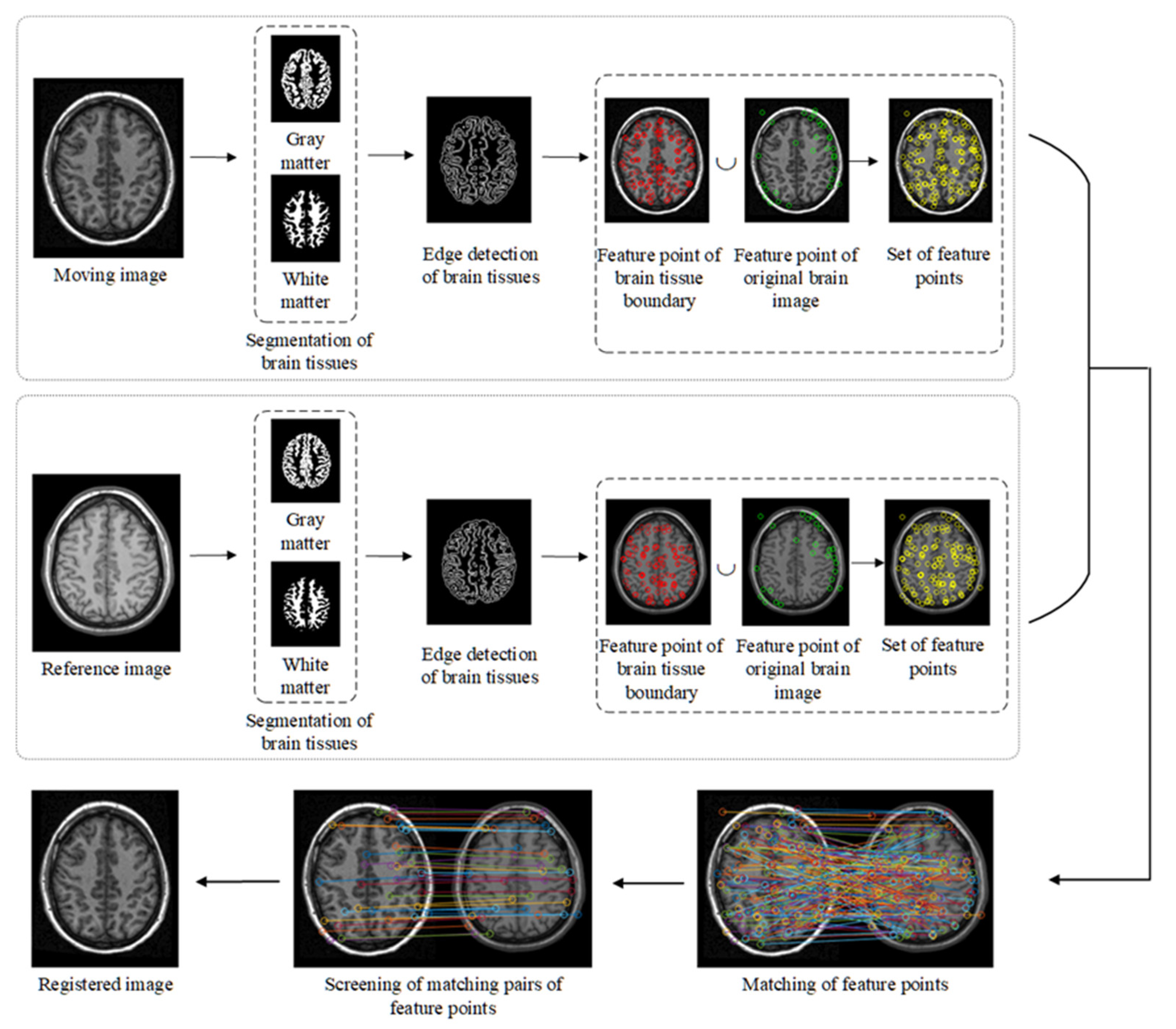
2.1. Algorithm Description

The brain image registration technique proposed in this study mainly includes brain tissue segmentation, morphological edge detection of different brain tissues, corner detection, detection of feature points, screening of feature points, and spatial transformation. The flow chart of the implementation is shown in Figure 1.

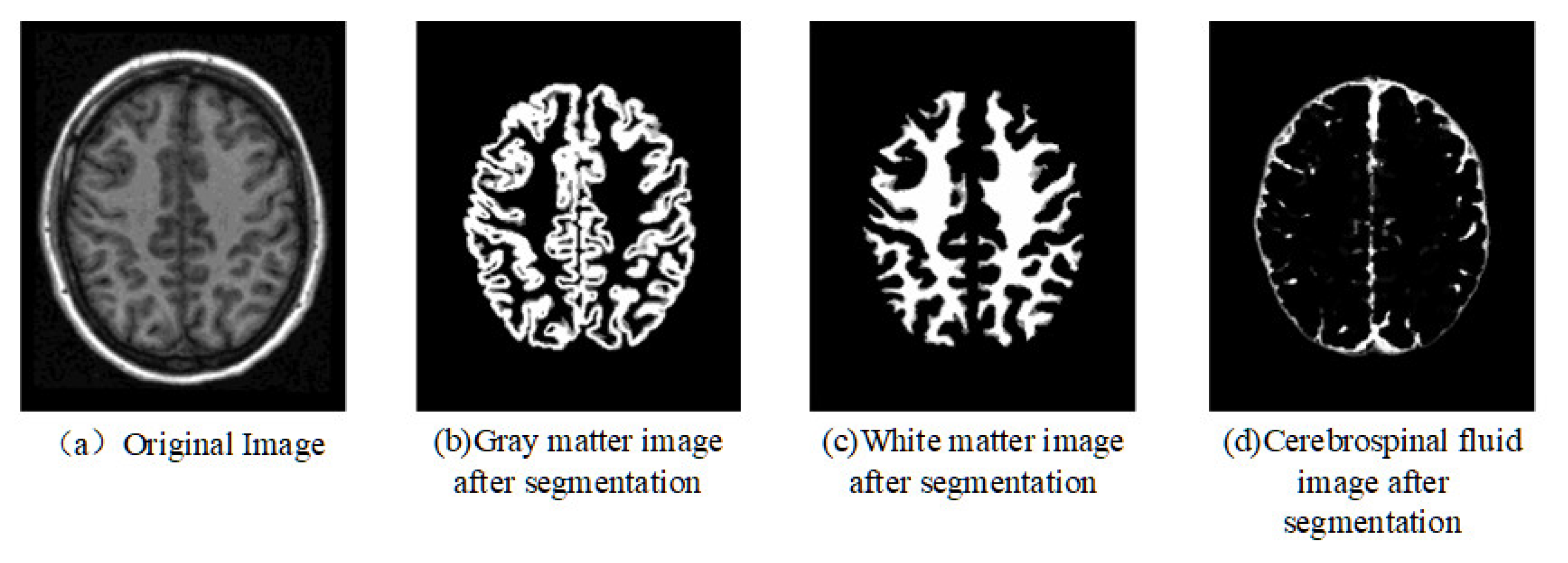
2.1.1. Segmentation of Brain Tissues

The current study is carried out based on brain T1 image. First, the T1 image was skull stripped, which is based on the FSL (https://fsl.fmrib.ox.ac.uk/fsl/fslwiki/ (accessed on 1 July 2022)) software. The skull-stripped T1 image was segmented into gray matter and white matter maps based on the Gaussian mixture model and Naive Bayes. The Gaussian mixture model determines the tissue class of each voxel within the brain based on maximum a posterior probability(MAP) [23]. If a given voxel has the highest posterior probability for a tissue category, the voxel is assigned to the tissue category [24,25]. Each brain image includes large number of voxels, and how to determine the category of each voxel is described in detail below. When all voxels are mixed, each voxel follows a total distribution. This distribution is not a Gaussian distribution but a Gaussian mixture model (a superposition of multiple Gaussian distributions). The Expectation Maximization (EM) algorithm [25] was used to estimate the parameters of each distribution in the mixed Gaussian model, which corresponds to the parameters of the probability distribution of voxel values within each tissue in this study. Suppose that each tissue’s distribution parameters have been estimated (that is to say, the probability of each voxel within each tissue is known), every voxel can be marked through Native Bayes model, which describes which brain tissue the voxel belongs to. The Bayesian formula is shown in Equation (1).

$$\mathrm{P}\left(\mathrm{A}\right|\mathrm{B})=\frac{\mathrm{P}\left(\mathrm{B}\right|\mathrm{A})\times \mathrm{P}\left(\mathrm{A}\right)}{\mathrm{P}(\mathrm{B})}$$

(1)

where A is one of the gray matter, white matter, or cerebrospinal fluid. B represents one voxel. P(A|B) and P(B|A) are the conditional probability. P(A) is the prior probability of tissue A, obtained from the tissue probability map (TPM) [26]. P(B) is the total probability.

Figure 2 shows an example of brain tissue segmentation for any one brain T1 image, which can demonstrate the effectiveness of the segmentation of the brain tissues.

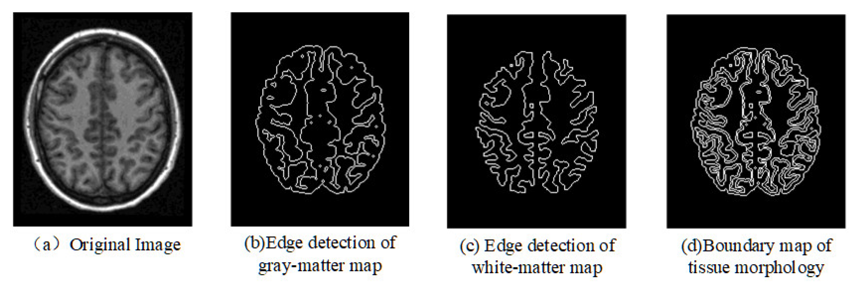
2.1.2. Edge Detection of Brain Tissues

After tissue segmentation, morphological filtering, threshold segmentation, and edge detection are used to obtain the morphological edge of individual brain tissues. First, the maps of individual brain’s white matter tissue and gray matter tissue are converted into binary maps. Next, filling, expanding, and edge detection for the binary maps are performed to obtain the edge images of different brain tissues. Finally, the merging of edge images from white matter and gray matter generates individual boundary image of tissue morphology, as shown in Figure 3.

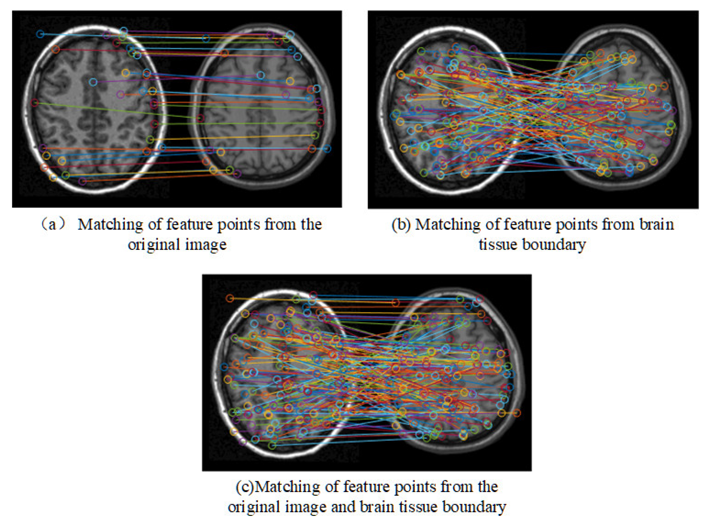
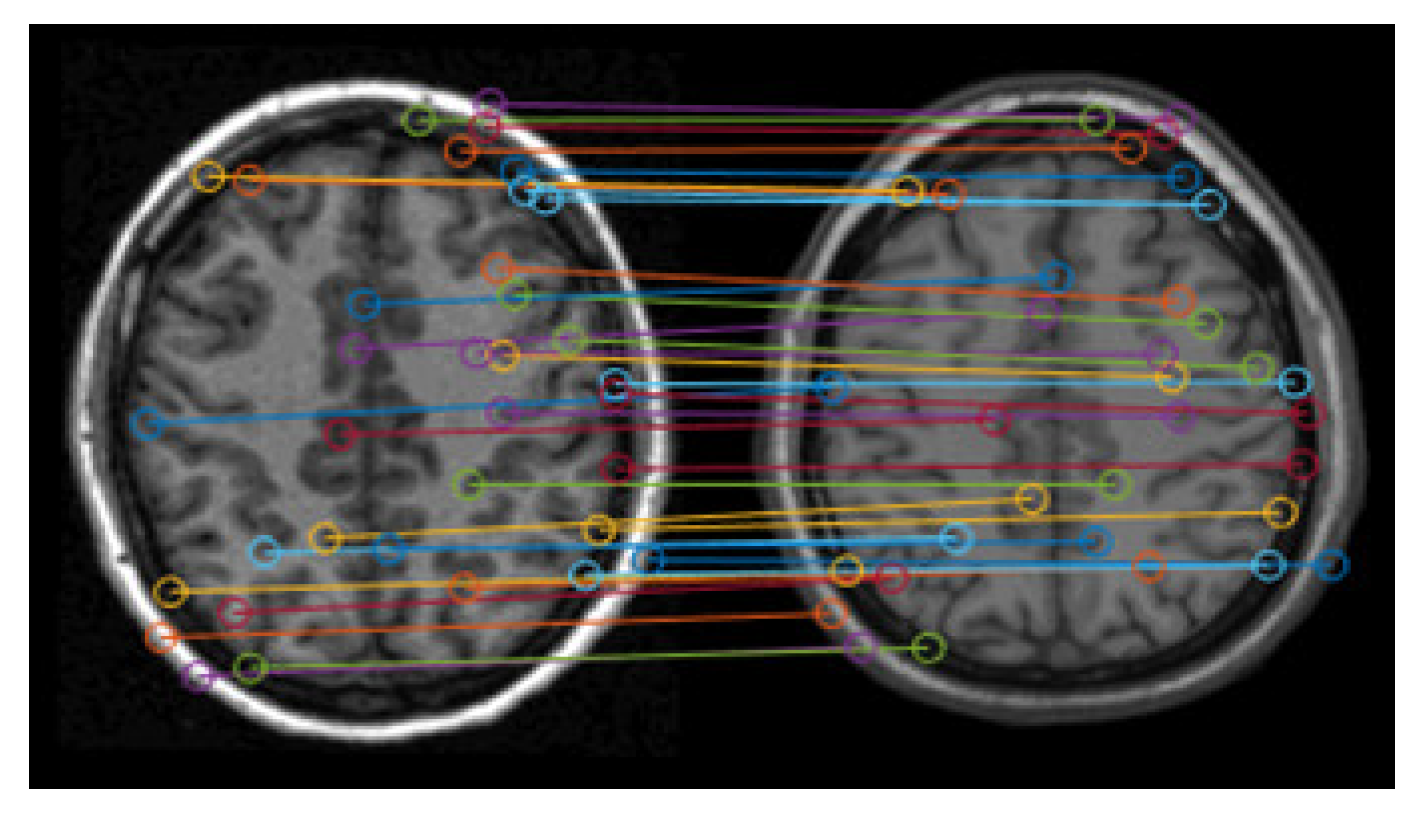
2.1.3. Detection of Feature Points

• Feature point of original brain image

The feature points of the original brain image in this study are obtained according to the Surf algorithm [13]. First, the Hessian matrix is constructed to detect the stable points from the image edge. Second, the scale space is constructed by changing the size of the template for the filter to convolve with the original image to form image pyramids of different scales, and detection of feature point is then performed on the scale space. Finally, each point within the images after the processing of the Hessian matrix is compared with its 26 neighboring points to determine whether it is a maxima or minima. All interest points with maxima or minima are used as feature points. Assuming that the moving image is represented by J1 and the reference image is represented by J2, the original brain image’s feature points can be represented by Pos1 and Pos2, as shown in Equation (2).

$$\begin{array}{l}\mathrm{Pos}1=\left\{(x_1,y_1),(x_2,y_2),\cdots ,(x_k,y_k)\right\}\\ \mathrm{Pos}2=\left\{({x_1}^{\prime },{y_1}^{\prime }),({x_2}^{\prime },{y_2}^{\prime })\cdots ,({x_l}^{\prime },{y_l}^{\prime })\right\}\end{array}$$

(2)

where k and l denote the number of feature points for J1 and J2, respectively.

• Feature point of brain tissue boundary

Detection of feature points about tissue boundary is carried out by extracting Harris corners at different scales based on the individual boundary image of tissue morphology in Section 2.1.2. The detection of Harris corner point [14] uses a window function to observe the rate of change of each pixel along each direction, and the pixel with the biggest change is taken as the corner point. Here, the multi-scale Harris operator is first used to establish the multi-scale representation of the image and the Harris feature points and the LOG operator is then used to perform the convolution operation on the spatial representation of each image scale. Finally, the feature points for brain tissue boundary are obtained by searching for the maximum of the LOG operator in the local scale among the multi-scale Harris feature points. Assuming that the boundary maps of the moving image and the reference image are represented by I1 and I2, respectively, their sets of feature points about tissue boundary can be expressed as Pos3 and Pos4, respectively, as shown in Equation (3).

$$\begin{array}{l}\mathrm{Pos}3=\left\{(u_1,v_1),(u_2,v_2),\cdots ,(u_m,v_m)\right\}\\ \mathrm{Pos}4=\left\{({u_1}^{\prime },{v_1}^{\prime }),({u_2}^{\prime },{v_2}^{\prime }),\cdots ,({u_n}^{\prime },{v_n}^{\prime })\right\}\end{array}$$

(3)

where m and n denote the number of feature points for I1 and I2, respectively.

2.1.4. Matching of Feature Points

The matching of feature points are performed based on the sets of feature points from Section 2.1.3, and the steps are as follows.

(1) Determine the coarse matching pairs of points between Pos1 and Pos2. We first calculate the Euclidean distance between each point of Pos1 and all points of Pos2. Next, one coarse matching point from Pos2 is chosen for each point of Pos1 according to the smallest Euclidean distance between the given point of Pos1 and all points of Pos2.

(2) Determine the coarse matching pairs of points between Pos3 and Pos4. We first calculate the Euclidean distance between each point of Pos3 and all points of Pos4. Next, one coarse matching point from Pos4 is chosen for each point of Pos3 according to the smallest Euclidean distance between the given point of Pos3 and all points of Pos4.

(3) Delete redundant pairs of feature points. First, all coarse matching pairs are reordered from smallest to largest according to the Euclidean distance. Next, we delete those matching pairs of feature points with one-to-many or many-to-one relationship. The sets of the remaining pairs of feature points are used for the further screening of matching pairs.

Figure 4 shows the matching results of the feature points. It can be seen that there are lots of error matching pairs of feature points, which may lead to the distortion of registration.

2.1.5. Screening of Matching Pairs of Feature Points

The accuracy of the matching pairs of feature points is the basis of correct registration. Therefore, the Random Sample Consensus algorithm (RANSAC) [21,22] is here used to eliminate the incorrect matching pairs based on the remaining feature points. Figure 5 shows the screening results based on Figure 4, which still includes relatively numerous feature points. The remaining points mainly exist at the brain tissue boundary, and their matching looks good for spatial location.

2.1.6. Spatial Transformation

The remaining matching pairs of feature points are used in the modal of spatial transformation to calculate the parameters. The spatial transformation of image mainly includes rigid transformation, affine transformation, projective transformation, and nonlinear transformation. Compared with the other three types of spatial transformation, the nonlinear transformation is more suitable for the complex brain image [27]. For the nonlinear transformation, we mainly used the polynomial model to finish the brain image registration. The point (x, y) within one brain slice can be transformed to the point (x′, y′) by polynomial transformation, as shown in Equation (4).

$$\begin{array}{l}{x}^{\prime }=a_{00}+a_{10}x+a_{11}y+a_{20}{x}^2+a_{21}xy+a_{22}{y}^2+\cdots \\ y^{\prime }=b_{00}+b_{10}x+b_{11}y+b_{20}{x}^2+b_{21}xy+b_{22}{y}^2+\cdots \end{array}$$

(4)

The transformation model parameters can be derived based on the remaining matching pairs of feature points through Equation (4). Based on the obtained transformation parameters, the moving image is transformed to the reference image by bicubic interpolation.

2.2. Evaluation Index for the Registration Accuracy

Similarity measure, as a quantitative analysis, is used to evaluate the registration effect [8], which mainly includes mean square differences (MSD) [28], normalized cross correlation (NCC) [29], normalized mutual information (NMI) [30], and mutual information (MI) [31].

2.2.1. MSD

MSD is one method evaluating image registration, and measures the similarity between two images depending on their gray difference. It is calculated using the mean squared difference of gray value between different images [32], as shown in Equation (5). It can be seen that the smaller the MSD value, the more similar the two images, indicating the better registration effect.

$$\mathrm{MSD}={\frac{{\displaystyle \sum _{i=0}^m{\displaystyle \sum _{j=0}^n(A_{(i,j)}-B_{(i,j)})}}}{N}}^2$$

(5)

where A and B represent the reference image and the registered image, respectively. $A_{(i,j)}$ and $B_{(i,j)}$ are gray values at the pixel point (i, j) from the reference image and the image after registration, respectively. N is the number of pixels within brain image, and N = m ∗ n.

2.2.2. NCC

Similar to MSD, NCC also evaluates the registration effect by the gray difference between the reference image and the registered image [33], which is calculated as shown in Equation (6). It can be seen that the value of NCC ranges from −1 to 1. The closer to 1, the higher the matching degree of the two images, indicating the better registration effect.

$$\mathrm{NCC}(T,F)=\frac{{\displaystyle \sum _m{\displaystyle \sum _n(T_{mn}-\overline{T})(F_{mn}-\overline{F})}}}{\sqrt{({\displaystyle \sum _m{\displaystyle \sum _n{(T_{mn}-\overline{T})}^2{(F_{mn}-\overline{F})}^2}}})}$$

(6)

where T and F represent the reference image and the registered image, respectively, $T_{mn}$ and $F_{mn}$ are their gray value at pixel (m, n), and $\overline{T}$ and $\overline{F}$ denote the average of gray values within all pixels.

2.2.3. NMI

Different from MSD and NCC, NMI measures the registration depending on the statistical correlation between two images. It is the ratio of edge entropy to joint entropy [34,35], as shown in Equation (7). The more relevant the two images, the smaller the value of joint entropy between them, and vice versa. The range of NMI is 1–2. The larger the value, the better the registration result.

$$\mathrm{NMI}(T,F)=\frac{H(T)+H(F)}{H(T,F)}$$

(7)

where H(T) and H(F) are the edge entropy of the reference image T and the registered image F, respectively, and H(T, F) is the joint entropy between the two images.

2.2.4. MI

Similar to NMI, MI also evaluated the registration effect depending on the statistical correlation between the two images. It is calculated by the difference between the edge and joint entropy [36,37,38], as shown in Equation (8). It can be seen that the minimum value of MI is 0. The larger the value of MI, the better the registration effect, and vice versa.

$$\mathrm{MI}(T,F)=H(T)+H(F)-H(T,F)$$

(8)

where H(T) and H(F) are the edge entropy of the reference image T and the registered image F, respectively, and H(T, F) is their joint entropy.

In summary, the higher the value of NCC, NMI, and MI and the smaller the value of MSD, the better the registration effect. To verify the effectiveness and accuracy of the proposed method, three algorithms commonly used for image registration are used for the comparison, including Sift algorithm [12], Surf algorithm [13], and Demons algorithm [10].

2.3. Data Source and Preprocessing

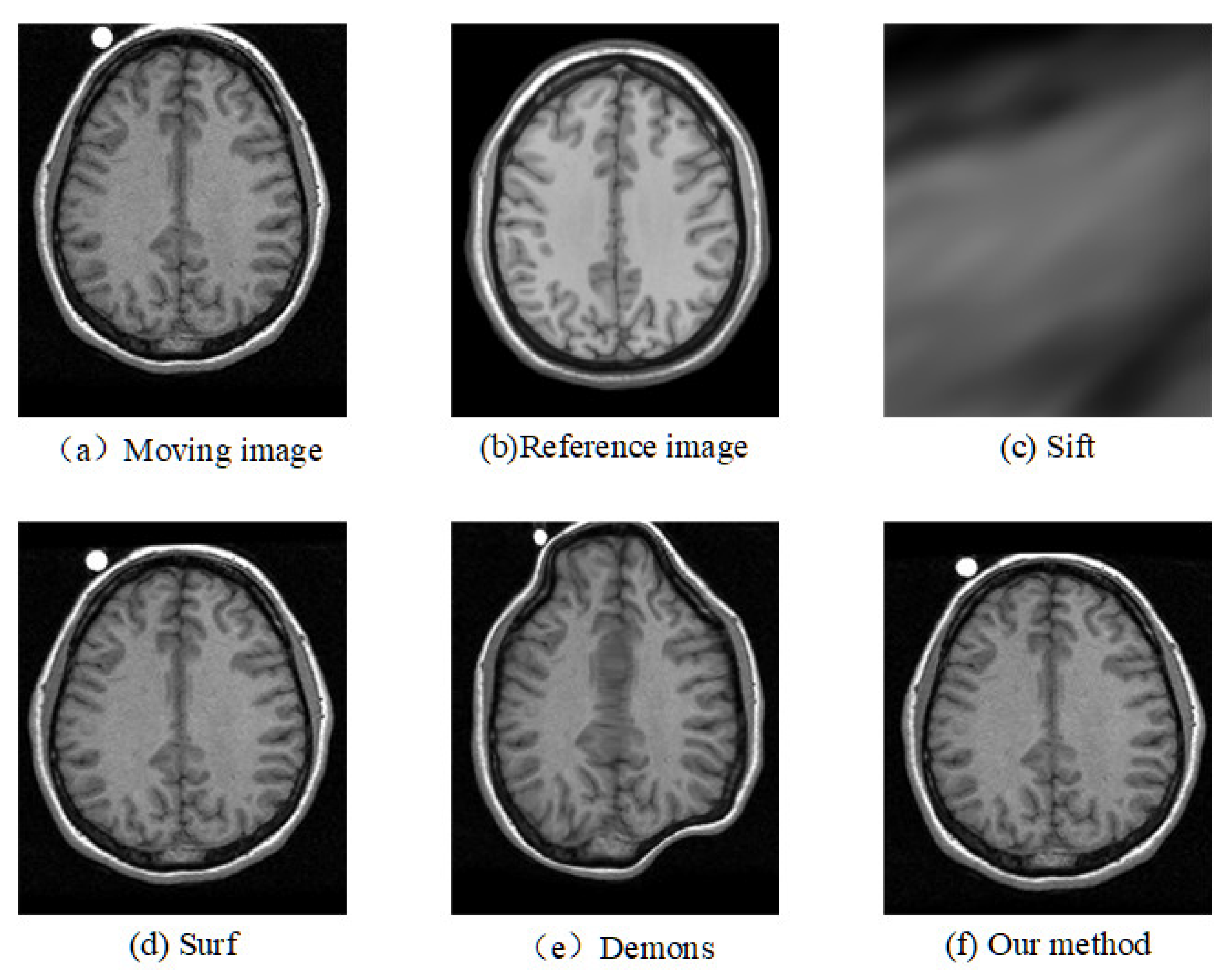
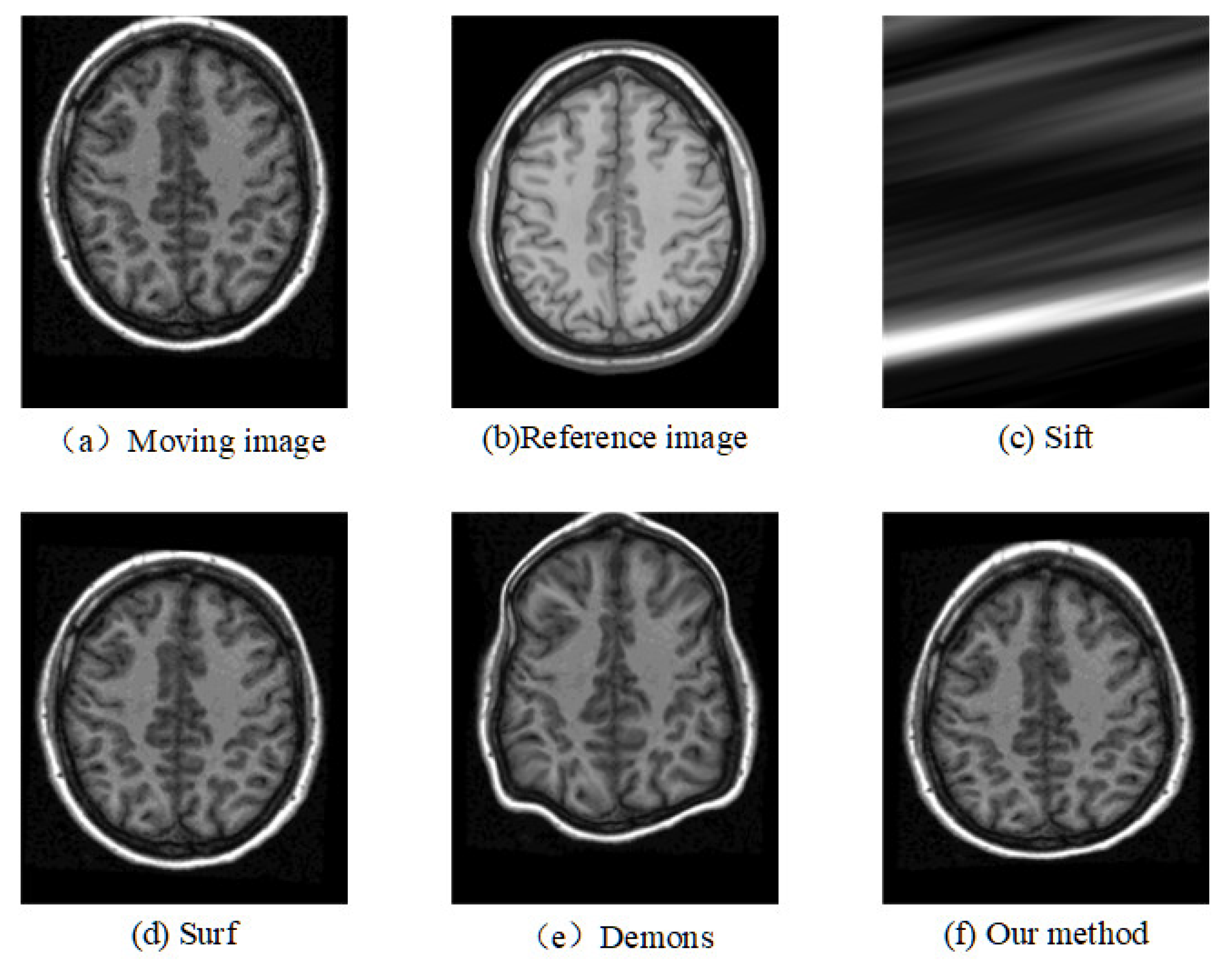
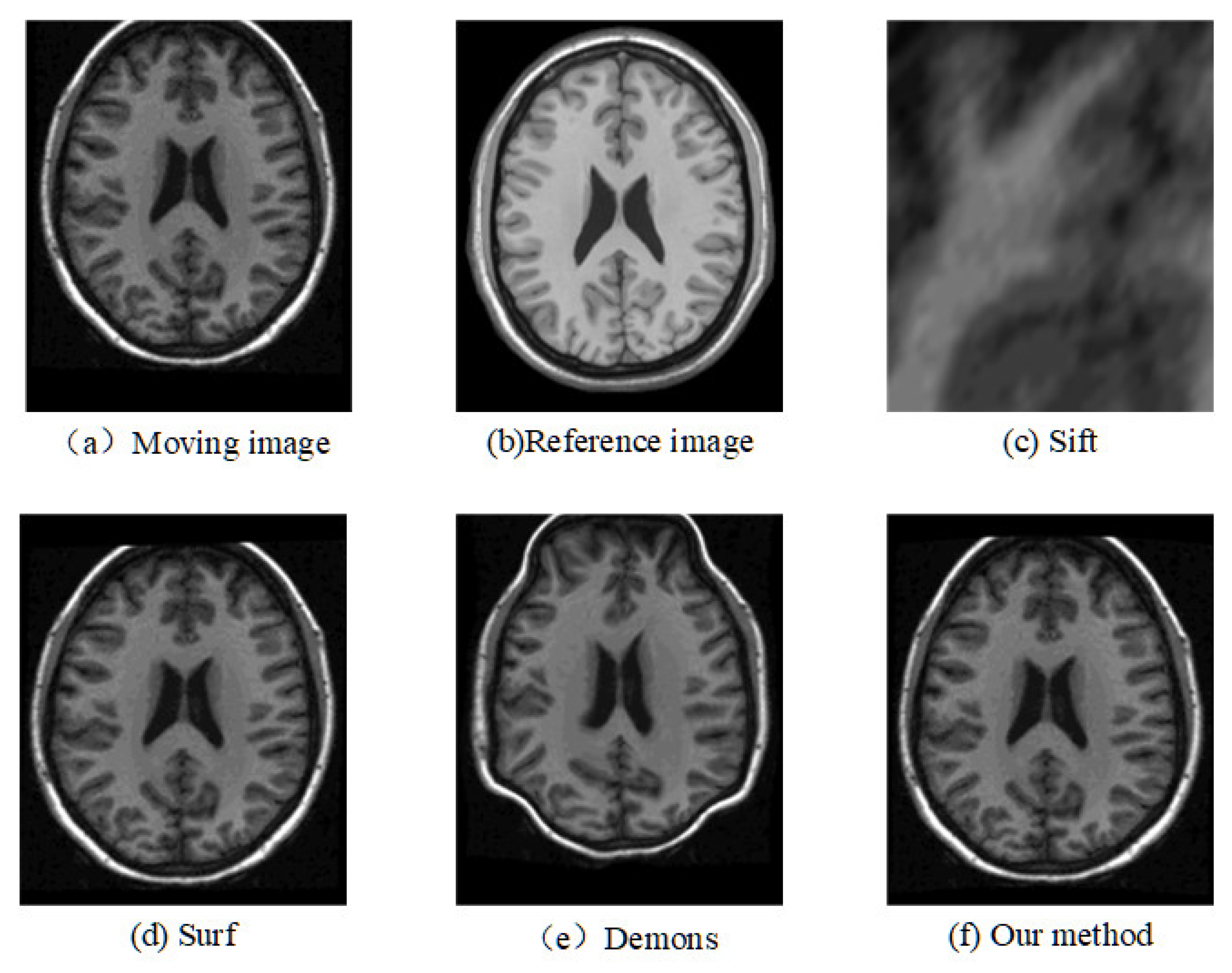
In the study, T1 images from two datasets are used to demonstrate the results of the proposed method, including the CUMC12 dataset from Columbia University Medical Center and the MGH10 dataset from Massachusetts General Hospital [38]. The details of the CUMC12 dataset are as follows: 12 subjects, six males and six females, age range from 26 to 41 years, mean age = 32.7 years, and the acquired T1 image is 256 × 256 × 124 size with image resolution of 0.86 × 0.86 × 1.5 mm³. The details of the MGH10 dataset are as follows: ten subjects, four males and six females, age range from 22 to 29 years, mean age = 25.3 years, and the acquired T1 image was 182 × 218 × 182 size with image resolution of 1 × 1 × 1 mm³. The reference image was selected from the brain ch2 template with an image size of 181 × 217 × 181 and a resolution of 1 × 1 × 1 mm³. To facilitate the next registration, we resample all moving images for maintaining consistency of the size and resolution between the moving images and reference image.

The experimental environment of this work is configured as: Windows10 operating system, Intel(R) Core(TM) i7-8700 CPU @ 3.20GHz processor and 8GB memory. The realization and test of this study are based on the MatlabR2019a.

3. Results

The registration results of the two datasets are shown in

Table 1. Comparison of registration results based on CUMC12 dataset.

Registration Algorithm	Evaluation of Registration Effect (Mean ± Standard Deviation)
	MSD	NCC	NMI	MI
Sift	0.0808 ± 0.0205	0.1083 ± 0.0465	1.0534 ± 0.0024	0.6220 ± 0.0477
Demons	0.0272 ± 0.0037	0.7439 ± 0.0288	1.1228 ± 0.0060	1.3054 ± 0.0738
Surf	0.0337 ± 0.0049	0.7347 ± 0.0345	1.1262 ± 0.0032	1.3478 ± 0.0230
our method	0.0299 ± 0.0048	0.7756 ± 0.0269	1.1309 ± 0.0044	1.3915 ± 0.0233

and

Table 2. Comparison of registration results based on MGH10 dataset.

Registration Algorithm	Evaluation of Registration Effect (Mean ± Standard Deviation)
	MSD	NCC	NMI	MI
Sift	0.0663 ± 0.0123	0.1170 ± 0.0498	1.0557 ± 0.0031	0.6446 ± 0.0568
Demons	0.0271 ± 0.0067	0.7172 ± 0.0145	1.1234 ± 0.0055	1.2892 ± 0.0471
Surf	0.0305 ± 0.0087	0.7137 ± 0.0261	1.1303 ± 0.0031	1.3711 ± 0.0271
our method	0.0245 ± 0.0072	0.7833 ± 0.0287	1.1409 ± 0.0032	1.4708 ± 0.0357

. Moreover, we randomly select two slices based on CUMC12, shown in Figure 6 and Figure 7, and those based on MGH10, shown in Figure 8 and Figure 9.

Table 1 and Table 2 show that the proposed method are better than the Sift, Surf, and Demons algorithms based on four evaluation indexes. The registration results of Sift algorithm are the worst based on MSD, NCC, NMI, and MI. The Demons algorithm is significantly better than the Sift algorithm, but its registration results are not as good as the Surf algorithm. In Table 1, compared with the Demons algorithm, the mean values of NCC, NMI, and MI obtained by the proposed method increased by 0.0317, 0.0081, and 0.0861, respectively. Compared with the Surf algorithm, they increased by 0.0409, 0.0047, and 0.0437, respectively. Moreover, the reduction of MSD is found for our method compared to those for other methods. In Table 2, compared with the Demons algorithm, the mean values of NCC, NMI, and MI obtained by the proposed method increased by 0.0660, 0.0175, and 0.1816, respectively. Compared with the Surf algorithm, they increased by 0.0696, 0.0106, and 0.0997, respectively. Moreover, the reduction of MSD found for our method compared to those for other methods is shown in Table 1 and Table 2.

The corresponding relationship of spatial location can be seen in Figure 6 to Figure 9 between moving image and the reference image. These figures show lots of differences between the moving image and the reference image, including the significant shift of location, different size, the respective concavity and convexity of cerebral cortex, and different degree of smoothness. After registration, the results of our method are the closest to the reference image in multiple aspects, such as spatial location, image size, and brain contour. Surf is second-best, and close to the reference image for the spatial location and size. However, it represented the distortion in the contour of the cerebral cortex to some extent (as shown in Figure 6), and the skewing for some slices (as shown in Figure 8) after registration. The results of the Demons are totally different from the reference image in the spatial location, image size, and contour of the cerebral cortex. It also showed great distortion and deformation. Sift is the worst algorithm, and its current result did not show the brain shape.

4. Discussion

Based on the CUMC12 and MGH10 datasets, this study performed a comparison of four registration techniques and found that: (1) Sift is the worst registration for the T1 brain image; (2) Demons is better than Sift for the registration results, but it shows obvious distortion and deformation; (3) the Surf algorithm has significant advantages compared to the Sift and Demons algorithms, but there is still some distortion and skewing; (4) compared with the Surf, Demons, and Sift algorithms, the proposed method in the study not only has the best performance in four types of quantitative indexes (MSD, NCC, NMI, and MI), but also shows the best results for visualization of brain image after registration, mainly in the spatial location, brain size, contour of cerebral cortex, and some registration details.

The Sift algorithm first finds feature points on different scale paces and feature vector containing position, scale, and orientation for the image registration [39,40,41]. The Sift algorithm can filter out low-contrast points during its execution [42], and thus it may not detect valid feature points for the relatively smooth brain images, leading to an increase in the false matching rate. In this study, the low contrast of different individual brain images may cause fewer effective feature points to be detected, and the feature vector during the registration is unduly dependent on the principal direction of the feature points. Therefore, a slight shift in the principal direction may lead to many errors during the matching of feature point. The above description may be the reason for the significant distortion after the registration of the Sift algorithm in this paper.

The Demons algorithm determines the transformation parameters by internal and external aspects. The internal aspect is the gradient of the reference image, whereas the external aspect is the gray-level difference between the reference image and moving image. The pixel motion is driven by the gradient and the gray-level difference, which can make the image to be aligned closer to the reference image [42,43,44]. Therefore, the great difference between the two images may cause a huge deformation due to the significant gradient and gray-level difference, leading to the damage of normal brain anatomy [27,45]. Different individuals may vary significantly in size, morphological contours, and tissue details for the brain, so the Demons algorithm may be unsuitable for spatial registration of different individuals.

The Surf algorithm carried out the registration based on the extraction of feature points [46]. Previous studies found that fewer features may obtain higher matching accuracy, whereas more features may often cause an increase in error matching of feature points. Therefore, the Surf algorithm extracts a limited number of feature points for ensuring the registration effect [42]. The Surf algorithm usually extracts only a few feature points at the brain boundaries during the registration of brain images, which cannot cover the key points of spatial location within different brain tissues. Therefore, these may lead to unsatisfactory spatial consistency in the current study.

The method in this paper can extract features points from not only the contour of the cerebral cortex but also the boundary of the internal brain tissues, which consider not only the morphology of the brain but also the critical locations inside the brain tissues during registration. To avoid the problem of more incorrect matching pairs caused by the inclusion of too many feature points, the RANSAC algorithm is also used to eliminate the incorrect matching pairs as much as possible, ensuring the correctness of the transformation parameters during registration. Therefore, the proposed method can guarantee the correspondence of different individual brain images for spatial location and anatomical structure as much as possible. According to the steps of our technique, the proposed method is of the same time complexity as the surf algorithm.

In summary, we fully considered the differences and complexity of human brain structures during the registration, achieving the accurate registration of different individual brain images. However, there are still some weaknesses in this study. First, there are relatively fewer brain images in the current study, and thus the registration effect of the proposed method still needs a large number of brain images for validation. Second, this work is carried out based on only brain T1 image. Third, all steps of this registration process may be further optimized. For example, the method of brain segmentation may be replaced by machine learning or deep learning method (such as U-Net). In the future, we will further improve the method, and also try to apply the proposed method to other brain images (such as T2 and CT) for higher universality.

5. Conclusions

This paper proposed a new technique for brain image registration, which will be valuable for brain image reconstruction, fusion, and statistical comparison analyses.

References

1. Sergent, J. Brain-imaging studies of cognitive functions. Trends Neurosci. 1994, 17, 221–227. [Google Scholar] [CrossRef] [PubMed]
2. Andrade, N.; Faria, F.A.; Cappabianco, F.A.M. A practical review on medical image registration: From rigid to deep learning based approaches. In Proceedings of the 2018 31st SIBGRAPI Conference on Graphics, Patterns and Images (SIBGRAPI), Paraná, Brazil, 29 October–1 November 2018. [Google Scholar]
3. Hermessi, H.; Mourali, O.; Zagrouba, E. Multimodal medical image fusion review: Theoretical background and recent advances. Signal Process. 2021, 183, 108036. [Google Scholar] [CrossRef]
4. Zhangpei, C. Research on 3D Biomedical Brain Image Registration Algorithm Based on Deep Learning. Master’s Thesis, Anhui University, Hefei, China, 2020. [Google Scholar]
5. Kuppala, K.; Banda, S.; Barige, T.R.; Fusion, D. An overview of deep learning methods for image registration with focus on feature-based approaches. Int. J. Image Data Fusion 2020, 11, 113–135. [Google Scholar] [CrossRef]
6. Yuen, J.; Barber, J.; Ralston, A.; Gray, A.; Walker, A.; Hardcastle, N.; Schmidt, L.; Harrison, K.; Poder, J.; Sykes, J.R. An international survey on the clinical use of rigid and deformable image registration in radiotherapy. J. Appl. Clin. Med. Phys. 2020, 21, 10–24. [Google Scholar] [CrossRef] [PubMed]
7. Presti, L.L.; La Cascia, M. Multi-modal Medical Image Registration by Local Affine Transformations. In Proceedings of the ICPRAM, Funchal, Portugal, 16–18 January 2018. [Google Scholar]
8. Haskins, G.; Kruger, U.; Yan, P. Deep learning in medical image registration: A survey. Mach. Vis. Appl. 2020, 31, 8. [Google Scholar] [CrossRef]
9. Zachariadis, O.; Teatini, A.; Satpute, N.; Gómez-Luna, J.; Mutlu, O.; Elle, O.J.; Olivares, J. Accelerating B-spline interpolation on GPUs: Application to medical image registration. Comput. Methods Programs Biomed. 2020, 193, 105431. [Google Scholar] [CrossRef]
10. Thirion, J.P. Image matching as a diffusion process: An analogy with Maxwell’s demons. Med. Image Anal. 1998, 2, 221–227. [Google Scholar] [CrossRef]
11. Balakrishnan, G.; Zhao, A.; Sabuncu, M.R.; Guttag, J.; Dalca, A.V. An unsupervised learning model for deformable medical image registration. In Proceedings of the IEEE Conference on Computer Vision and pattern recognition, Salt Lake City, UT, USA, 18–23 June 2018. [Google Scholar]
12. Lowe, D.G. Object recognition from local scale-invariant features. Int. J. Comput. Vis. 2004, 60, 91–110. [Google Scholar] [CrossRef]
13. Bay, H.; Tuytelaars, T.; Gool, L.V. Surf: Speeded up robust features. In Proceedings of the European Conference on Computer Vision, Berlin/Heidelberg, Germany, 7–13 May 2006. [Google Scholar]
14. Harris, C.; Stephens, M. A combined corner and edge detector. In Proceedings of the Alvey Vision Conference, Manchester, UK, 31 August–2 September 1988. [Google Scholar]
15. Fu, Y.; Lei, Y.; Wang, T.; Curran, W.J.; Liu, T.; Yang, X. Deep learning in medical image registration: A review. Phys. Med. Biol. 2020, 65, 20TR01. [Google Scholar] [CrossRef]
16. Abbasi, S.; Tavakoli, M.; Boveiri, H.R.; Shirazi, M.A.M.; Khayami, R.; Khorasani, H.; Javidan, R.; Mehdizadeh, A. Medical image registration using unsupervised deep neural network: A scoping literature review. Biomed. Signal. Process. Control. 2022, 73, 103444. [Google Scholar] [CrossRef]
17. Fan, J.; Cao, X.; Yap, P.-T.; Shen, D. BIRNet: Brain image registration using dual-supervised fully convolutional networks. Med. Image Anal. 2019, 54, 193–206. [Google Scholar] [CrossRef]
18. Mahapatra, D.; Ge, Z. Training data independent image registration using generative adversarial networks and domain adaptation. Pattern. Recognit. 2020, 100, 107109. [Google Scholar] [CrossRef]
19. Chen, J.; He, Y.; Frey, E.C.; Li, Y.; Du, Y. Vit-v-net: Vision transformer for unsupervised volumetric medical image registration. arXiv 2021, arXiv:2104.06468. [Google Scholar]
20. Song, L.; Liu, G.; Ma, M. TD-Net: Unsupervised medical image registration network based on Transformer and CNN. Appl. Intell. 2022, 52, 18201–18209. [Google Scholar] [CrossRef]
21. Fischler, M.A.; Bolles, R.C. Random sample consensus: A paradigm for model fitting with applications to image analysis and automated cartography. Commun. ACM 1981, 24, 381–395. [Google Scholar] [CrossRef]
22. Jiying, L.; Yonghong, Y.; Qiang, W.; Yan, W.; Yilin, Y. Research on Improved SURF Breast Registration Algorithm in Multi-Mode MRI. Laser Optoelectron. Pro 2020, 57, 121010. [Google Scholar] [CrossRef]
23. Bishop, C.M.; Nasrabadi, N.M. Pattern Recognition and Machine Learning, 1st ed.; Springer: Berlin, Germany, 2006; pp. 78–110. [Google Scholar]
24. Yongxia, L. Research on Thickness Measurement and Registration of Cerebral Cortex Based on MRI. Master’s Thesis, Liaoning University, Shenyang, China, 2021. [Google Scholar]
25. Dempster, A.P.; Laird, N.M.; Rubin, D.B. Maximum likelihood from incomplete data via the EM algorithm. J. R. Stat. Soc. Ser. B 1977, 39, 1–22. [Google Scholar]
26. Öziç, M.Ü.; Ekmekci, A.H.; Özşen, S. Atlas-Based Segmentation Pipelines on 3D Brain MR Images: A Preliminary Study. BRAIN. Broad Res. Artif. Intell. Neurosci. 2018, 9, 129–140. [Google Scholar]
27. Derong, Y. Research on Non-Rigid Medical Image Registration Technology. Master’s Thesis, Nanchang Hangkong University, Nanchang, China, 2019. [Google Scholar]
28. Zitova, B.; Flusser, J. Image registration methods: A survey. Image Vis. Comput. 2003, 21, 977–1000. [Google Scholar] [CrossRef]
29. Sarvaiya, J.N.; Patnaik, S.; Bombaywala, S. Image registration by template matching using normalized cross-correlation. In Proceedings of the 2009 International Conference on Advances in Computing Control, and Telecommunication Technologies, Angalore, India, 28–29 December 2009. [Google Scholar]
30. Studholme, C.; Hill, D.L.; Hawkes, D.J. An overlap invariant entropy measure of 3D medical image alignment. Pattern Recognit. 1999, 32, 71–86. [Google Scholar] [CrossRef]
31. Viola, P.; Wells, W.M., III. Alignment by maximization of mutual information. Int. J. Comput. Vis. 1997, 24, 137–154. [Google Scholar] [CrossRef]
32. Fu, Y.; Wang, T.; Lei, Y.; Patel, P.; Jani, A.B.; Curran, W.J.; Liu, T.; Yang, X. Deformable MR-CBCT prostate registration using biomechanically constrained deep learning networks. Med. Phys. 2021, 48, 253–263. [Google Scholar] [CrossRef] [PubMed]
33. Liu, S.; Yang, B.; Wang, Y.; Tian, J.; Yin, L.; Zheng, W. 2D/3D multimode medical image registration based on normalized cross-correlation. Appl. Sci. 2022, 12, 2828. [Google Scholar] [CrossRef]
34. Gerber, N.; Carrillo, F.; Abegg, D.; Sutter, R.; Zheng, G.; Fürnstahl, P. Evaluation of CT-MR image registration methodologies for 3D preoperative planning of forearm surgeries. J. Orthop. Res. 2020, 38, 1920–1930. [Google Scholar] [CrossRef] [PubMed]
35. Chen, Y.; He, F.; Li, H.; Zhang, D.; Wu, Y. A full migration BBO algorithm with enhanced population quality bounds for multimodal biomedical image registration. Appl. Soft. Comput. 2020, 93, 106335. [Google Scholar] [CrossRef]
36. Paul, S.; Pati, U.C. High-resolution optical-to-SAR image registration using mutual information and SPSA optimisation. IET Image Process 2021, 15, 1319–1331. [Google Scholar] [CrossRef]
37. Nan, A.; Tennant, M.; Rubin, U.; Ray, N. Drmime: Differentiable mutual information and matrix exponential for multi-resolution image registration. In Proceedings of the Medical Imaging with Deep Learning, Montreal, QC, Canada, 6–9 July 2020. [Google Scholar]
38. Klein, A.; Andersson, J.; Ardekani, B.A.; Ashburner, J.; Avants, B.; Chiang, M.-C.; Christensen, G.E.; Collins, D.L.; Gee, J.; Hellier, P. Evaluation of 14 nonlinear deformation algorithms applied to human brain MRI registration. Neuroimage 2009, 46, 786–802. [Google Scholar] [CrossRef]
39. Bian, J.-W.; Wu, Y.-H.; Zhao, J.; Liu, Y.; Zhang, L.; Cheng, M.-M.; Reid, I. An evaluation of feature matchers for fundamental matrix estimation. In Proceedings of the British Machine Vision Conference (BMVC), Cardiff, UK, 9—12 September 2019. [Google Scholar]
40. Zhang, T.; Zhao, R.; Chen, Z. Application of migration image registration algorithm based on improved SURF in remote sensing image mosaic. IEEE Access 2020, 8, 163637–163645. [Google Scholar] [CrossRef]
41. Chen, S.; Zhong, S.; Xue, B.; Li, X.; Zhao, L.; Chang, C.-I. Iterative scale-invariant feature transform for remote sensing image registration. IEEE Trans. Geosci. Remote Sens. 2020, 59, 3244–3265. [Google Scholar] [CrossRef]
42. Damas, S.; Cordón, O.; Santamaría, J. Medical image registration using evolutionary computation: An experimental survey. IEEE Comput. Intell. Mag. 2011, 6, 26–42. [Google Scholar] [CrossRef]
43. Lan, S.; Guo, Z.; You, J. Non-rigid medical image registration using image field in Demons algorithm. Pattern Recognit. Lett. 2019, 125, 98–104. [Google Scholar] [CrossRef]
44. Chakraborty, S.; Pradhan, R.; Ashour, A.S.; Moraru, L.; Dey, N. Grey-Wolf-Based Wang’s Demons for retinal image registration. Entropy 2020, 22, 659. [Google Scholar] [CrossRef]
45. Han, R.; De Silva, T.; Ketcha, M.; Uneri, A.; Siewerdsen, J. A momentum-based diffeomorphic demons framework for deformable MR-CT image registration. Phys. Med. Biol. 2018, 63, 215006. [Google Scholar] [CrossRef]
46. Mancini, M.; Casamitjana, A.; Peter, L.; Robinson, E.; Crampsie, S.; Thomas, D.L.; Holton, J.L.; Jaunmuktane, Z.; Iglesias, J.E. A multimodal computational pipeline for 3D histology of the human brain. Sci. Rep. 2020, 10, 13839. [Google Scholar] [CrossRef]
Figure 1. Flow chart of the proposed method.
Electronics 12 00738 g001
Figure 2. Segmentation of brain tissue.
Electronics 12 00738 g002
Figure 3. Edge detection of brain tissues.
Electronics 12 00738 g003
Figure 4. Matching results of feature points.
Electronics 12 00738 g004
Figure 5. Remaining matching pairs of feature points.
Electronics 12 00738 g005
Figure 6. Registration results of any one slice from any T1 image based on CUMC12 dataset.
Electronics 12 00738 g006
Figure 7. Registration results of another slice from another T1 image based on CUMC12 dataset.
Electronics 12 00738 g007
Figure 8. Registration results of any one slice from any T1 image based on MGH10 dataset.
Electronics 12 00738 g008
Figure 9. Registration results of another slice from another T1 image based on MGH10 dataset.
Electronics 12 00738 g009