
Automated Pre-Play Analysis of American Football Formations Using Deep Learning

Abstract
:1. Introduction
1.1. Related Work
1.2. Scope of Work
2. American Football
3. Methods
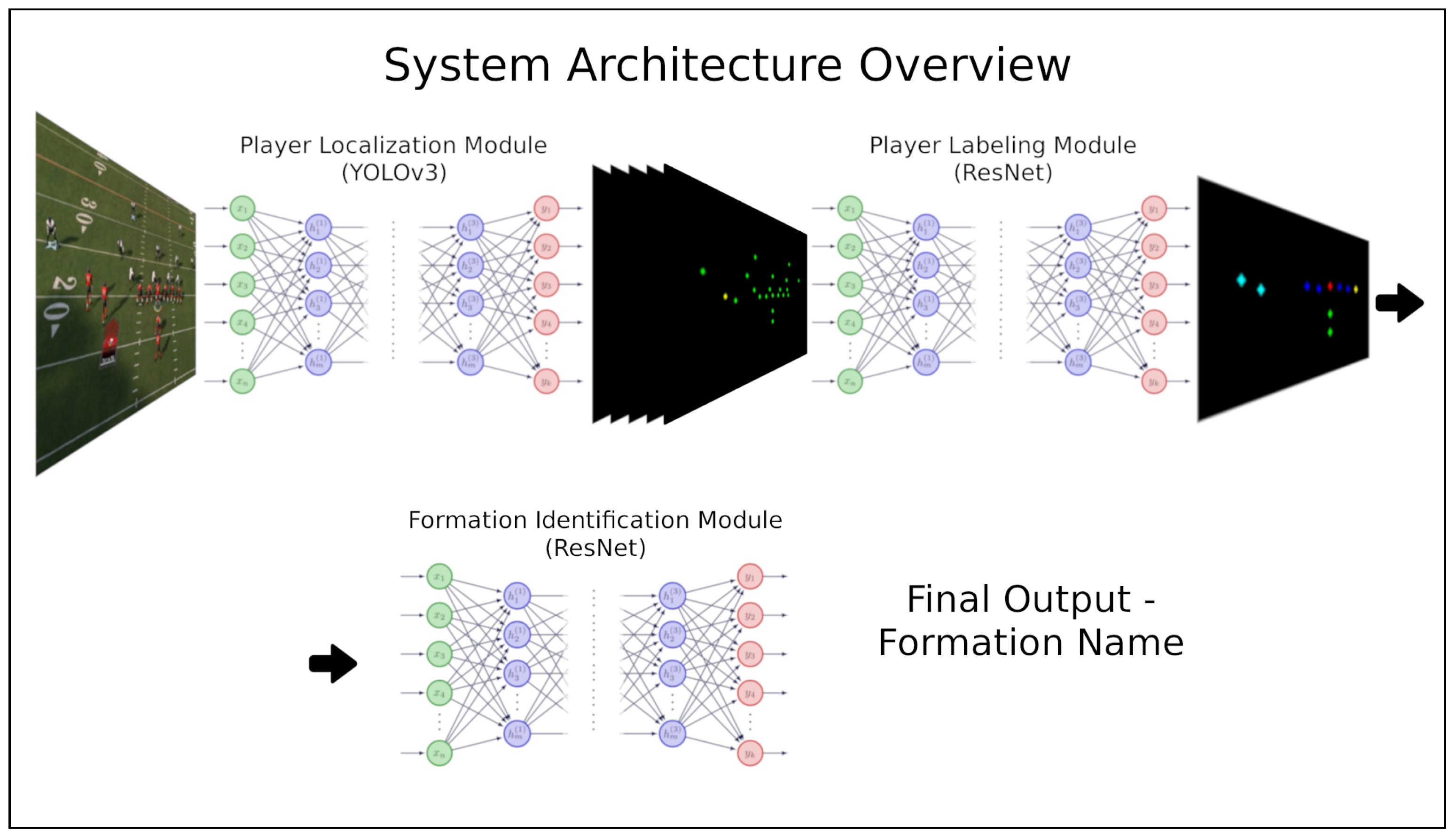
3.1. System Modules
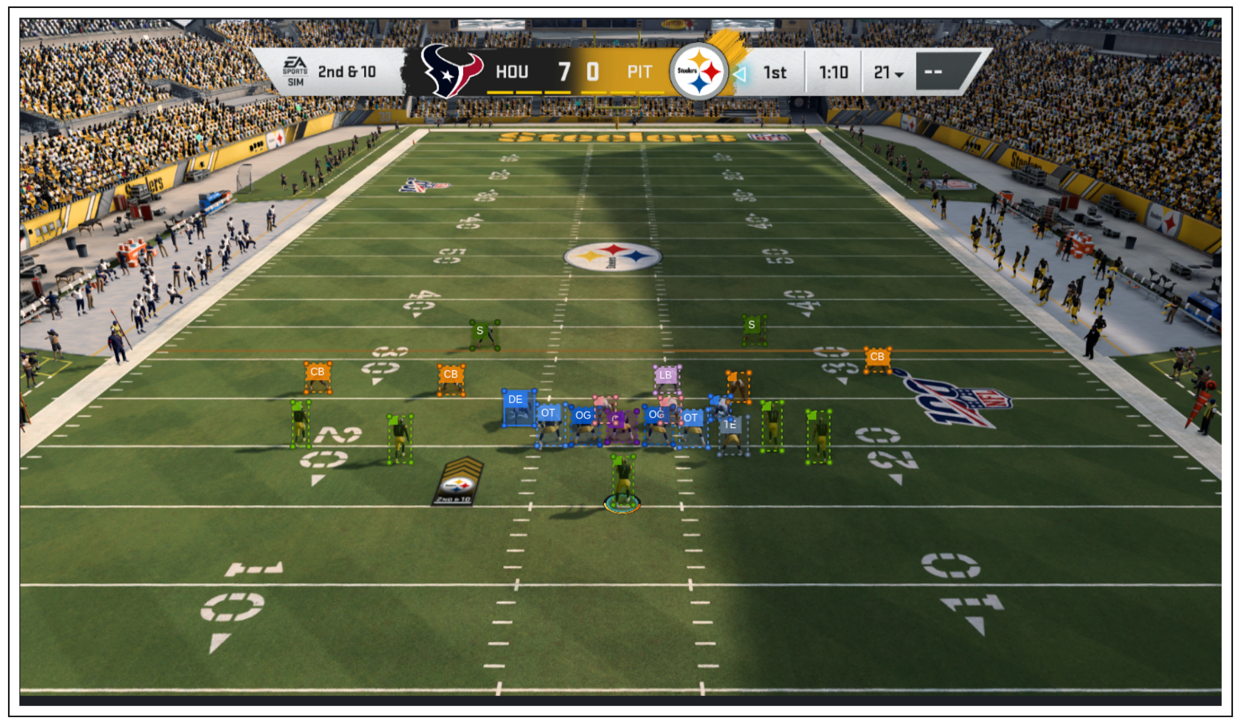
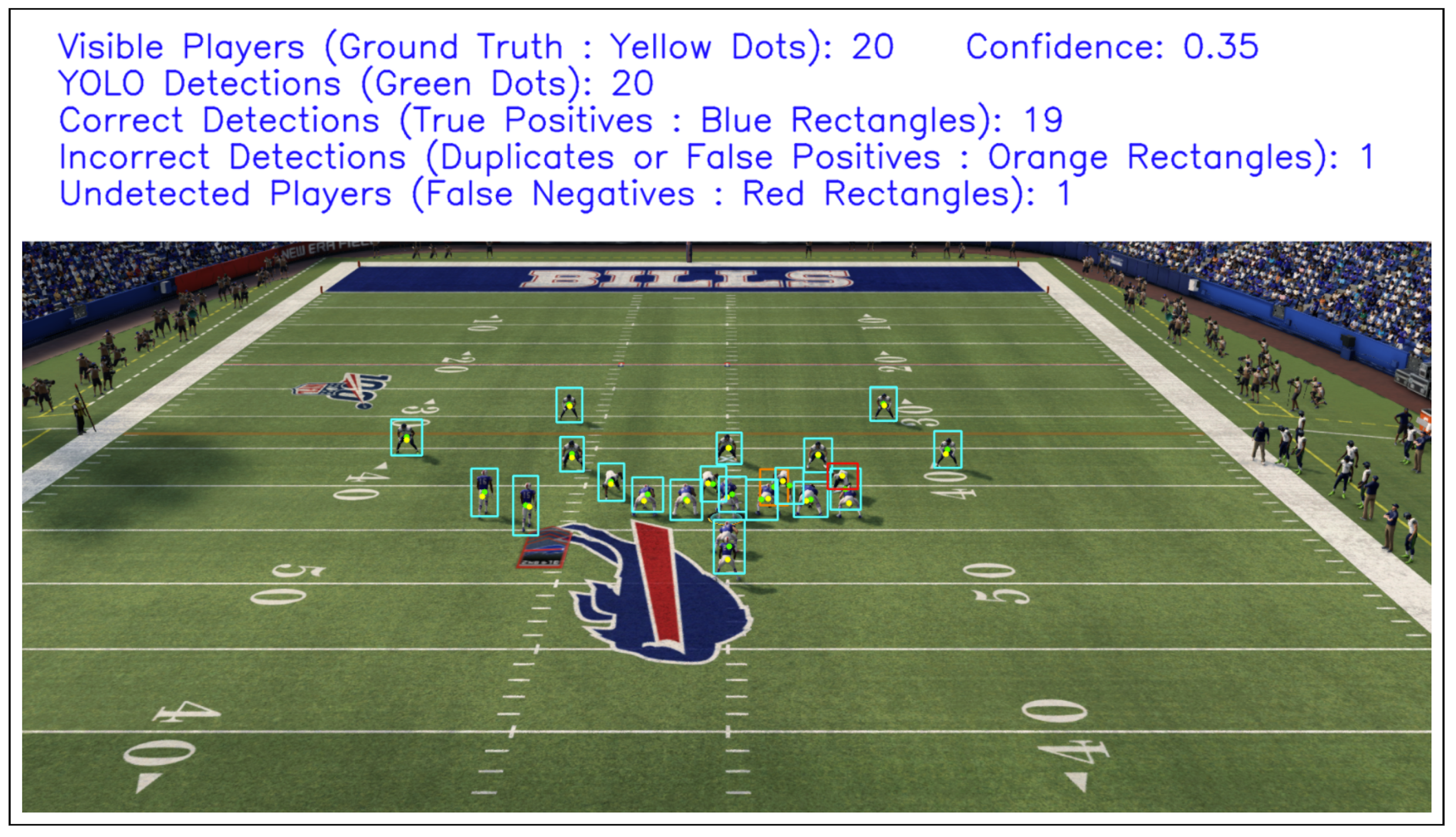
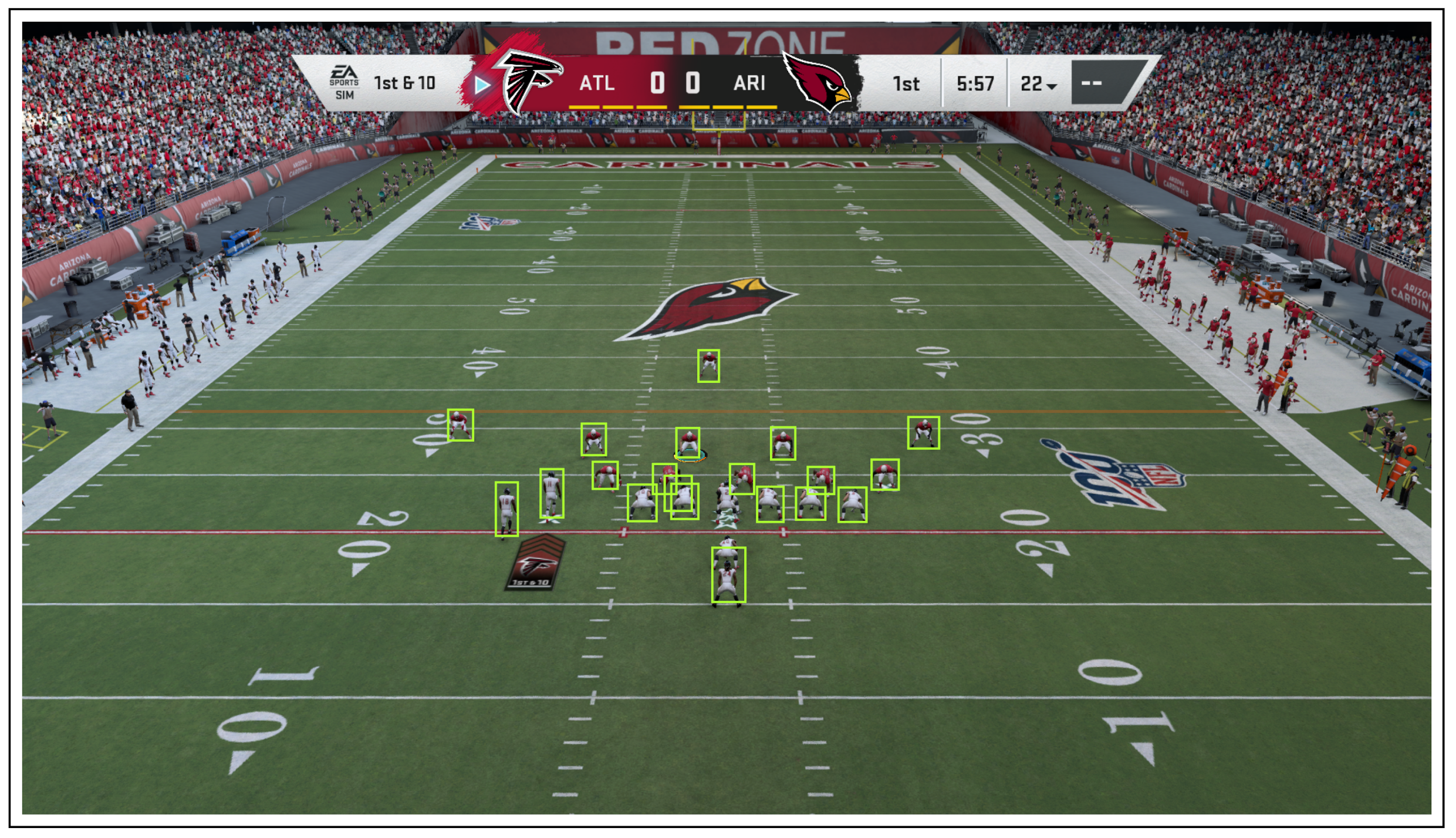
3.1.1. YOLO: Player Localization Module
3.1.2. ResNet: Player-Labeling Module
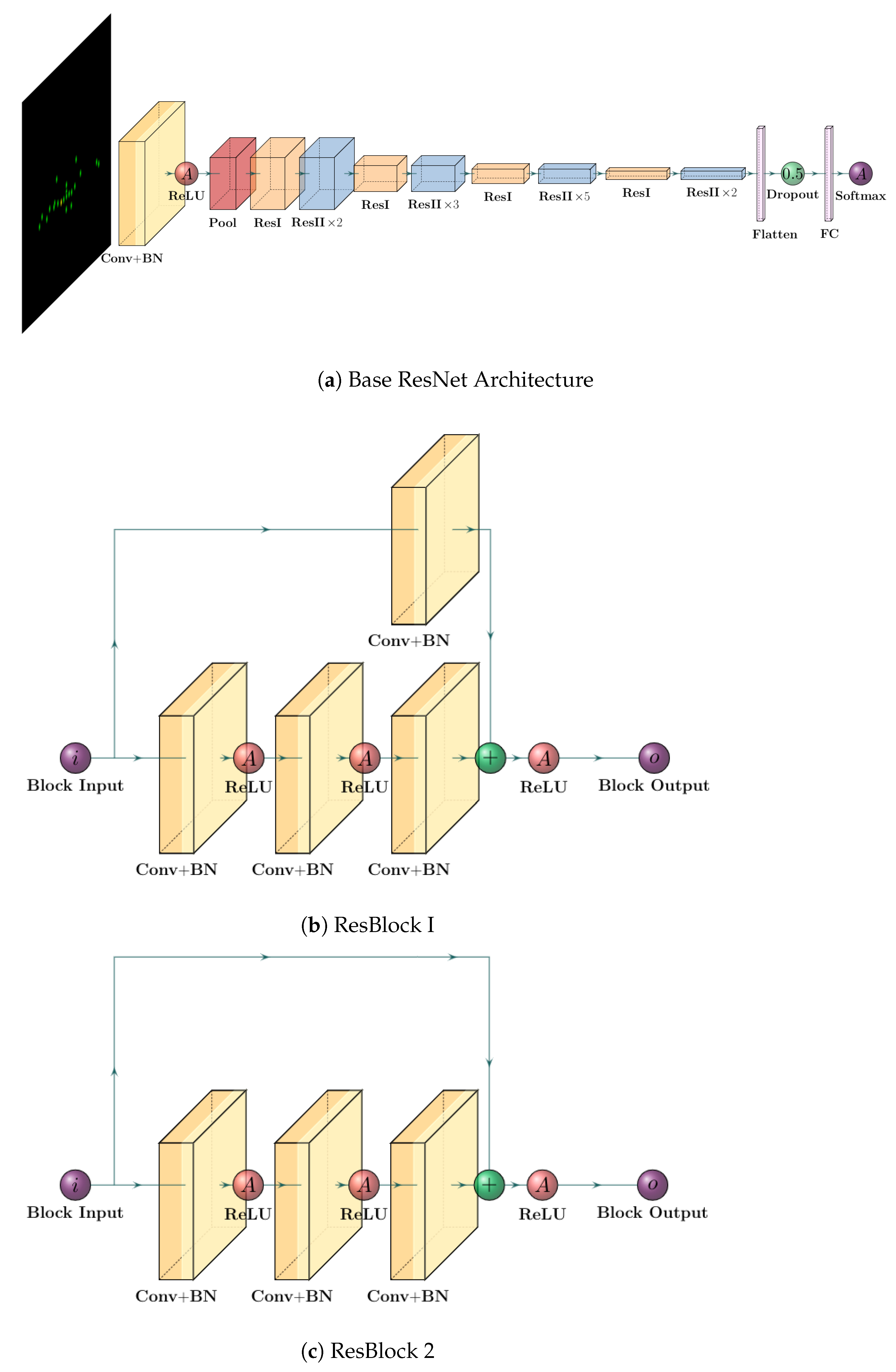
3.1.3. ResNet: Formation Identification Module
3.2. Input Representations
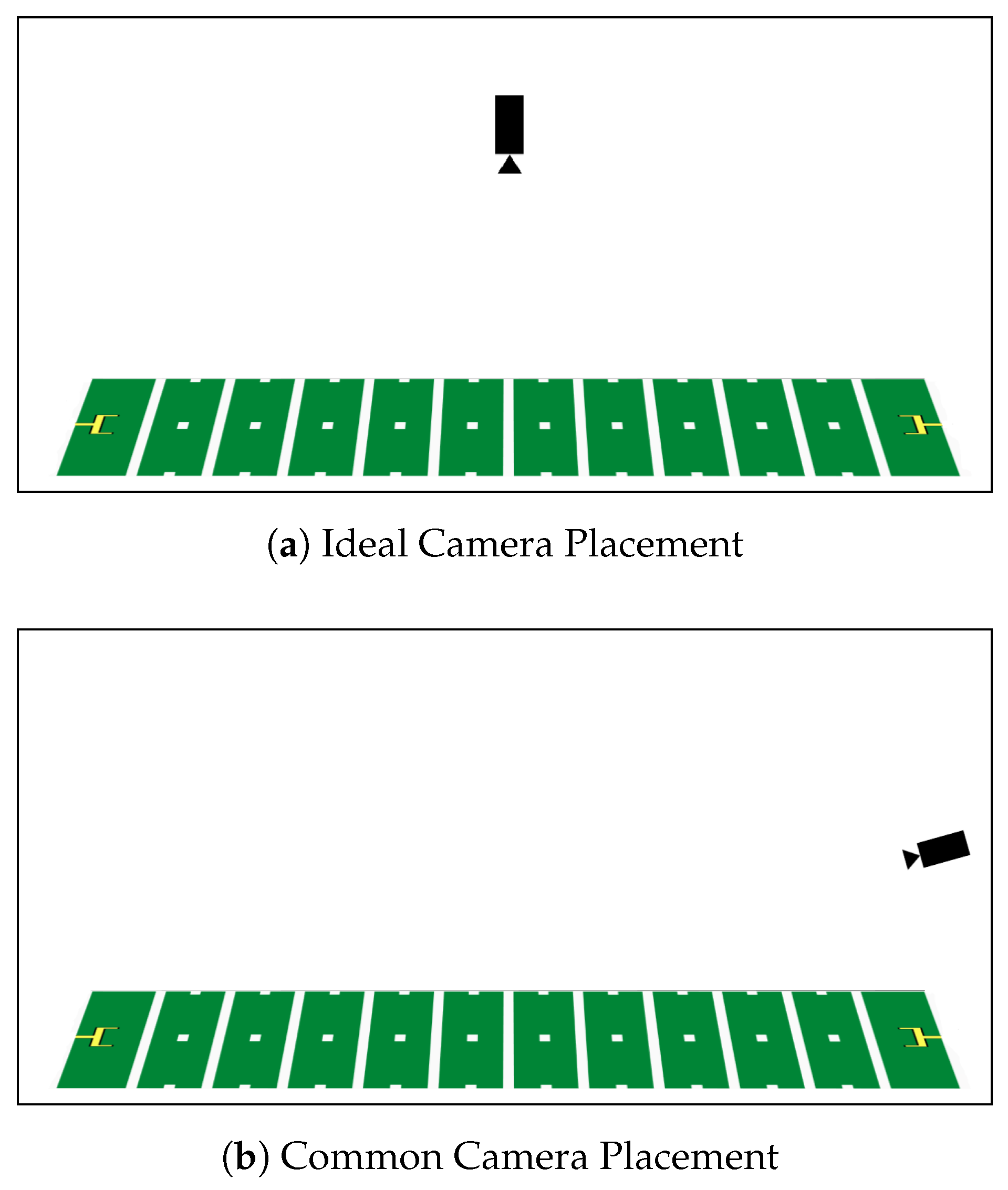
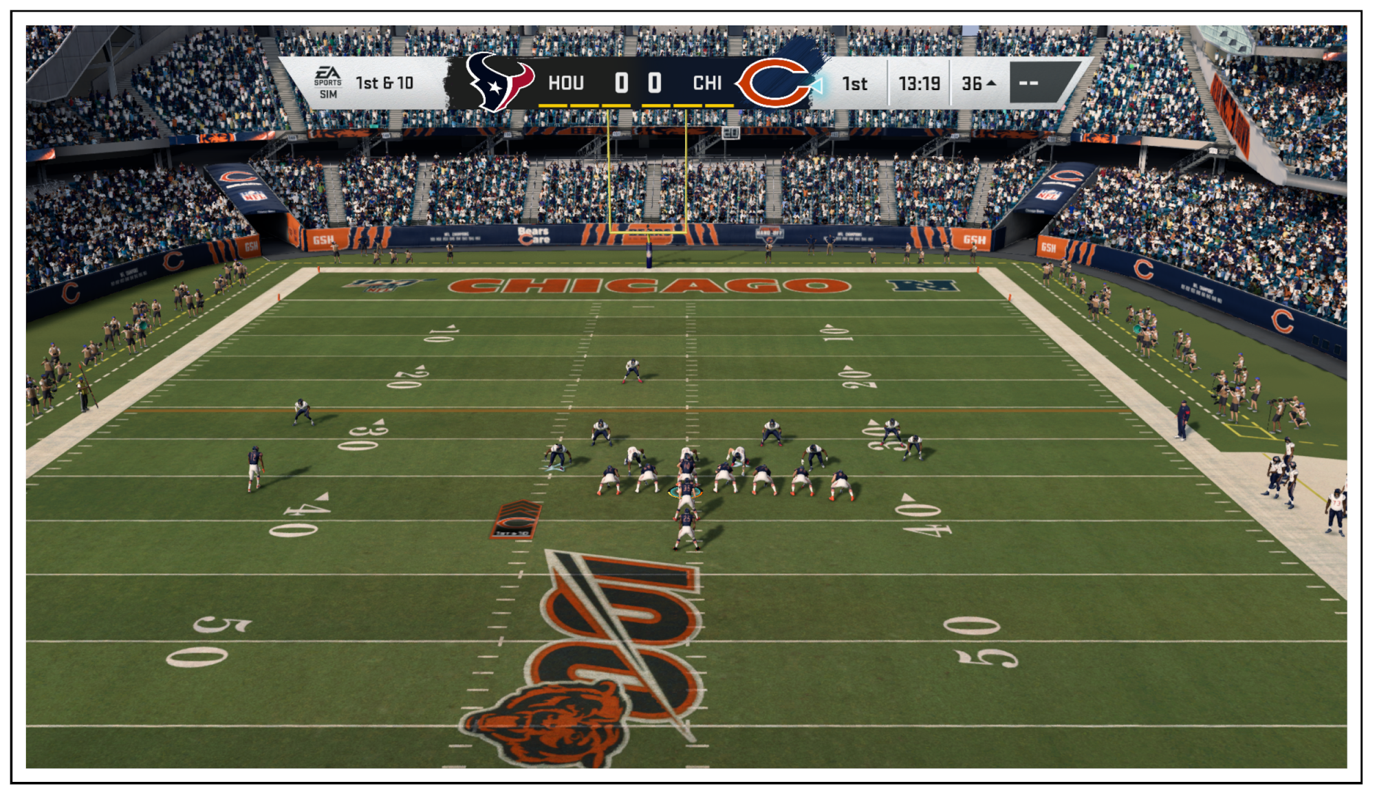
3.2.1. Input to the Player Localization Module
3.2.2. Input to the Player-Labeling Module
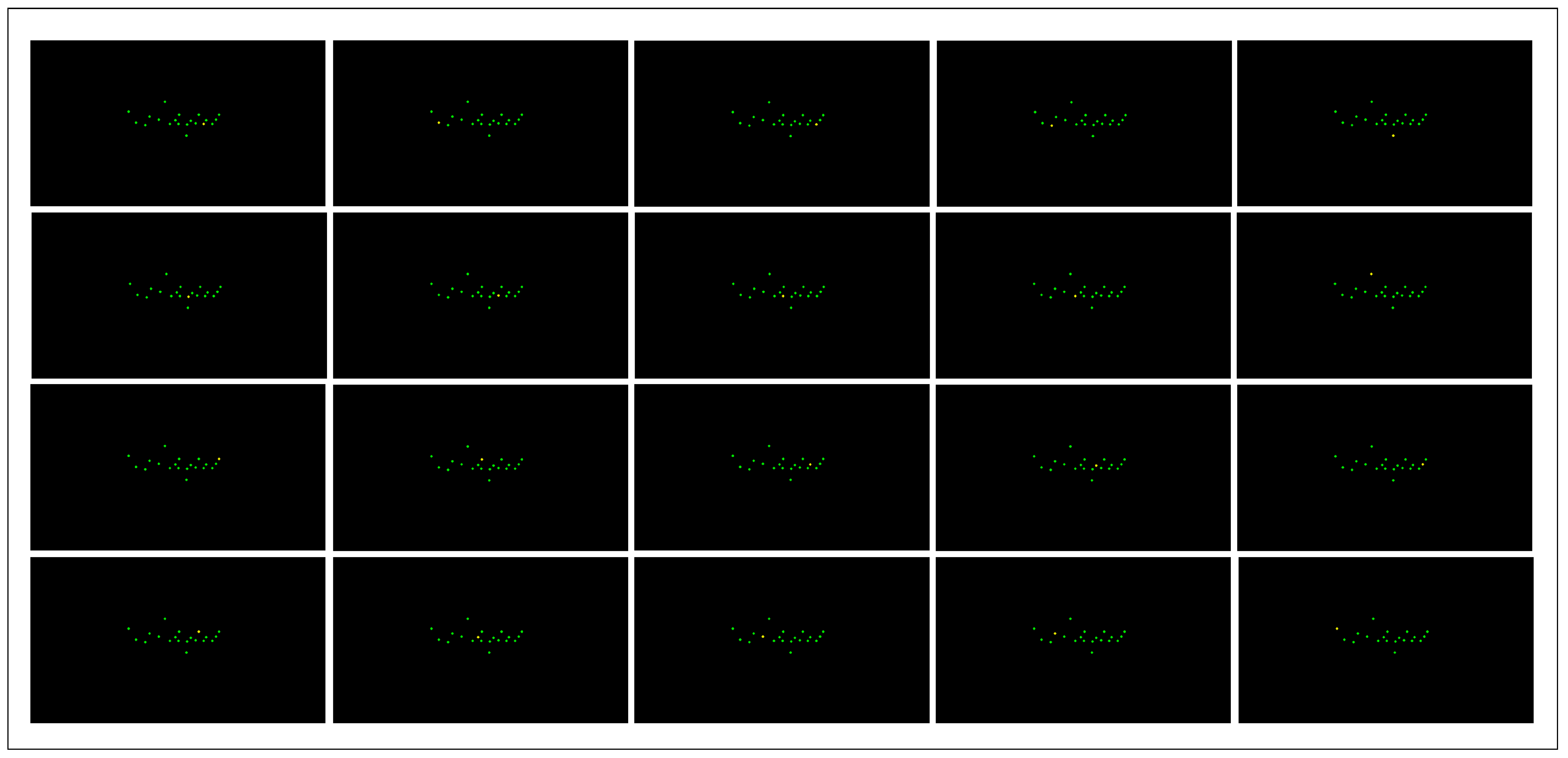
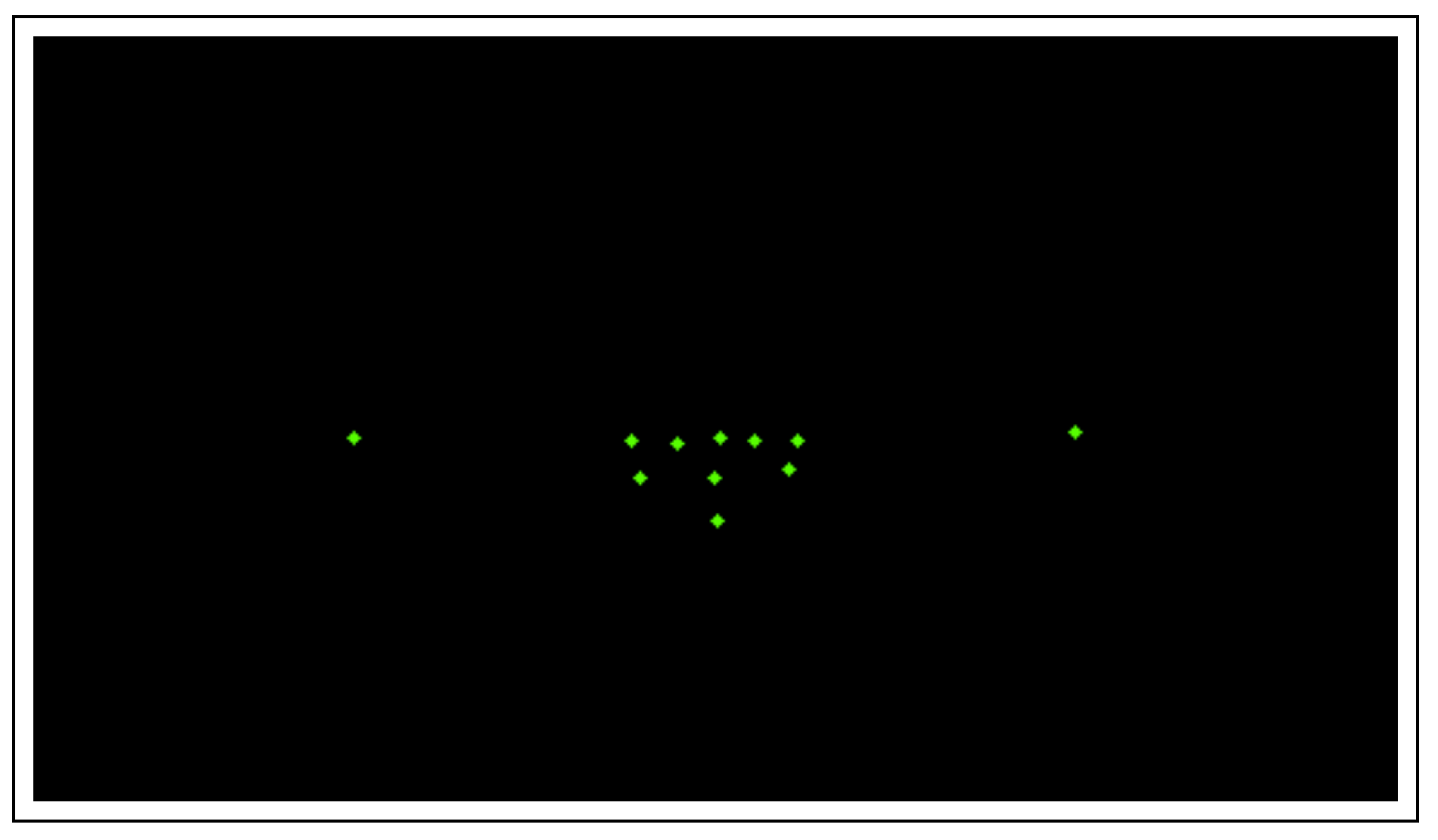
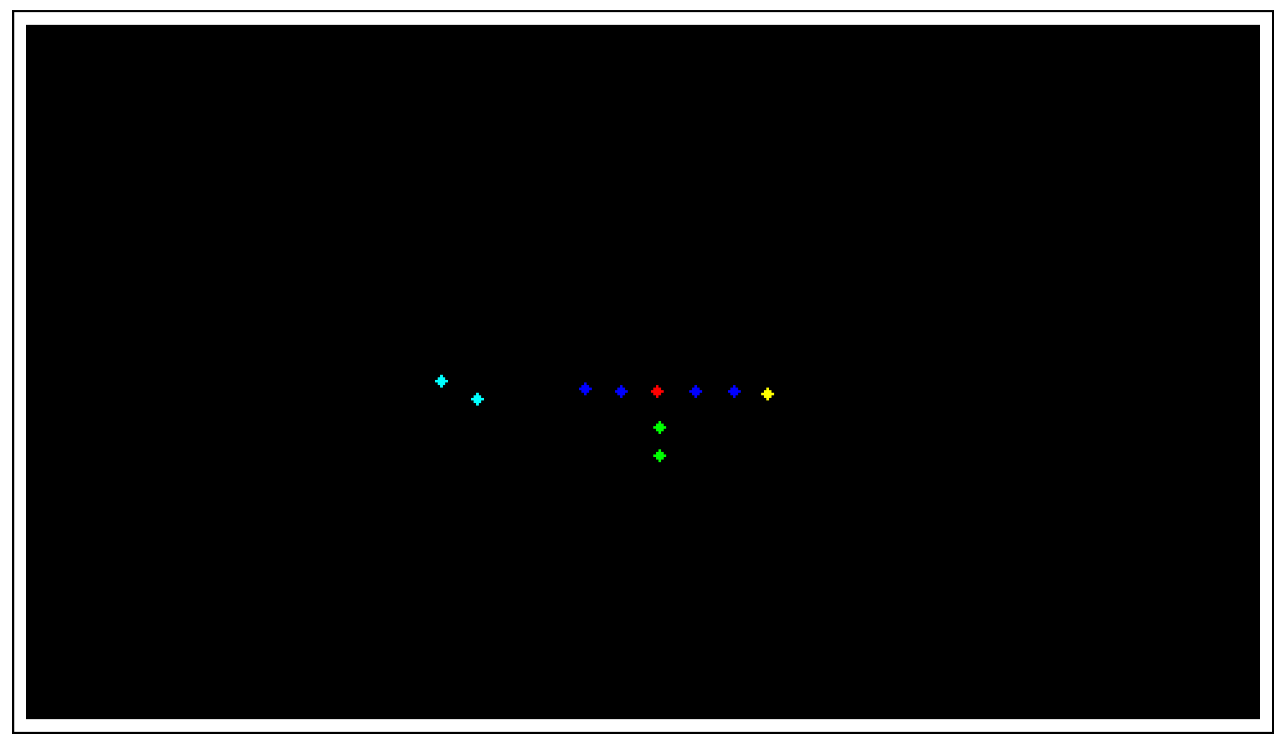
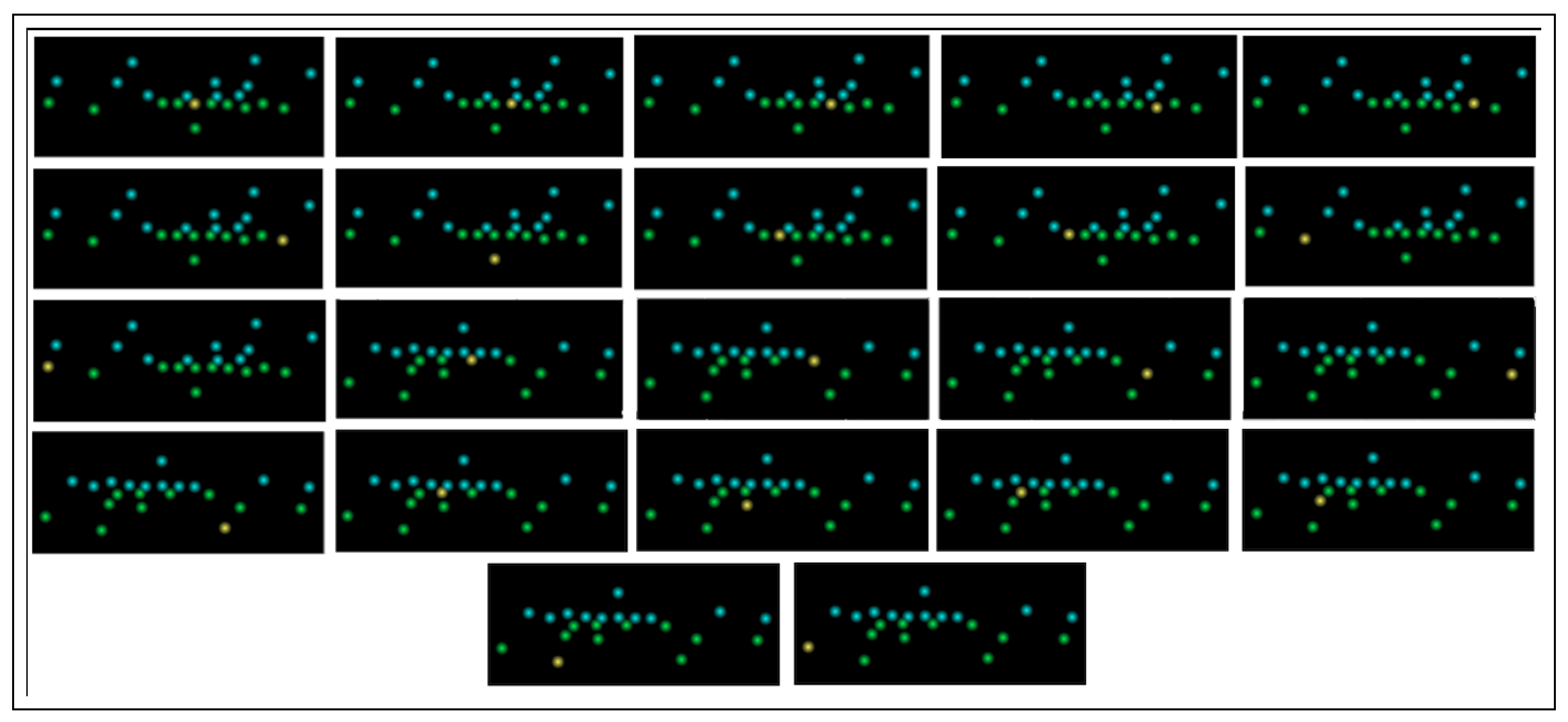
3.2.3. Input to the Formation Identification Module
4. Experiments
4.1. Dataset
4.2. Data Augmentation
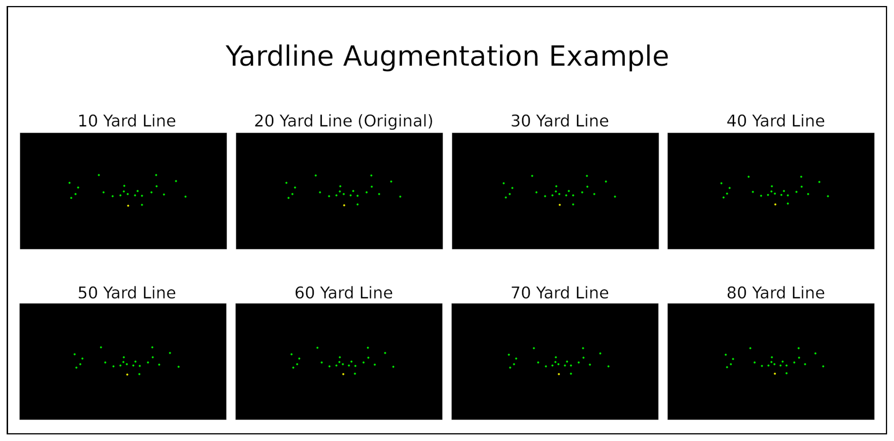
4.2.1. Yard Line Data Augmentation
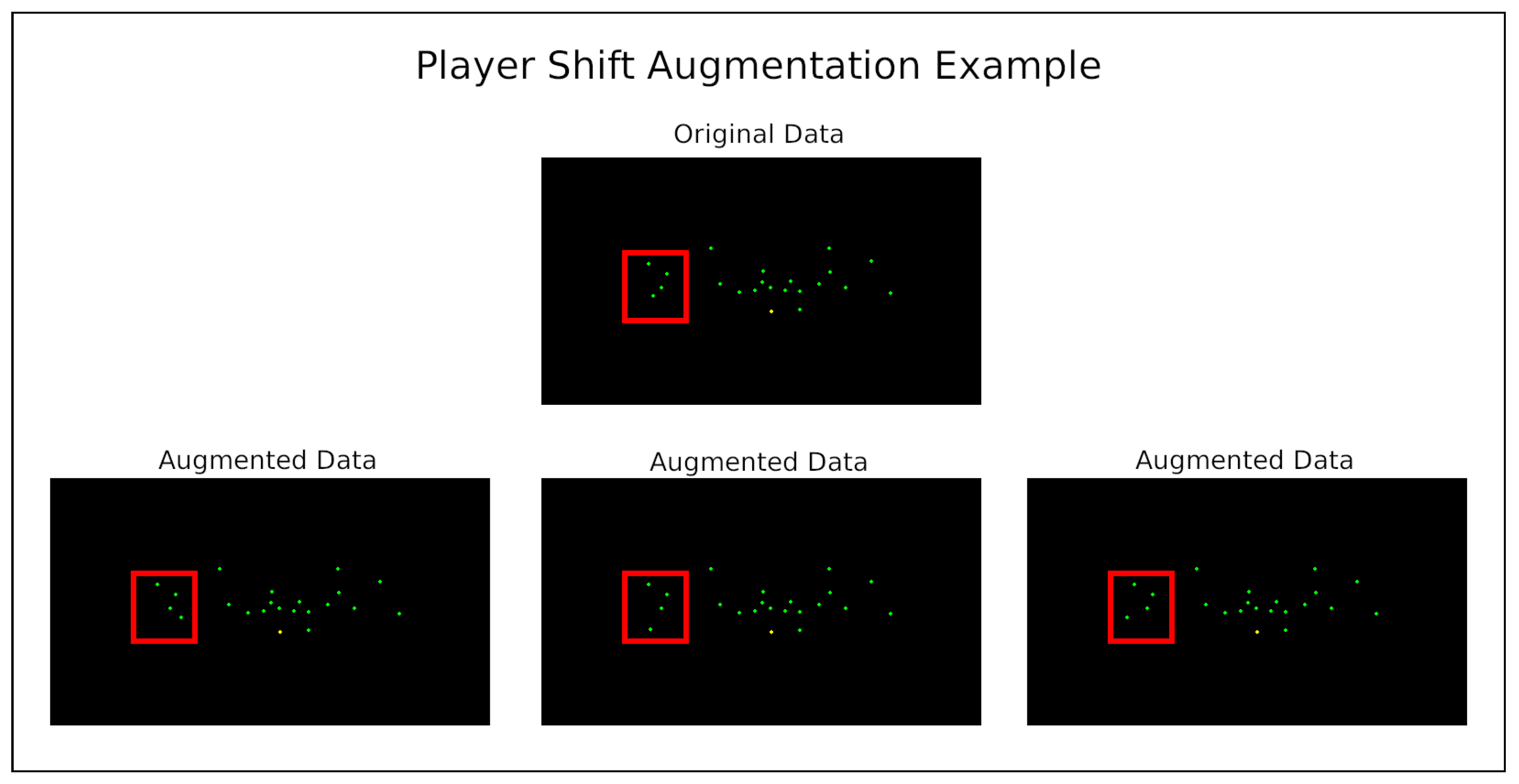
4.2.2. Player Shifting Data Augmentation
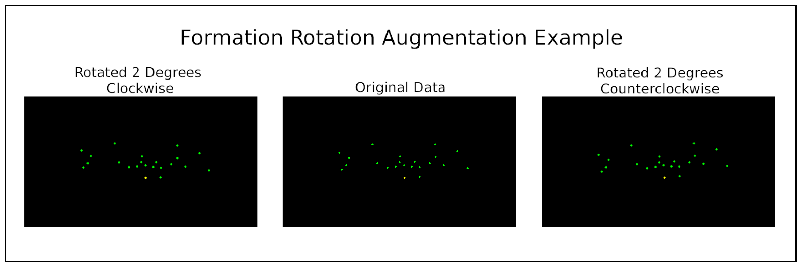
4.2.3. Formation Rotation Data Augmentation
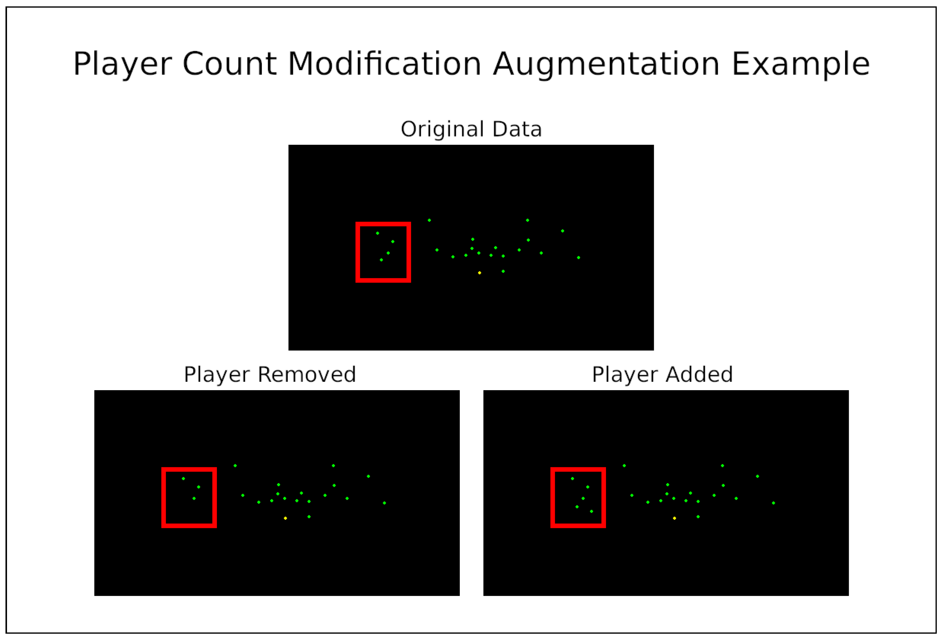
4.2.4. Player Count Modification Data Augmentation
4.3. Investigations
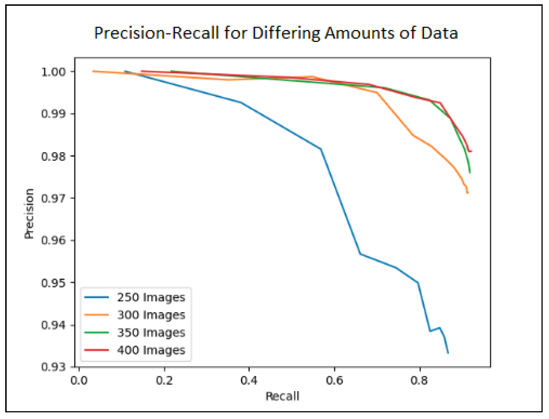
4.3.1. Dataset Size
4.3.2. Known Offense and Defense
4.3.3. Number of ResNet Layers
4.3.4. Special Rules
Quarterback Rule
Offensive Line Rule
Running Back Rule
4.3.5. Identifying the Formation without Player Labels
5. Results
5.1. Performance of Player Localization Module
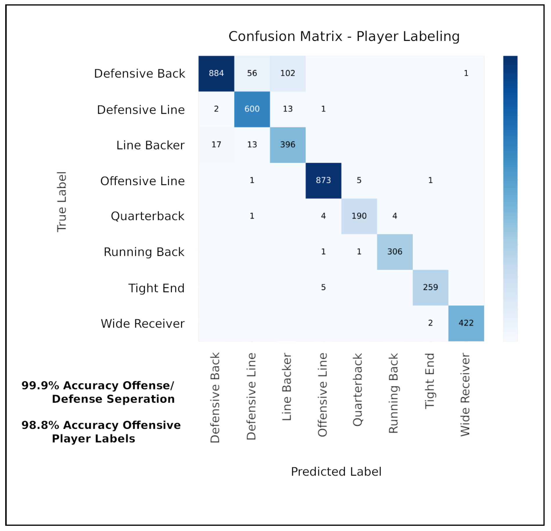
5.2. Performance of Player-Labeling Module
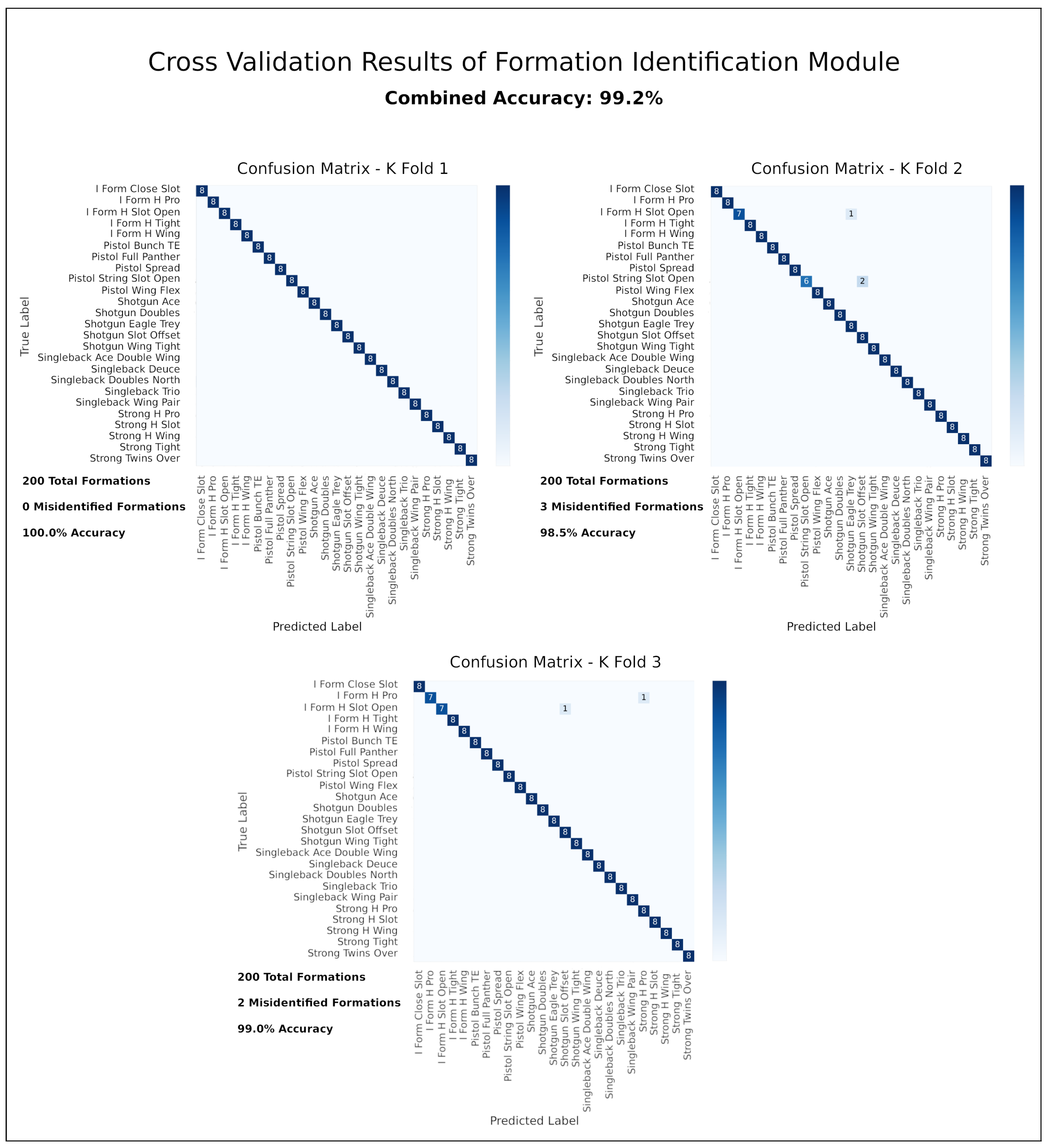
5.3. Performance of Formation Identification Module
5.4. Combining Player Localization and Player-Labeling Modules
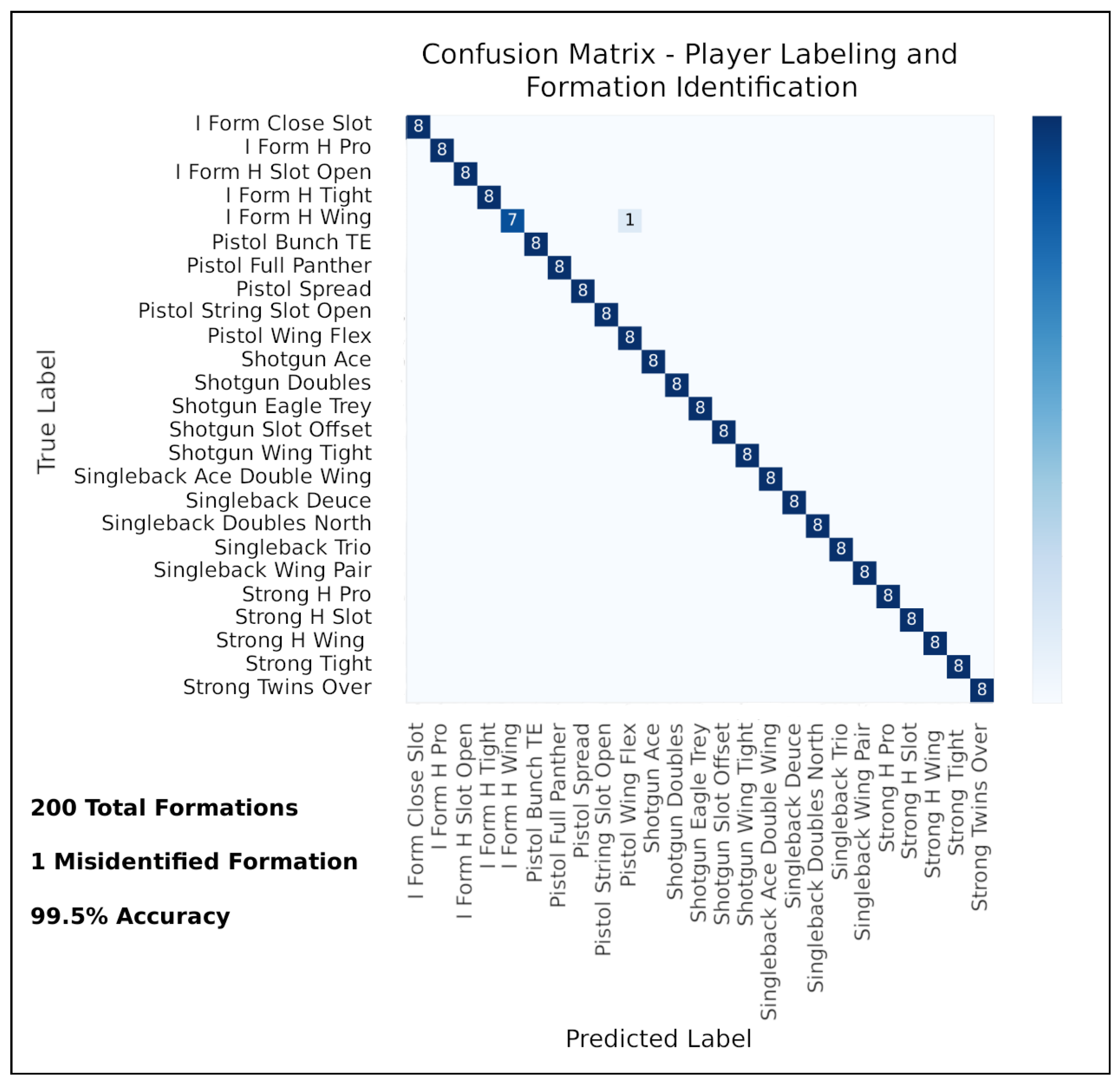
5.5. Combining Player Labeling and Formation Identification Modules
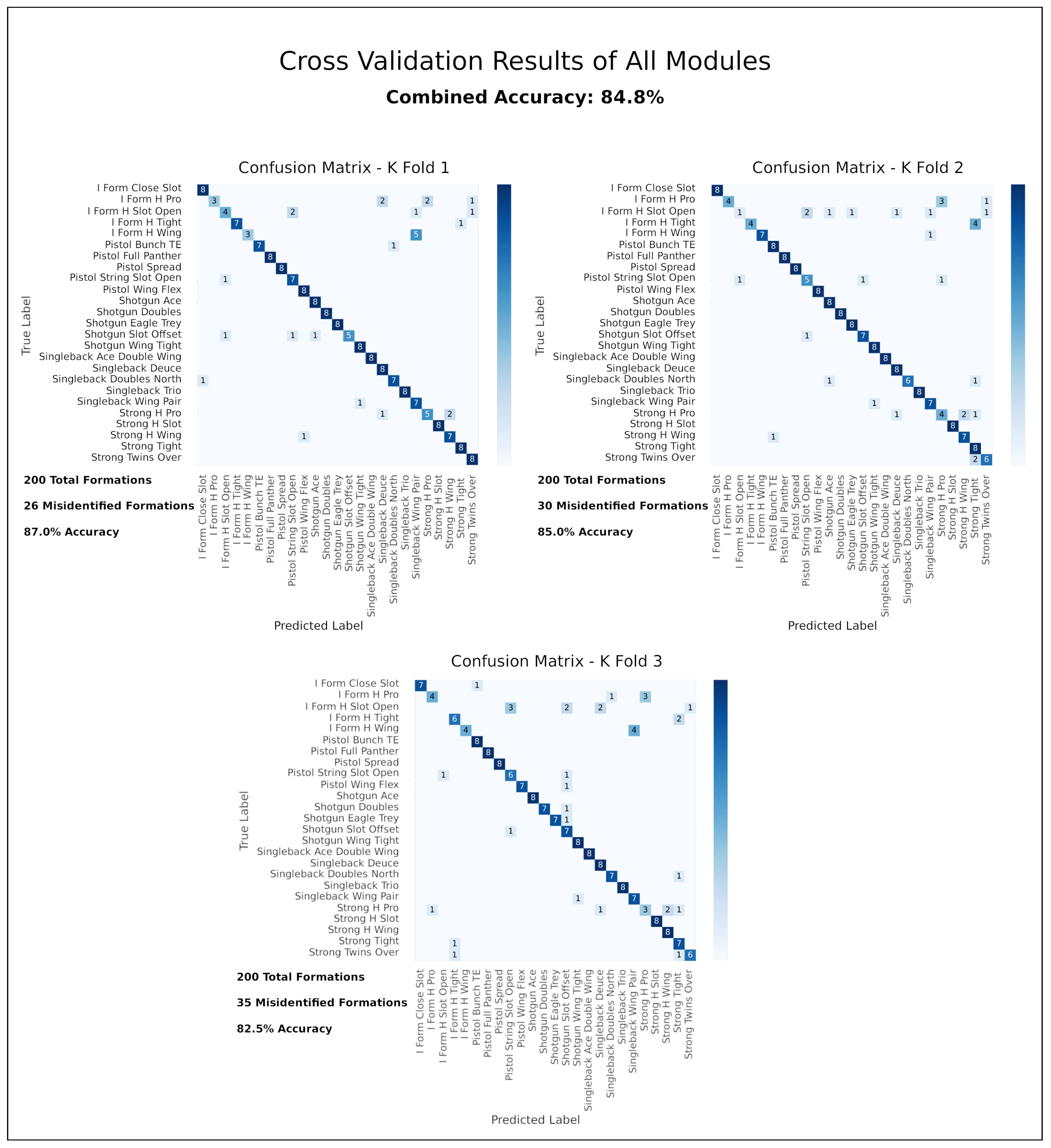
5.6. The Complete System with All Three Modules
6. Future Work
7. Conclusions
Author Contributions
Funding
Data Availability Statement
Conflicts of Interest
References
- Lu, W.; Ting, J.; Little, J.J.; Murphy, K.P. Learning to Track and Identify Players from Broadcast Sports Videos. IEEE Trans. Pattern Anal. Mach. Intell. 2013, 35, 1704–1716. [Google Scholar] [CrossRef] [PubMed]
- Koutsia, A.; Nikos, G.; Dimitropoulos, K.; Karaman, M.; Goldmann, L. Football player tracking from multiple views: Using a novel background segmentation algorithm and multiple hypothesis tracking. In Proceedings of the International Conference on Computer Vision Theory and Applications, Barcelona, Spain, 8–11 March 2007; pp. 523–526. [Google Scholar]
- Zhang, T.; Ghanem, B.; Ahuja, N. Robust multi-object tracking via cross-domain contextual information for sports video analysis. In Proceedings of the 2012 IEEE International Conference on Acoustics, Speech and Signal Processing (ICASSP), Kyoto, Japan, 25–30 March 2012; pp. 985–988. [Google Scholar] [CrossRef]
- Lee, N.; Kitani, K.M. Predicting wide receiver trajectories in American football. In Proceedings of the 2016 IEEE Winter Conference on Applications of Computer Vision (WACV), Lake Placid, NY, USA, 7–10 March 2016; pp. 1–9. [Google Scholar] [CrossRef]
- Ming, X.; Orwell, J.; Jones, G. Tracking football players with multiple cameras. In Proceedings of the 2004 International Conference on Image Processing (ICIP ’04), Singapore, 24–27 October 2004; Volume 5, pp. 2909–2912. [Google Scholar] [CrossRef]
- Atmosukarto, I.; Ghanem, B.; Saadalla, M.; Ahuja, N. Recognizing Team Formation in American Football. In Computer Vision in Sports; Moeslund, T.B., Thomas, G., Hilton, A., Eds.; Springer International Publishing: Cham, Switzerland, 2014; pp. 271–291. [Google Scholar] [CrossRef]
- Burke, B. DeepQB: Deep learning with player tracking to quantify quarterback decision-making & performance. In Proceedings of the 13 th MIT Sloan Sports Analytics Conference, Boston, MA, USA, 1–2 March 2019. [Google Scholar]
- Lhoest, A.U. Deep Learning for Ball Tracking in Football Sequences. Master’s Thesis, Université de Liège, Liège, Belgium, 2020. [Google Scholar]
- Ma, Y.; Feng, S.; Wang, Y. Fully-Convolutional Siamese Networks for Football Player Tracking. In Proceedings of the 2018 IEEE/ACIS 17th International Conference on Computer and Information Science (ICIS), Singapore, 6–8 June 2018; pp. 330–334. [Google Scholar] [CrossRef]
- Redmon, J.; Divvala, S.; Girshick, R.; Farhadi, A. You Only Look Once: Unified, Real-Time Object Detection. arXiv 2015. [Google Scholar] [CrossRef]
- Redmon, J.; Farhadi, A. YOLOv3: An Incremental Improvement. arXiv 2018. [Google Scholar] [CrossRef]
- Meuhlemann, A. TrainYourOwnYOLO: Building a Custom Object Detector from Scratch. 2019. Available online: https://github.com/AntonMu/TrainYourOwnYOLO (accessed on 30 January 2023).
- Kathuria, A. What’s New in YOLO v3? viso.ai. 23 April 2018. Available online: https://towardsdatascience.com/yolo-v3-object-detection-53fb7d3bfe6b (accessed on 30 January 2023).
- He, K.; Zhang, X.; Ren, S.; Sun, J. Deep Residual Learning for Image Recognition. arXiv 2015. [Google Scholar] [CrossRef]
- Microsoft. VOTT Visual Object Tagging Tool. 2020. Available online: https://github.com/microsoft/VoTT (accessed on 30 January 2023).


| Player Positions | Player Labels |
|---|---|
| Center | Offensive Line |
| Offensive Guard | |
| Offensive Tackle | |
| Quarterback | Quarterback |
| Running Back | Running Back |
| Tight End | Tight End |
| Wide Receiver | Wide Receiver |
| Cornerback | Defensive Back |
| Safety | |
| Defensive End | Defensive Line |
| Defensive Tackle | |
| Linebacker | Linebacker |
| Personnel | RBs | TEs | WRs |
|---|---|---|---|
| 00 | 0 | 0 | 5 |
| 10 | 1 | 0 | 4 |
| 11 | 1 | 1 | 3 |
| 12 | 1 | 2 | 2 |
| 13 | 1 | 3 | 1 |
| 14 | 1 | 4 | 0 |
| 20 | 2 | 0 | 3 |
| 21 | 2 | 1 | 2 |
| 22 | 2 | 2 | 1 |
| 23 | 2 | 3 | 0 |
| 32 | 3 | 2 | 0 |
| Formation Family | Formations |
|---|---|
| I Form | I Form Close Slot |
| I Form H Pro | |
| I Form H Slot Open | |
| I Form H Tight | |
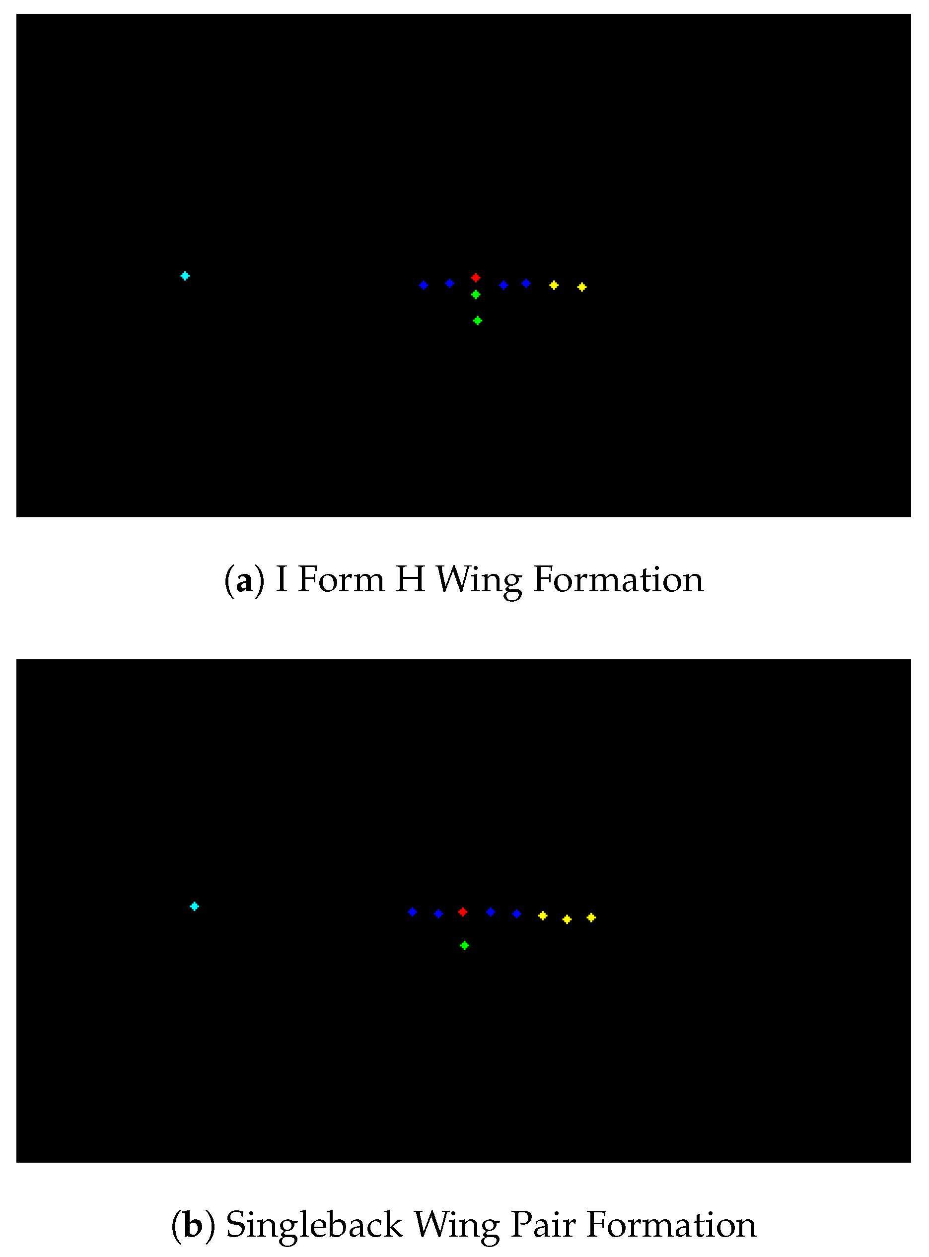
| I Form H Wing | |
| Pistol | Pistol Bunch TE |
| Pistol Full Panther | |
| Pistol Spread | |
| Pistol Strong Slot Open | |
| Pistol Wing Flex | |
| Shotgun | Shotgun Ace |
| Shotgun Doubles | |
| Shotgun Eagle Trey | |
| Shotgun Slot Offset | |
| Shotgun Wing Tight | |
| Singleback | Singleback Ace Double Wing |
| Singleback Deuce | |
| Singleback Doubles North | |
| Singleback Trio | |
| Singleback Wing Pair | |
| Strong | Strong H Pro |
| Strong H Slot | |
| Strong H Wing | |
| Strong Tight | |
| Strong Twins Over |
| Method | Input | Accuracy |
|---|---|---|
| Yolov3: Player Localization Module |  Raw Image | 90.3% |
| ResNet: Player-Labeling Module |  Player Localized Image | 98.8% |
| ResNet: Formation Identification Module |  Player Labeled Image | 99.2% |
| ResNet: Player Labeling Module and ResNet: Formation Identification Module |  Player Localized Image | 99.5% |
| Yolov3: Player Localization Module and ResNet: Player Labeling Module and ResNet: Formation Identification Module |  Raw Image | 84.8% |
Disclaimer/Publisher’s Note: The statements, opinions and data contained in all publications are solely those of the individual author(s) and contributor(s) and not of MDPI and/or the editor(s). MDPI and/or the editor(s) disclaim responsibility for any injury to people or property resulting from any ideas, methods, instructions or products referred to in the content. |
© 2023 by the authors. Licensee MDPI, Basel, Switzerland. This article is an open access article distributed under the terms and conditions of the Creative Commons Attribution (CC BY) license (https://creativecommons.org/licenses/by/4.0/).
Share and Cite
Newman, J.; Sumsion, A.; Torrie, S.; Lee, D.-J. Automated Pre-Play Analysis of American Football Formations Using Deep Learning. Electronics 2023, 12, 726. https://doi.org/10.3390/electronics12030726
Newman J, Sumsion A, Torrie S, Lee D-J. Automated Pre-Play Analysis of American Football Formations Using Deep Learning. Electronics. 2023; 12(3):726. https://doi.org/10.3390/electronics12030726
Chicago/Turabian StyleNewman, Jacob, Andrew Sumsion, Shad Torrie, and Dah-Jye Lee. 2023. "Automated Pre-Play Analysis of American Football Formations Using Deep Learning" Electronics 12, no. 3: 726. https://doi.org/10.3390/electronics12030726
APA StyleNewman, J., Sumsion, A., Torrie, S., & Lee, D.-J. (2023). Automated Pre-Play Analysis of American Football Formations Using Deep Learning. Electronics, 12(3), 726. https://doi.org/10.3390/electronics12030726