FIImap: Fast Incremental Inflate Mapping for Autonomous MAV Navigation

Abstract

Three-dimensional mapping is an essential component of autonomous Micro Aerial Vehicle (MAV) navigation. The paper focuses on the 3D spatial representation method of MAV to overcome the collision problem caused by soft constraints, control error, and planning with the center of mass by inflating the occupancy grid map. A fast incremental inflated map construction method is proposed, which reduces the time-consumption caused by the increase of map range and inflated size. The method focuses on areas of the map that occupied state changes and introduces two arrays that record newly appearing and disappearing obstacles. Then, a series of breadth-first search algorithms are used to traverse the parts of the inflated map that need local modification to update the inflated map. Moreover, a sliding map model is designed based on the MAV position, which is suitable for large-range autonomous flight. The effectiveness of the proposed approach is verified with simulated and actual flight data. The proposed method takes about 3 ms to construct the inflated map with a local update range of 16 m × 16 m × 6 m.

1. Introduction

In recent years, Micro Aerial Vehicles (MAVs) have been widely used due to their high agility and load capacity in the fields of power inspection [1,2], autonomous exploration [3,4], and emergency rescue [5,6,7,8,9]. Real-time autonomous mapping and planning in unknown and unstructured environments are critical technologies for MAVs in these applications [10,11]. A virtual occupied area nearby the obstacle is a must in many optimization-based planning algorithms [12,13]. Inflated mapping records the real and virtual occupied areas that MAVs cannot cover.

Three-dimensional mapping bridges the environment and trajectory planning [14]. Trajectory planning needs to consider safety costs, which is the function of the distance from the path to objects obtained by mapping [13,15]. Mapping models the environment and records the obstacles’ size, location, or distance fields for planners.

Currently, the main maps for planners can be categorized into topological maps [16,17] and metric maps [18]. Topological maps express the relationships among objects in graphs, such as Voronoi [17,19]. Topological maps have the advantages of small storage and search costs. However, the construct algorithm’s complexity for topological maps is high, and the real-time performance could be poor [20,21]. A metric map precisely expresses the space with regular voxels, such as a grid map [18,22]. The metric map is efficient for constructing and representing free, occupied, and unknown areas. However, it requires a large storage memory due to the huge number of nodes with a small resolution. In addition, the k-dimensional tree (KD-Tree) [23] and Euclidean Signed Distance Field (ESDF) [14] record the distance information from the nearest obstacles more effectively. Gao et al. [23] and Florence et al. [24] organized point clouds into a point cloud map via KD-Tree and obtained the distance by the nearest neighbor query algorithm.

Trajectory planning is a multi-objective optimization problem suffering from several issues. The first is that many planning algorithms use the center of mass to reduce the size of optimization variables, which abstracts the MAV as a point and ignores shapes [25,26]. The second is that distance constraints are usually expressed as soft constraints to make the trajectory optimization an unconstrained optimization problem [12,15,27]. Even if a significant safety distance threshold is chosen, the desired path can be close to the obstacles. The third is that the depth perception and control accuracy may be poor, leading to aircraft crashes. Therefore, inflated mapping is the primary method to solve these problems. Inflating the objects to a specific size decided by the size of the MAV based on the naive map is one of the crucial methods to ensure safety [12,28].

Map inflation is usually a necessary process for planners to improve safety. The inflated map expands obstacles by a specific size based on the naive map to form virtual occupied areas [27]. Due to limited onboard computational resources, many researchers [29,30] have chosen occupancy maps with large memory to improve real-time performance. Generally, occupancy maps use voxel grids to store the occupancy probability via stereo visions or LIDARs to obtain depth information. Occupancy grid maps use regular cubes to model the environment. The construction of grid maps is straightforward and very efficient. OctoMap [18] uses an octree data structure to minimize the amount of map storage while ensuring real-time performance. However, a shortcoming of the occupancy map is that the map size is a priori. Voxels Hash [31] is a method by which to make the map dynamically allocated, but it may reduce real-time performance. Most algorithms are focused on solving the problem of fast construction of occupancy grid maps without rapid inflation.

For many optimization-based motion planning algorithms, it is necessary to form virtual occupied areas. Ego-planner [12] and fast-planner [13] are batch-type inflated mapping algorithms that specify the inflated size and inflate along the triaxial direction for all objects in the update range. However, when the range of local maps increases, the time consumed by these mapping methods, especially inflated mapping, significantly increases, affecting flight efficiency and safety. Ayawli et al. [32] used the open operation in morphology to inflate obstacles and handle expansion more flexibly. The core of the expansion algorithm lies in determining the size of the safety margin. When the MAV wheelbase is larger, the margin of safety for inflating accordingly increases. At the same time, a more significant margin of safety can reduce the requirements for depth measurement accuracy and control precision. When the expansion size and local update range are small, the additional computational volume introduced by inflation can be negligible. However, the batch-style inflation algorithm is significantly more time-consuming in the face of MAVs with larger wheelbases, which require more extensive updated ranges and inflated sizes. In addition, the ego-planner requires the initial allocation of map size and cannot be adjusted in real-time, limiting the flight range.

In autonomous flight, the changes in the obstacles are local and incremental in the environment. As the map update range increases, the batch-style algorithm must repeatedly update many objects, the positions of which have not changed, reducing the real-time performance of the algorithm [21]. Many algorithms successfully apply the idea of incremental construction to build maps. Voxblox [33] identifies moving objects in the environment based on changes in TSDF values and updates the distance field of these objects. Fiesta [30] updates the grid map based on newly occupied and newly free voxels. In addition, it uses doubly linked lists to record the voxels with changing states and the indexes of the nearest obstacles. However, Fiesta is complex to implement, not only introducing a series of data structures that increases the algorithm space complexity, but also assigning a fixed map size. Voxblox and Fiesta incremental algorithms are oriented towards gradient field construction and lack use cases for inflated maps.

This paper proposes the Fast Incremental Inflate mapping (FIImap) algorithm for MAV mapping, and a sliding grid map model is designed. As computer storage is cheap, the inflated map algorithm updates the occupancy grid map based on depths and odometry. The occupancy grid map is built by the Bayes algorithm [18]. The ray casting integrates the depth measurement data into the map [34]. Then the lower and raise arrays are introduced to record the newly appeared and newly disappeared voxels, respectively. Furthermore, a batch breadth-first search (BFS) algorithm inflates voxels motivated by incremental local updates and water wave transfer [21].

The main contributions of this paper can be summarized as follows:

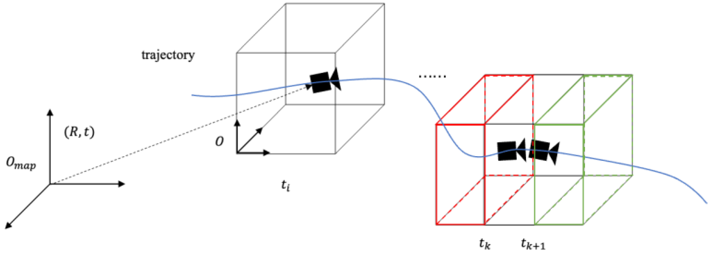
• In Euclidean space, a sliding occupancy map model is designed to support flight without map boundaries.
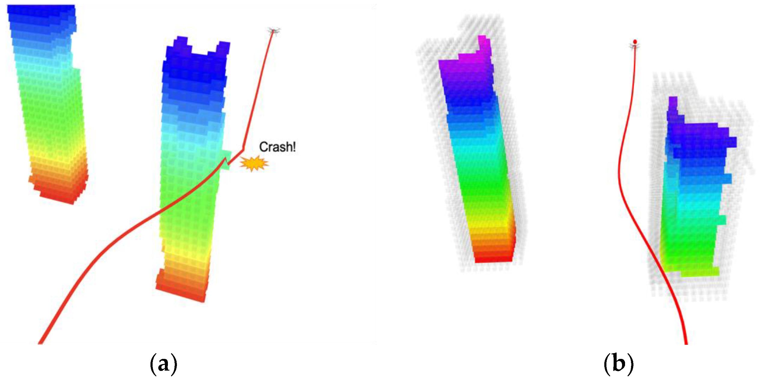
• An incremental inflated mapping algorithm based on the batch BFS algorithm is proposed, effectively improving the inflated map and updating the efficiency with a wide-range map and larger inflated size. The algorithm requires only two extra arrays for inflating operations.
• In the experiments, the effect of voxel resolution, inflated size, and the change score of the scene on the proposed algorithm’s time complexity is analyzed using different real-world data. Compared with the mapping module of ego-planner, the FIImap is more efficient under large inflated and big map sizes.

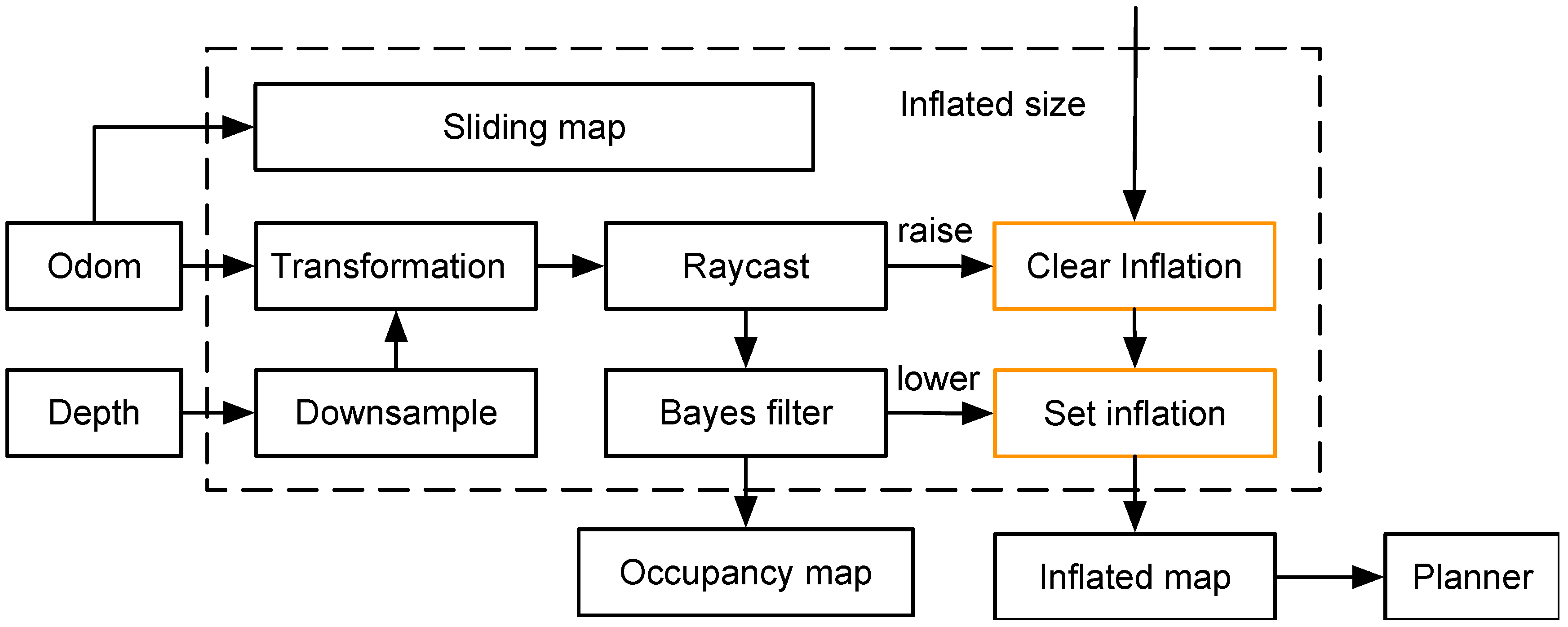
The rest of this work is organized as follows: Section 2 depicts the general framework of the algorithm. Section 3 discusses the construction method of the occupancy grid map. The proposed incremental expansion algorithm is elaborated on in Section 4. Experiments and results are analyzed in detail in Section 5. The concluding remarks are given in Section 6.

2. System

The proposed method updates the occupancy map layer and the inflated map layer, as shown in Figure 1. The system obtains odometry from the Global Navigation Satellite System (GNSS) or visual-internal odometry, and depth from stereo vision, lidar, or millimeter wave radar. Then, after time alignment, FIImap converts the down-sampled depth to a point cloud in the world frame. Then, the depth information is fused into the map via ray casting and the Bayes filter algorithm is used to update the occupancy probability. In each update stage, the voxel index from free to occupied is recorded into a lower array, and the index of the voxel from occupied to free is recorded into a raise array. Finally, the inflated value is updated using the modified BFS algorithm for the voxel in the neighbor of lower and raise, respectively. Therefore, the downstream planner can query the occupancy information in the inflated map layer. In addition, the system changes the map’s origin to slide the map based on the odometry sequence, which enables the MAV to unlimitedly and autonomously fly.

3. Occupancy Grid Map

In the Euclidean three-dimensional space, the grid map divides the workspace into a series of regular voxels, which are cubes of a size determined by the resolution. These voxels contain the occupancy probability and the inflated status [12,18]. The occupancy probability indicates whether the voxel is occupied by an obstacle, and the inflated status indicates that the voxel is occupied by a virtual obstacle. In this section, the model of the occupancy grid map, the depth map processing method, and the occupancy probability update algorithm are detailed.

3.1. Sliding Map Model

A grid map consists of a series of regular voxels uniquely determined by the size, resolution, and map origin. In this paper, a 3D grid map is designed that slides according to the position of the MAV, as shown in Figure 2. The map is stored in the form of an array. In the access of the array, it can shift the index to the beginning of the array when the index crosses the boundary at the end of the array. Therefore, the map origin is adjusted according to the translation of the odometry without creating additional storage space, and some unnecessary map data is deleted in real time.

To obtain the occupancy information of a point $p^W$, firstly calculate the voxel coordinate of $p^W$:

$$voxel=\left(p^W-p_C^W\right) mod r$$

(1)

where $p_C^W$ denotes the origin of the map in the world coordinate system, which is fixed or moves with the odometry. $r$ is the map resolution.

Then, according to the map storage method, calculate the index. The occupancy probability value of $p^W$ is accessed at the index:

$$index=size\left(0\right)\times size\left(1\right)\times voxel\left(0\right)+size\left(1\right)\times voxel\left(1\right)+voxel\left(2\right)$$

(2)

where the $index$ indicates the voxel’s position in the array, and the $size$ means the size of the map.

3.2. Processing Depth

Assume that the depth image is obtained by stereo vision, noted as $D\in R^{H\times W}$. After time aligning, the point cloud in the world frame is calculated as:

$$p^W=RK{D}_{u,v,d}+t$$

(3)

where K is the internal reference matrix of stereo vision, $D_{u,v,d}$ is a depth image, and $\left(R,t\right)$ is odometry, which denotes the coordinate transformation from the body frame to the world frame.

Downsampling is performed in the filtering procedure thanks to the depth being clean enough [24]. According to the resolution of the grid map, a suitable step can be chosen to reduce the computational effort without reducing the map’s accuracy. Taking two points, $D_1=\left(u_1,v_1,d_1\right)$ and $D_2=\left(u_2,v_2,d_2\right)$ in $D\in R^{H\times W}$, the actual coordinate difference between two points in the world frame is denoted as:

$$p_1^W-p_2^W=RK\left(D_1-D_2\right)$$

(4)

The value of the depth image is assumed to continue when the map resolution is small, which means that the depth jumps at the edges of objects are ignored. The parameter selection for sampling can be decided by the maximum measurement of the depth image, which can be denoted as:

$$\{\begin{array}{c}\Delta u=\frac{f_x}{d_{max}}r\\ \Delta v=\frac{f_y}{d_{max}}r\end{array}$$

(5)

where $\mathsf{\Delta }u$ and $\mathsf{\Delta }v$ are the vertical and horizontal downsampling step, $f_x$ and $f_y$ are focal of the depth camera, $d_{max}$ is the maximum depth value decided by experts, $r$ is the map resolution.

3.3. Updating Probability

The occupancy probability value range is in (0, 1), with larger values indicating a higher probability of the voxel being occupied. Assuming that the observation process of the map is Markovian and the voxels are measured independently of each other, the Bayes filter algorithm [18] is used to update the probability:

$$P\left(m_t\right)={\left[1+\frac{1-P\left(m|D_t,x_t\right)}{P\left(m_t|D_t,x_t\right)}\frac{1-P\left(m_{t-1}\right)}{P\left(m_{t-1}\right)}\frac{p\left(m_0\right)}{1-p\left(m_0\right)}\right]}^{-1}$$

(6)

where $D_t$ is the observed depth at $t$, $x_t$ is the pose of the MAV at $t$; $P(m_t)$ and $P(m_{t-1})$ denote the probability of the occupancy grid map at $t$ and $t-1$; $p\left(m_0\right)$ is the initial probability of the map; $P\left(m|D_t,x_t\right)$ is inverse sensor model that represents the value of the probability change of the map due to the depth measurement at $t$.

Use the log-odds occupancy value $L\left(x\right)=log\frac{P\left(x\right)}{1-P\left(x\right)}$ to rewrite Equation (6):

$$L\left(m_t\right)=L\left(m_{t-1}\right)+L\left(m|D_t,x_t\right)-L\left(m_0\right)$$

(7)

When multiple depths give measurements of the same location several times, the occupancy of the voxel gradually increases. Then, when the object here disappears, the occupancy takes at least the same period of observation length to clear. Therefore, the maximum and minimum constraints are added to Equation (7) to compensate for dynamic environments:

$$L\left(m_t\right)=min\left\{max\left[L\left(m_{t-1}\right)+L\left(m|D_t,x_t\right)-L\left(m_0\right),L_{min}\right],L_{max}\right\}$$

(8)

The prior probability of the map is set to 0.5, i.e., $L\left(m_0\right)=0$, indicating that the map knows nothing about occupancy. The inverse sensor model $L\left(m|D_t,x_t\right)$ is the logarithmic update probability after the observation of the voxel. As ray casting traverses the entire depth, the occupancy of voxels along the ray is reduced and the occupancy of voxels that are hit is increased. The $L_{min}$ and $L_{max}$ are used to balance the random error of the depth measurements with the dynamic.

4. The Proposed Incremental Inflated Mapping Algorithm

The inflated map expands the objects by a specific size to form a virtual area, which the center of MAV mass should not reach [12]. The proposed algorithm focuses on the voxels with an occupancy status that has continuously changed due to the odometry changes. These voxels are changed because of the movement of the MAV or the noise of sensor measurements. The designed lower and raise arrays are used to record the indexes of voxels, the occupancy status of which has changed from free to occupied and from occupied to free, respectively. Then, the batch BFS algorithm is used to process lower and raise. An example of the method in 2-dimensional space is given in Figure 3.

4.1. Inflating Update for the Raise Array

The proposed algorithm regards the inflated voxels as the “territory” of the voxels that are occupied. In three-dimensional Euclidean space, if the expansion set is convex, then each voxel’s “territory” is also convex. In this section, FIImap uses the raise array to record the voxels whose occupancy has changed from occupied to free. The algorithm is shown in Algorithm 1. Firstly, the raise array is initialized. When the occupancy map is updated, the voxels with the changed state are inserted into the raise array and used as the input of the algorithm. Then, the inflated state of the raise array is cleared. Then, the BFS algorithm is performed for each element in the raise array once. During the process, the neighbor’s inflated status is cleared when it is free. Otherwise, the neighbor is inserted into the temp array. The connectivity determines which neighbors are visited [30]. The boundary of the BFS algorithm is determined by the MAV size and control uncertainty, usually set as once or twice the resolution.

Algorithm 1 Inflate the map for raise array

Input: Raise (the array recording indexes of new free voxels).

Add the voxels with an occupancy state that changed from occupied to free to the raise array when updating the occupancy map; Set the inflation for all elements in the lower array; Clear the inflation for all elements in the raise array; Set the update range as $2\times L$ and specify the connectivity, and separately use the BFS algorithm for each element in the raise array. Added the voxels that are occupied to the temp array; otherwise, clear the inflated status.  Output: Inflate map.

4.2. Inflating Update for the Lower Array

The lower array is handled in a similar way to the raise array, by setting the “territory” of the voxels in the lower to be inflated. The lower array is made of two components: one is the newly occupied voxels that appear in the occupancy update, and the other is the voxels that need to be re-inflated due to incorrectly clearing while processing the raise array. Similarly, all voxels within the lower array are separately processed using the BFS algorithm, as shown in Algorithm 2. If the neighbors are not inflated, then they are set, and the neighbors’ neighbors are further traversed. When all the lower arrays have been processed, the new inflated map is updated to the latest status.

Algorithm 2 Inflate the map for lower array

Input: Lower (the array recording indexes of new occupied voxels).

Add the voxels with a state that becomes occupied to the lower array at the occupancy update stage; add all elements to the lower array that are in the temp data at updating the raise array. Set the inflation for all elements in the lower array; Set the update range as $L$ and specify the connectivity, and separately use the BFS algorithm for each element in the lower array to set the inflated status.  Output: Inflate map.

4.3. The BFS’s Escape Conditions

The BFS is the underlying algorithm for handling raise and lower. This section covers the escape conditions of the BFS that are designed to speed up inflating. When the inflated range is set to $L$, all voxels within a sphere of radius $L$ are traversed. However, during the processing of the raise, the BFS search boundary is $2L$, ensuring that all occupied voxels that need to be reassigned as “territories” are traversed. This trick saves memory by avoiding introducing a series of extra arrays to record the source of each inflated voxel [13]. Due to sensor noise and the appearance of new objects, changing voxels are often on the surface of existing objects. Therefore, the search stage can break earlier when the neighbors are occupied, which can reduce the number of voxels to be traversed.

4.4. Algorithm’s Complexity Analysis

The space complexity of the proposed incremental inflated algorithm is $O\left(4n\right)$, and $n$ is the number of voxels in the map. In addition to the raise and lower arrays, there are two arrays needed to store the occupancy map and the inflated map. The size of the lower and raise arrays has a significant positive correlation to the scene dynamic, but experiments on the cow_and_lady dataset [33] and the laboratory corridor datasets with a stereo camera show that the size is much smaller than the number of map voxels.

The time complexity of map inflating depends on the number of voxels that change in space. The map inflating creates virtual occupied areas around obstacles. When inflating the map, FIImap uses the BFS algorithm to process each voxel, the occupancy value of which has been reversed. The BFS algorithm for each voxel has the same operation that traverses a certain range of neighbors. Therefore, the time consumption of the algorithm depends on the environment dynamic; assuming that the objects in the space are far enough apart and that each object occupies only a single voxel. During a certain update, the number of voxels that become occupied in the grid map is $k_1$, and the number of voxels that become free is $k_2$. During the BFS algorithm traversal, the time complexity of the operation on neighbors is $O\left(1\right)$. The time complexity is $O\left(\left(k_1+k_2\right)\times {\left(\frac{\mathrm{L}}{\mathrm{r}}\right)}^3\right)$, and L and r are the inflated size and the map resolution. However, in the actual environment, objects usually occupy continuous voxels, and the newly occupied or newly free are often the voxels on the surface of the object. Consequently, the main time consumption reason is that the lower array would be huge after processing the raise array.

5. Experiments and Results Analysis

In this section, a series of tests are conducted for the proposed algorithm’s accuracy and computational performance. In the gazebo simulator, the practicality of the algorithm is verified by replacing mapping in the ego-planner [12]. The accuracy and time performance of the inflated mapping is tested on the Cow_and_Lady dataset and the laboratory corridor dataset. The Cow-and-Lady dataset collects data via a depth camera and Vicon system in a small room [33]. In the laboratory corridor dataset, a quadrotor is used with a realsense d455 and a realsense T265 to record depth images and odometry, respectively. All of the experiments in this section are using i7 9700K at 3.60 GHz, and only one thread is used.

5.1. Simulation in the Unexplored Environment

The inflated map provides occupancy information for the planner to perform collision detection. An unstructured scene containing a shelf and several geometric objects is built by the gazebo simulator. A drone equipped with a depth camera and an odometer is used for mapping online, and the results are shown in Figure 4. The colored voxels are the occupied grids and the dark white grids are the virtual occupied grids generated from the inflated map. The map resolution is 0.05 m. During mapping, the speed of the MAV is kept at a constant value as much as possible to improve the accuracy of the odometry.

Inflated maps are the fundamental safety protection mechanism in an optimization-based planner. The maps in the ego-planner planner are replaced with FIImap to test the correctness. In optimization-based planners, most algorithms use regularization to add the distance constraints to the objective; the generated trajectories may be close to the obstacle when the smoothing coefficients are large. As shown in Figure 5a, without setting the inflation, the planner generates a trajectory that is relatively close to the obstacle. At this point, the depth measurement noise appears and the planner judges that the MAV appears to be in a collision. In Figure 5b, the inflated size is twice the resolution, and the result shows that the map inflating can move the trajectory far away from the obstacle. The map resolution of both is set at 0.2 m.

5.2. Experiments on Real-World Datasets

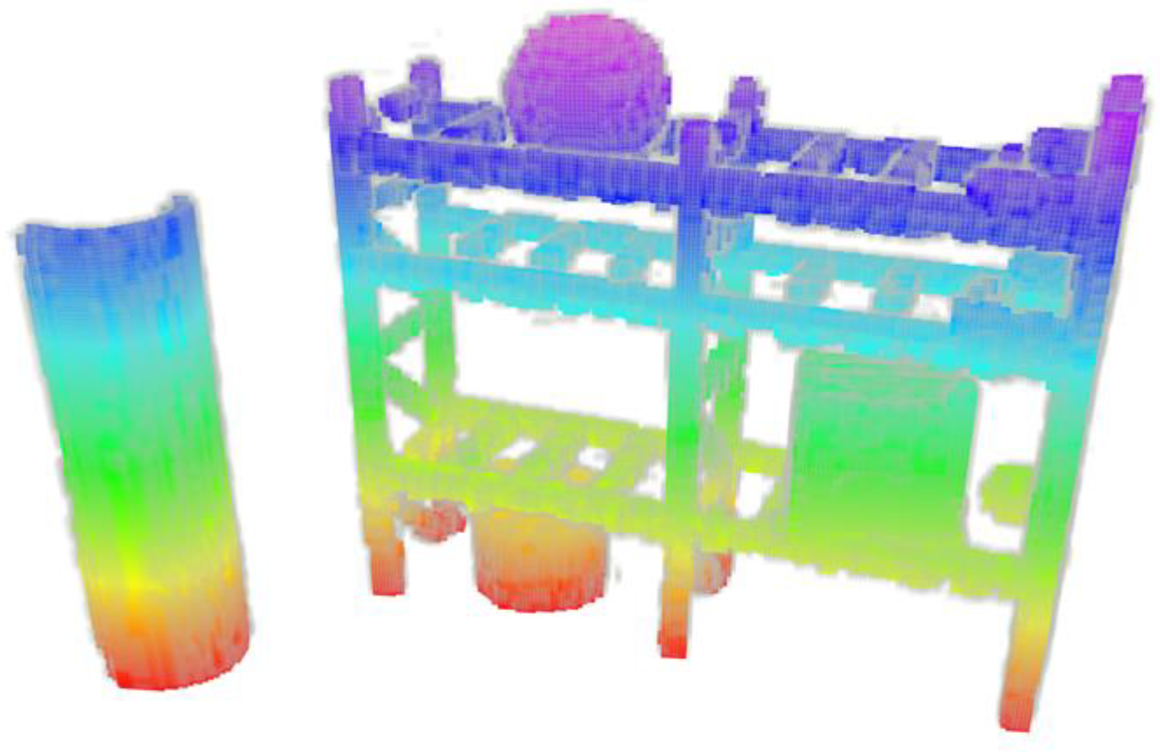
5.2.1. Accuracy Performance

An accurate model of the obstacles’ location and size is essential to flight safety. The inflated map is generated from the occupancy grid map without pruning, so the occupancy grid map’s accuracy directly suggests the inflated map’s accuracy. This paper calculates the accuracy using the cross-validation method [18]. The accuracy of the occupancy map refers to the proportion of objects measured that fall in the occupied voxels. In the cross-validation, 90% of all scans are used to build the map, and the remaining 10% are for evaluation. The results are given in

Table 1. Accuracy experiments on the laboratory corridor dataset.

Method	Resolution = 0.1 m	Resolution = 0.2 m
FIImap	91.76 $\pm$ 6.01	97.03 $\pm$ 2.76
ego-planner	92.55 $\pm$ 5.01	96.05 $\pm$ 3.76

.

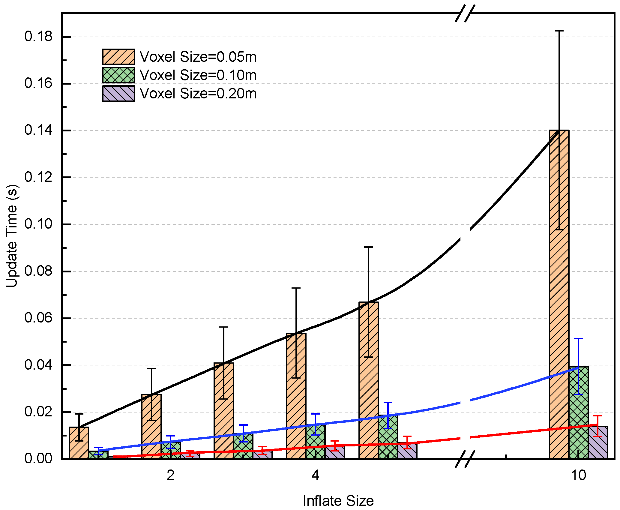
5.2.2. Time Performance with Different Parameters

In this section, the time performance is tested with different map resolutions and inflated sizes on the laboratory corridor dataset. The map resolution is usually determined by the size of MAVs and is set at 0.05 m, 0.1 m, and 0.2 m in the tests. To evaluate the effectiveness of the algorithm, the inflated size is set to 1 to 10 times the map resolution, which is recommended to be once or twice in practice. When the inflated size is too large, one can appropriately increase the map resolution. In the mapping, the sliding map size is set as 100 m $\times$ 100 m $\times$ 6 m, the local update range as 16 m $\times$ 16 m $\times$ 6 m, and the number of neighbors to 6. The update time for inflating is shown in Figure 6. According to the experimental results, the proposed algorithm is efficient at smaller inflated sizes and large resolutions. The update time sharply increases as the resolution decreases. However, the update time slowly increases at smaller inflated sizes due to the small size of lower and higher.

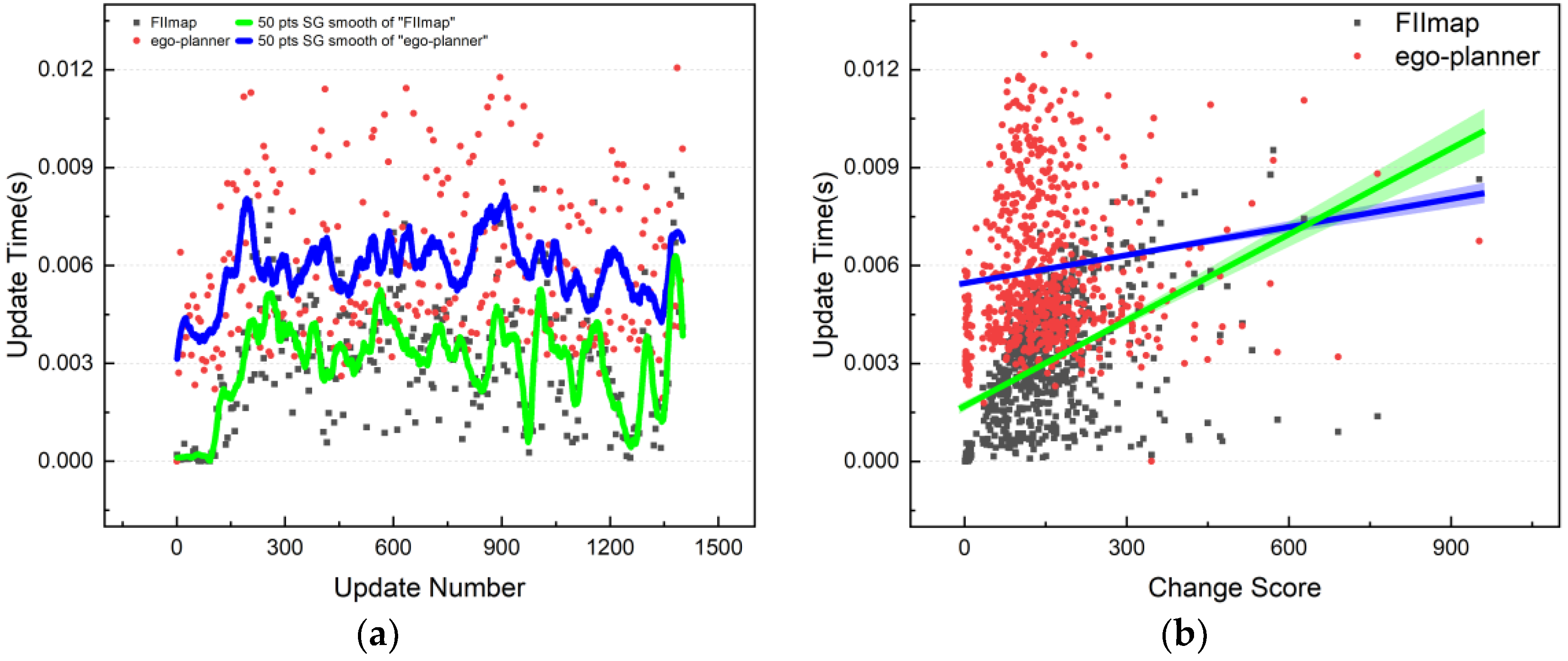
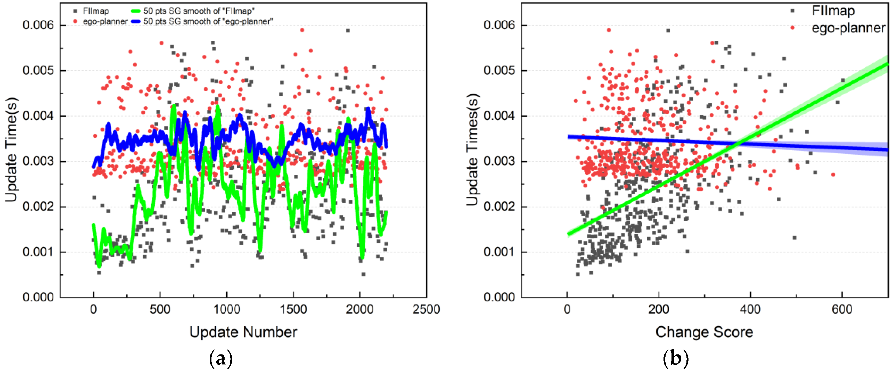
5.2.3. Comparison with Ego-Planner’s Mapping

The paper conducted a comparison experiment with the mapping module in the ego-planner framework. The Cow_and_Lady dataset and the laboratory corridor dataset were used. The ray casting distance and the maximum depth were set as 8 m in both experiments. The local update map size was 16 m $\times$ 16 m $\times$ 6 m. The results are shown in Figure 7 and Figure 8.

FIImap has a better performance on average time than the ego-planner. However, it is slightly more time-consuming than the ego-planner due to the high dynamics. Therefore, the scene change score is defined to measure the scene dynamics, which is the sum of the raise array and the lower array. To describe those worse cases more clearly, Figure 7b and Figure 8b compare the time consumption using the change score as the independent variable. Experiments show that the proposed algorithm is positively correlated with a change score that is mostly below 300. When the change score is less than 150, the single time consumption is less than the ego-planner mapping module.

6. Conclusions

Aimed toward autonomous MAV navigation in unknown environments, this paper proposed an incremental, constructing inflated map method based on sliding 3D occupancy grid maps, a depth map down-sampling method. For the method in this paper, accuracy experiments and time-consuming comparison experiments of the incremental inflation algorithm were conducted on the Cow_and_Lady dataset and the laboratory corridor dataset, respectively. The experiments showed that the accuracy of the occupancy map was higher than 90%, which is comparable to the accuracy of a typical ego-planner mapping module and could meet the demand for autonomous navigation and obstacle avoidance. The time-consuming experiments were carried out on two typical scene datasets, setting a map update range of 16 m $\times$ 16 m $\times$ 6 m. The results showed that the inflated time consumed more with higher resolution and larger inflated size. In addition, the proposed algorithm took about 3 ms on average when the inflated size was once or twice the voxel resolution when the scene change score was mild, which was better than the batch-style mapping module.

References

1. Chen, D.Q.; Guo, X.H.; Huang, P.; Li, F.H. Safety Distance Analysis of 500kV Transmission Line Tower UAV Patrol Inspection. IEEE Lett. Electromagn. Compat. Pract. Appl. 2020, 2, 124–128. [Google Scholar] [CrossRef]
2. Kim, S.; Kim, D.; Jeong, S.; Ham, J.W.; Lee, J.K.; Oh, K.Y. Fault Diagnosis of Power Transmission Lines Using a UAV-Mounted Smart Inspection System. IEEE Access 2020, 8, 149999–150009. [Google Scholar] [CrossRef]
3. Zhong, P.; Chen, B.; Lu, S.; Meng, X.; Liang, Y. Information-Driven Fast Marching Autonomous Exploration with Aerial Robots. IEEE Robot. Autom. Lett. 2022, 7, 810–817. [Google Scholar] [CrossRef]
4. Maciel-Pearson, B.G.; Akçay, S.; Atapour-Abarghouei, A.; Holder, C.; Breckon, T.P. Multi-Task Regression-Based Learning for Autonomous Unmanned Aerial Vehicle Flight Control within Unstructured Outdoor Environments. IEEE Robot. Autom. Lett. 2019, 4, 4116–4123. [Google Scholar] [CrossRef] [Green Version]
5. Chatziparaschis, D.; Lagoudakis, M.G.; Partsinevelos, P. Aerial and Ground Robot Collaboration for Autonomous Mapping in Search and Rescue Missions. Drones 2020, 4, 79. [Google Scholar] [CrossRef]
6. Liu, X.; Ansari, N. Resource Allocation in UAV-Assisted M2M Communications for Disaster Rescue. IEEE Wirel. Commun. Lett. 2019, 8, 580–583. [Google Scholar] [CrossRef]
7. Xu, X.; Qian, Y. Location-Based Hybrid Precoding Schemes and QoS-Aware Power Allocation for Radar-Aided UAV–UGV Cooperative Systems. IEEE Access 2022, 10, 50947–50958. [Google Scholar] [CrossRef]
8. Calamoneri, T.; Corò, F.; Mancini, S. A Realistic Model to Support Rescue Operations After an Earthquake via UAVs. IEEE Access 2022, 10, 6109–6125. [Google Scholar] [CrossRef]
9. Qin, H.; Meng, Z.; Meng, W.; Chen, X.; Sun, H.; Lin, F.; Ang, M.H. Autonomous Exploration and Mapping System Using Heterogeneous UAVs and UGVs in GPS-Denied Environments. IEEE Trans. Veh. Technol. 2019, 68, 1339–1350. [Google Scholar] [CrossRef]
10. Florence, P.R. Integrated Perception and Control at High Speed. Ph.D. Thesis, Massachusetts Institute of Technology, Cambridge, MA, USA, 2016. [Google Scholar]
11. Zhou, X.; Wen, X.Y.; Wang, Z.P.; Gao, Y.M.; Li, H.J.; Wang, Q.H.; Yang, T.K.; Lu, H.J.; Cao, Y.J.; Xu, C.; et al. Swarm of micro flying robots in the wild. Sci. Robot. 2022, 7, eabm5954. [Google Scholar] [CrossRef]
12. Zhou, X.; Wang, Z.P.; Ye, H.K.; Xu, C.; Gao, F. EGO-Planner: An ESDF-Free Gradient-Based Local Planner for Quadrotors. IEEE Robot. Autom. Lett. 2021, 6, 478–485. [Google Scholar] [CrossRef]
13. Zhou, B.Y.; Gao, F.; Wang, L.Q.; Liu, C.H.; Shen, S.J. Robust and Efficient Quadrotor Trajectory Generation for Fast Autonomous Flight. IEEE Robot. Autom. Lett. 2019, 4, 3529–3536. [Google Scholar] [CrossRef] [Green Version]
14. Chen, Y.Z.; Lai, S.P.; Cui, J.Q.; Wang, B.; Chen, B.M. GPU-Accelerated Incremental Euclidean Distance Transform for Online Motion Planning of Mobile Robots. IEEE Robot. Autom. Lett. 2022, 7, 6894–6901. [Google Scholar] [CrossRef]
15. Zucker, M.; Ratliff, N.; Dragan, A.D.; Pivtoraiko, M.; Klingensmith, M.; Dellin, C.M.; Bagnell, J.A.; Srinivasa, S.S. CHOMP: Covariant Hamiltonian optimization for motion planning. Int. J. Robot. Res. 2013, 32, 1164–1193. [Google Scholar] [CrossRef] [Green Version]
16. Blochliger, F.; Fehr, M.; Dymczyk, M.; Schneider, T.; Siegwart, R. Topomap: Topological Mapping and Navigation Based on Visual SLAM Maps. In Proceedings of the 2018 IEEE International Conference on Robotics and Automation (ICRA), Brisbane, Australia, 21–25 May 2018; IEEE: Brisbane, Australia, 2018; pp. 3818–3825. [Google Scholar]
17. Wallgrün, J.O. (Ed.) Voronoi-Based Spatial Representations. In Hierarchical Voronoi Graphs: Spatial Representation and Reasoning for Mobile Robots; Springer: Berlin/Heidelberg, Germany, 2010; pp. 45–58. ISBN 978-3-642-10345-2. [Google Scholar]
18. Hornung, A.; Wurm, K.M.; Bennewitz, M.; Stachniss, C.; Burgard, W. OctoMap: An efficient probabilistic 3D mapping framework based on octrees. Auton. Robots 2013, 34, 189–206. [Google Scholar] [CrossRef] [Green Version]
19. Deits, R.; Tedrake, R. Computing Large Convex Regions of Obstacle-Free Space through Semidefinite Programming. In Algorithmic Foundations of Robotics XI; Akin, H.L., Amato, N.M., Isler, V., van der Stappen, A.F., Eds.; Springer Tracts in Advanced Robotics; Springer International Publishing: Cham, Switzerland, 2015; Volume 107, pp. 109–124. ISBN 978-3-319-16594-3. [Google Scholar]
20. Kalra, N.; Ferguson, D.; Stentz, A. Incremental Reconstruction of Generalized Voronoi Diagrams on Grids. In Proceedings of the Intelligent Autonomous Systems 9(IAS-9), Tokyo, Japan, 7–9 March 2006. [Google Scholar]
21. Lau, B.; Sprunk, C.; Burgard, W. Improved updating of Euclidean distance maps and Voronoi diagrams. In Proceedings of the 2010 IEEE/RSJ International Conference on Intelligent Robots and Systems (IROS 2010), Taipei, Taiwan, 18–22 October 2010; IEEE: Taipei, Taiwan, 2010; pp. 281–286. [Google Scholar]
22. Graichen, T.; Schmidt, R.; Richter, J.; Heinkel, U. Occupancy Grid Map Generation from OSM Indoor Data for Indoor Positioning Applications. In Proceedings of the 6th International Conference on Geographical Information Systems Theory, Applications and Management, Prague, Czech Republic, 7–9 May 2020; pp. 168–174. [Google Scholar]
23. Gao, F.; Wu, W.; Gao, W.L.; Shen, S.J. Flying on point clouds: Online trajectory generation and autonomous navigation for quadrotors in cluttered environments. J. Field Robot. 2019, 36, 710–733. [Google Scholar] [CrossRef]
24. Florence, P.R.; Carter, J.; Ware, J.; Tedrake, R. NanoMap: Fast, Uncertainty-Aware Proximity Queries with Lazy Search Over Local 3D Data. In Proceedings of the 2018 IEEE International Conference on Robotics and Automation (ICRA), Brisbane, Australia, 21–25 May 2018; pp. 7631–7638. [Google Scholar]
25. Ren, Y.; Zhu, F.; Liu, W.; Wang, Z.; Lin, Y.; Gao, F.; Zhang, F. Bubble Planner: Planning High-speed Smooth Quadrotor Trajectories using Receding Corridors. arXiv 2022, arXiv:2202.12177. [Google Scholar]
26. Daftry, S.; Zeng, S.; Khan, A.; Dey, D.; Melik-Barkhudarov, N.; Bagnell, J.A.; Hebert, M. Robust Monocular Flight in Cluttered Outdoor Environments. arXiv 2016, arXiv:1604.04779. [Google Scholar]
27. Tordesillas, J.; Lopez, B.T.; How, J.P. FASTER: Fast and Safe Trajectory Planner for Flights in Unknown Environments. In Proceedings of the 2019 IEEE/RSJ International Conference on Intelligent Robots and Systems (IROS), Macau, China, 3–8 November 2019. [Google Scholar]
28. Chen, J.; Liu, T.B.; Shen, S.J. Online generation of collision-free trajectories for quadrotor flight in unknown cluttered environments. In Proceedings of the 2016 IEEE International Conference on Robotics and Automation (ICRA), Stockholm, Sweden, 16–21 May 2016; pp. 1476–1483. [Google Scholar]
29. Zhou, X.; Zhu, J.; Zhou, H.; Xu, C.; Gao, F. EGO-Swarm: A Fully Autonomous and Decentralized Quadrotor Swarm System in Cluttered Environments. In Proceedings of the 2021 IEEE International Conference on Robotics and Automation (ICRA), Xi’an, China, 30 May–5 June 2021. [Google Scholar]
30. Han, L.X.; Gao, F.; Zhou, B.Y.; Shen, S.J. FIESTA: Fast Incremental Euclidean Distance Fields for Online Motion Planning of Aerial Robots. In Proceedings of the 2019 IEEE/RSJ International Conference on Intelligent Robots and Systems (IROS), Macau, China, 3–8 November 2019. [Google Scholar]
31. Nießner, M.; Zollhöfer, M.; Izadi, S.; Stamminger, M. Real-time 3D Reconstruction at Scale using Voxel Hashing. ACM Trans. Graph. TOG 2013, 32, 1–11. [Google Scholar] [CrossRef] [Green Version]
32. Ayawli, B.B.K.; Appiah, A.Y.; Nti, I.K.; Kyeremeh, F.; Ayawli, E.I. Path planning for mobile robots using Morphological Dilation Voronoi Diagram Roadmap algorithm. Sci. Afr. 2021, 12, e00745. [Google Scholar] [CrossRef]
33. Oleynikova, H.; Taylor, Z.; Fehr, M.; Nieto, J.; Siegwart, R. Voxblox: Incremental 3D Euclidean Signed Distance Fields for On-Board MAV Planning. In Proceedings of the 2017 IEEE/RSJ International Conference on Intelligent Robots and Systems (IROS), Vancouver, BC, Canada, 24–28 September 2017; pp. 1366–1373. [Google Scholar]
34. Amanatides, J.; Woo, A. A Fast Voxel Traversal Algorithm for Ray Tracing. Eurographics 1987, 87, 3–10. [Google Scholar]
Figure 1. Schematic diagram of FIImap system.
Electronics 12 00534 g001
Figure 2. Sliding grid map model. The model is made of regular voxels, with the map origin in the lower right corner and the MAV in the center of the map, as shown at t i . The map origin is adjusted with MAV movement, and the unnecessary part (red area) is cleared. Thanks to the mapping relationship of the array index, the newly observed area (green area) is set, as shown from t k to t k + 1 .
Electronics 12 00534 g002
Figure 3. Inflated mapping update between two configurations (a,c). (a,c) show the expansion maps of the 2D raster map at moments t k 1 and t k . (b) shows the process of handling the raise array. Assume that, at t k 1 , there are three occupied grids (yellow) in the map. Assume that, at t k 1 , there are three occupied grids (yellow) in the map. At t k , a newly occupied grid (green) and a disappeared occupied grid (above blue grid) are observed. Firstly, remove the virtual occupied grid created by the raise array and add the mistakenly removed grid (blue) to the lower array. Then, the virtual occupied grid is set near the grids in the lower array to generate the whole inflate map at t k .
Electronics 12 00534 g003
Figure 4. FIIMap representation of in-progress exploration in a gazebo simulator (https://gazebosim.org/home). (accessed on 18 January 2022). The colored voxels are occupied. The dark white voxels are inflated spaces that are virtually occupied.
Electronics 12 00534 g004
Figure 5. Snapshots and inflated maps when a MAV flies through obstacles in the gazebo. (a) trajectory planning on the occupancy grid map. (b) trajectory planning on the inflated map.
Electronics 12 00534 g005
Figure 6. The performance on the laboratory corridor dataset. The sliding map size is set to 100 m × 100 m × 6 m, the connectivity is 6, the ray casting distance and maximum depth is 8 m, and the local update range is 16 m × 16 m × 6 m.
Electronics 12 00534 g006
Figure 7. Comparison on the Cow_and_Lady dataset. The resolution is 0.2 m and the inflated size is single voxel resolution. The update number axis means the time axis. (a) The time consumption with update number. (b) The time consumption with change score.
Electronics 12 00534 g007
Figure 8. Comparison of the laboratory corridor dataset. The resolution is 0.2 m and the inflated size is double voxel resolution. The update number axis means the time axis. (a) The time consumption with update number. (b) The time consumption with change score.
Electronics 12 00534 g008