Flexible Networked Machine Integrated Scheduling Algorithm Based on the Dynamic Root Node Operation Set Considering Reverse Scheduling

Abstract

Aiming at the problem that the previous flexible machine network integrated scheduling algorithm only considers positive sequence scheduling, which leads to the extension of product completion time, a reverse-order machine network integrated scheduling algorithm based on the dynamic root node operation set is proposed. In order to avoid the constraints of multi-predecessor operations in the process of forward-order scheduling, an encoding method based on dynamic root node operation set is proposed to ensure the validity of constraints among operations. The crossover methods based on crossover row vector and subtree are proposed to ensure the legitimacy of offspring individuals. The chaotic mutation method based on sibling operation and the random mutation method based on mutation row vector are proposed, respectively, to ensure the diversity of the population. A local search strategy based on the critical operation machine set is proposed, which enhances the search ability of the algorithm for optimal solutions. The comparative experimental results show that the proposed algorithm’s solving speed and solution quality outperform other comparison algorithms.

1. Introduction

In the traditional manufacturing process, processing [1,2] and assembly [3,4] are regarded as two independent stages. The current research on the problem mainly focuses on the processing stage, such as the flow shop scheduling environment [5,6] and the job-shop scheduling environment [7,8]. With the increase in the diversified demands of society, the orders of multiple varieties and small batches are gradually increasing. Driven by this diversified demand environment, a new production scheduling mode is needed to meet the needs of the people’s personalized customized products. In this way, integrated scheduling [9] emerges as the times require, which unifies the machining process and assembly process of a product into a processing process, and maps complex products into a virtual processing operation tree. Since the linear processing constraints and assembly constraints among operations are considered at the same time, the integrated scheduling problem has important research significance and practical application value in shortening the product manufacturing cycle and improving the efficiency of the production system.

At present, researchers focus more on the integrated scheduling problem in the direction of simple products [10,11], but relatively less research on the complex product integrated scheduling problem with multi-layer tree structure. The comprehensive scheduling algorithm used in the research process is mainly divided into two categories: Heuristic rule algorithm and intelligent optimization algorithm. In the first type of comprehensive scheduling algorithm based on heuristic rules, there are different dispatching rules. In this type of algorithm, a series of algorithms based on the product process tree are proposed, and the problems involved include general product integrated scheduling [12,13], integrated scheduling with special process constraints [14,15], and special single workshop comprehensive scheduling problem of equipment [16,17], and comprehensive scheduling problem of distributed multi-workshop production environment [18,19,20], etc. However, the above algorithms have certain defects. The first type of algorithm uses rule-based scheduling algorithms, which are more dependent on the processing structure of the product process, and it is difficult to adapt to the differences between different examples. Moreover, the scheduling scheme does not have diversity, and the quality of the solution cannot meet the needs very well. In the second type of algorithm, the solution to the comprehensive scheduling problem must first meet the complex priority constraints, so that the existing coding methods and evolutionary operators cannot achieve the expected results, and thus make this type of algorithm in the actual problem-solving process. restricted to a certain extent. While Wang et al. [21] and Wang et al. [22] proposed different solutions based on genetic algorithms, both of these two schemes cannot avoid the detection and repair of infeasible chromosomes generated by coding and genetic operators, making the calculation of the algorithm larger volume and lower operating efficiency. Zhao, Han and Wang [23] proposed to realize the comprehensive scheduling of products by virtualizing the level of parts and coding according to the level of partition. The algorithm first sets different grades for the components of each part of the product, and then partitions them according to different grades, and then encodes the components according to different partitions. While this coding method can improve the initial solution to a certain extent, it is feasible, but this encoding method increases the constraints of the realization process of some processes, resulting in a reduction in the space of feasible solutions and an increase in the possibility of leaving the optimal solution. Shi and Zhao [24] proposed a genetic algorithm solution based on constraint chain coding. The coding method designed ensures the feasibility and completeness of the initial solution space, but the crossover and mutation operations designed by it will produce an impossible solution, requiring additional detection and repair work. Lei, Guo and Song [25] proposed a comprehensive scheduling algorithm based on the process relationship matrix table. The algorithm first establishes a process relationship matrix table for the product, and then designs the corresponding coding rules and evolution operators based on the table. Shi, Zhao and Meng [26] proposed an algorithm that mixed the improved bottleneck equipment switching strategy and genetic algorithm, but it needs to perform different operations on different infeasible chromosomes to achieve the repair effect.

The flexible machine network integrated scheduling problem extends the traditional flexible integrated scheduling problem [27,28], that is, all kinds of machines providing processing services are no longer limited to the same physical location. Therefore, it is necessary to pay attention to the physical location of the process in practical applications and the transportation process between equipment resources. However, most of the equipment resources in the comprehensive scheduling problems studied by previous studies are geographically located in the same workshop or enterprise, and the designed algorithm ignores the process transportation between the equipment or includes the transportation time in the processing time. Such an assumption is not in line with the actual cloud manufacturing production environment and affects the final scheduling results. Therefore, in order to solve the problems faced by flexible equipment in network production scenarios, we propose a comprehensive scheduling solution for reverse-sequence equipment networks based on root node process sets that can meet real-time changes. Aiming at the priority processing constraints existing in complex products, combined with the reverse order scheduling method, a coding method that supports real-time changes based on the root node process set is given. In order to ensure that the population individuals conform to the corresponding rules during the evolution process, two available crossover and mutation operators are given, respectively.

2. Problem Description

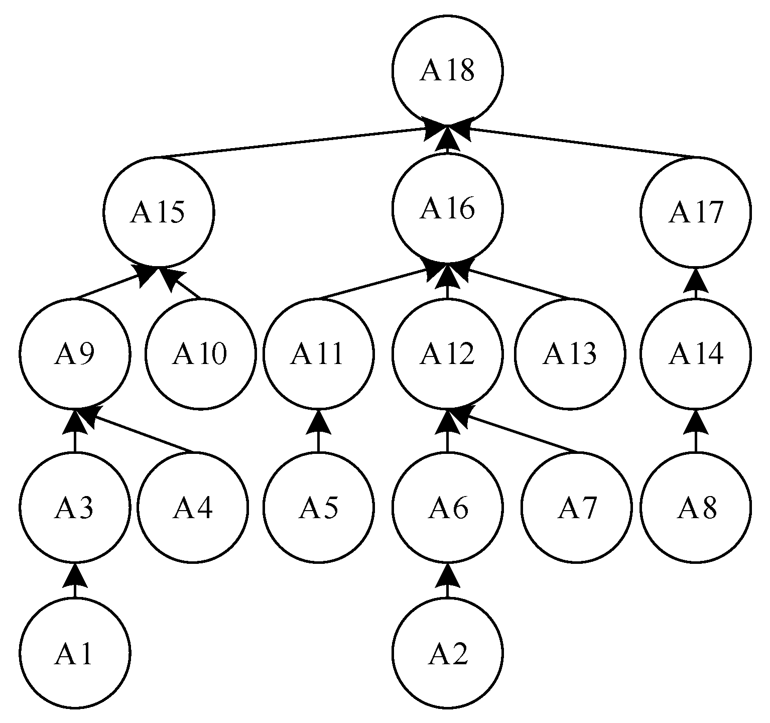
In general, the comprehensive scheduling problem of tree-structured complex products in the flexible equipment network production scenario can be understood as: A tree-structured complex product that contains n processes that can be completed and requires multiple interconnected processing equipment for collaborative production. For example, Figure 1 shows the process of a product being processed into a finished product through multiple processes. Each process includes three different parts, which are the name of the process, the set of equipment to be used in the processing process, and the process required for the process. The transportation time between the devices in Figure 1 is shown in

Table 1. The transportation time required for movement of the operation between different machines.

	M1	M2	M3	M4
M1	0	10	15	10
M2	10	0	25	20
M3	15	25	0	10
M4	10	20	10	0

. The work of this paper is to reasonably arrange the scheduling sequence of each process and the corresponding processing equipment to reduce the time spent on product processing. Assuming that the selectable process set is ${\left\{O_i\right\}}_{1\le i\le n}$, the selectable equipment set of process $O_i$ is ${\left\{M_i\right\}}_{1\le i\le n}\subseteq \left\{1,2,\dots ,m\right\}$ and $M_i\ne \varphi$, $p_{ik}$ is the time it takes for process $O_i$ to process products through equipment $m_k\in M_i. T_{M_k,M_l}$ is the transportation time between equipment $M_k$ and $M_l$. The processing sequence between processes is executed according to the order specified by the constraint relationship set $C=\left\{\left(O_i,O_j\right)|O_i,O_j\in \left\{1,2,\dots ,n\right\}\right\},$ it means that only Process $O_i$ processing operation is completed, $O_j$ can perform processing operation. $s_i$ and $c_i$ represent the processing start time and end time of $O_{i }$, respectively. $x_{ik}$ = 1 means that the process $O_i$ is processed on the equipment $m_k\in M_i$, otherwise it is 0; $y_{ij}$ = 1 means that the processes $O_i$ and $O_j$ are processed on the same equipment, and the process $O_i$ is the immediate preceding process of the process $O_j$, that is, the process $O_j$ starts processing after the processing of operation $O_i$ is completed, otherwise it is 0.

The objective function

$$\min c_{max}=\max {\left\{c_i\right\}}_{i=1, \dots , n}$$

(1)

is constrained by conditions

$${{\displaystyle \sum }}_{k\in M_i}{x}_{ik}=1,\hspace{1em}i=1, \dots , n$$

(2)

$$p_i^{\prime }={{\displaystyle \sum }}_{k\in M_i}{x}_{ik}{p}_{ik},\hspace{1em}i=1, \dots , n$$

(3)

$$s_i\ge \max \left\{c_j+T_{m_i,m_j}\right\},\hspace{1em}\left(j,i\right)\in C, i, j=1, \dots , n$$

(4)

$$c_i=s_i+p_i^{\prime },\hspace{1em}i=1,\dots ,n$$

(5)

$$y_{ij}+y_{ji}\ge x_{ik}+x_{jk}-1,\hspace{1em}i, j=1,\dots ,n, i\ne j and k\in M_i\cap M_j$$

(6)

$$s_j\ge s_i+p_i^{\prime }-\left(1-y_{ij}\right)L,\hspace{1em}i, j=1,\dots ,n, i\ne j and M_i\cap M_j\ne \varnothing$$

(7)

$$s_i\ge 0,\hspace{1em}i=1,\dots ,n$$

(8)

Equation (1) shows how to make the product completion time the shortest. Equation (2) shows that no matter which process, $O_i$ can only be processed by certain equipment in $M_i$. Equation (3) is the time required for process $O_i$ to process products. Equation (4) shows that any process $O_i$ must follow the prescribed order and the product to be processed in this process must reach the corresponding equipment before the product can be processed; Equation (5) is the time required for process $O_i$ to process the product. Equations (6) and (7) indicate that, if a device can perform two different processing procedures, the processing sequence will be carried out after the procedure. Equation (8) shows that the execution time of each process must conform to the actual scene.

3. Algorithm Design

The previous positive-sequence integrated scheduling algorithms all start scheduling from leaf nodes, which leads to the fact that when the scheduling algorithm was executed, the start processing time of a certain operation may be constrained by the completion time of multiple predecessor operations, and it is difficult to reasonably arrange these related operations, resulting in unsatisfactory scheduling results. Therefore, in this paper, we first adopt the framework of the genetic algorithm, learn from the method of reverse order scheduling to obtain the scheduling scheme with the optimal solution, and execute the final scheme according to the forward order scheme.

3.1. The Representation Method of Individual

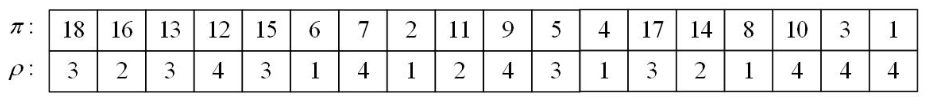
The pre-solved problems of the scheme proposed in this paper involves the sub-problem of operation arrangement and the sub-problem of machine selection. Therefore, in this paper, we apply the individual representation method to the double chain, that is, use the process chain and the equipment chain to jointly represent the individuals in the population, as shown in Figure 2. For the sub-problem of operation arrangement, we use the operation chain π to represent it, that is, π(i) means that the process O_π(i) is ranked in the ith position of the process chain. For the sub-problem of machine selection, we use machine chain ρ to represent it, that is, ρ(i) indicates that the operation O_i is processed on the machine ρ(i).

3.2. Encoding

In this paper, we use the idea of reverse scheduling to pre-schedule the complex products. Therefore, for a tree that can display the product processing process, the root node indicates the beginning of scheduling, and the completion of all leaf nodes indicates that the product has been scheduled. Firstly, aiming at the sub-problem of operation scheduling, that is, the arrangement of each operation on the operation chain π, this paper proposes a real-time coding method using the process set on the root node. The coding process includes the following four sub-processes:

Step 1: Obtain the current root node operation set. Initially, the root node operation set has only one element, that is, the root node process;

Step 2: Obtain the current operation to be scheduled, that is, randomly select a root node from the current root node operation set for scheduling;

Step 3: Update the current root node process set, and add the processes in the child nodes of the currently selected process to the root node process set;

Step 4: Determine whether the process set of the root node is empty, if it is empty, it indicates that the process chain coding is completed, otherwise, skip to Step 1.

For the processing equipment corresponding to each process, this paper adopts the idea of roulette selection strategy. When a device takes less time to process a product, it is more likely to be used next. Through the above two steps, we can encode a complex product into a reasonable and feasible individual, and Figure 3 is an example of encoding for the product shown in Figure 1.

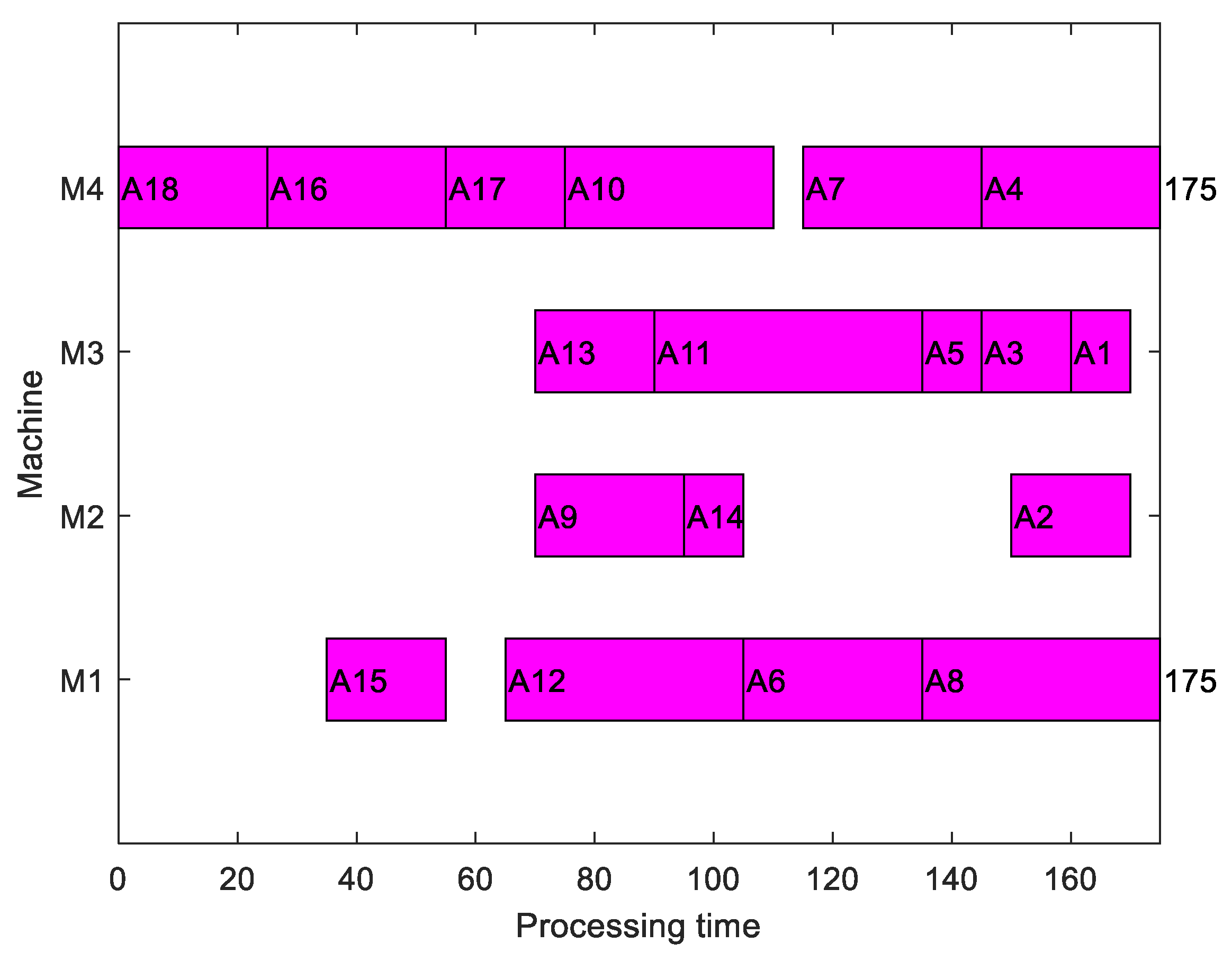
3.3. Decoding

For any individual in the population, this paper proposes a decoding method that applies the earliest possible start processing time to the decoding process to decode the individual into a specific scheduling scheme. Since the operation chain π specifies when the process should be scheduled, the machine chain $\rho$ specifies the processing machine corresponding to the operation. Therefore, we obtain each operation in turn from left to right and obtain the corresponding machine. Therefore, we obtain each process in turn from left to right and obtain the processing equipment corresponding to the process. Then, in the order from the first idle time to the last idle time, each process is processed at the earliest in the corresponding equipment. The detailed decoding steps designed in this paper are as follows, and a specific example is shown in Figure 4.

Step 1: Obtain the attribute information of operations, and set the pre-start processing time $p\text{\_}{s}_i$ of the process $O_i$ to 0, where $1\le i\le n$.

Step 2: Read a process gene in the process chain sequentially from left to right, set the process corresponding to this gene as $O_i$, read the equipment chain to obtain the processing equipment corresponding to this process as $M_k$, and the processing time as $t_{ik}$, $D_{i,j}$ is the migration time for transporting process O_i from its processing equipment to the processing equipment corresponding to O_j.

Step 3: Calculate the time when the actual processing operation of the operation O_i starts and the time when the processing operation ends. Find each idle time on the equipment $M_k$ in the order from the first idle time to the last idle time, that is, [$t_s$, $t_e$], and then compare the idle time with the time required for the process to be executed, if $\max \left(p\text{\_}{s}_i, t_s\right)+t_{ik}\le t_e$, so that the actual start processing time $S_i=\max \left(p\text{\_}{s}_i,t_s\right)$ of process $O_i$, otherwise, continue to compare the next idle time with the time required for the process to be executed. If the process execution condition is not met until the last idle time, the process will be executed on the device after other processes are executed. At this time, $S_i=\max \left(p\text{\_}{s}_i, c_k\right)$, where $c_k$ is the time when the last process on the device $M_k$ ends. The time $C_i=S_i+t_{ik}$ at which the execution of the actual machining operation of the operation $O_i$ ends.

Step 4: Reassign the pre-start processing time of the next process to be executed after process $O_i$. Read the product process partial sequence relationship table to obtain the next process to be executed after the process $O_i$. Assume that the next process to be executed after the currently acquired process O_i is O_j, then the pre-start execution time of the reassigned process O_j $p\text{\_}{s}_j=\max \left\{p\text{\_}{s}_j, C_i+D_{i,j}\right\}$, where $D_{i,j}$ is the migration time for transporting process $O_i$ to the equipment corresponding to process O_j.

Step 5: Judge whether the reading of the chromosome is completed. If the reading is completed, the decoding process ends and the product processing process is completed; otherwise, skip to Step 2.

3.4. Selection Method

We use a tournament selection strategy to select two parent chromosomes that participate in evolution, and the individual with the smallest completion time is selected as the parent chromosome. At the same time, the elite retention strategy is applied in the algorithm, so that the optimal individual at this stage is directly selected into the next generation population.

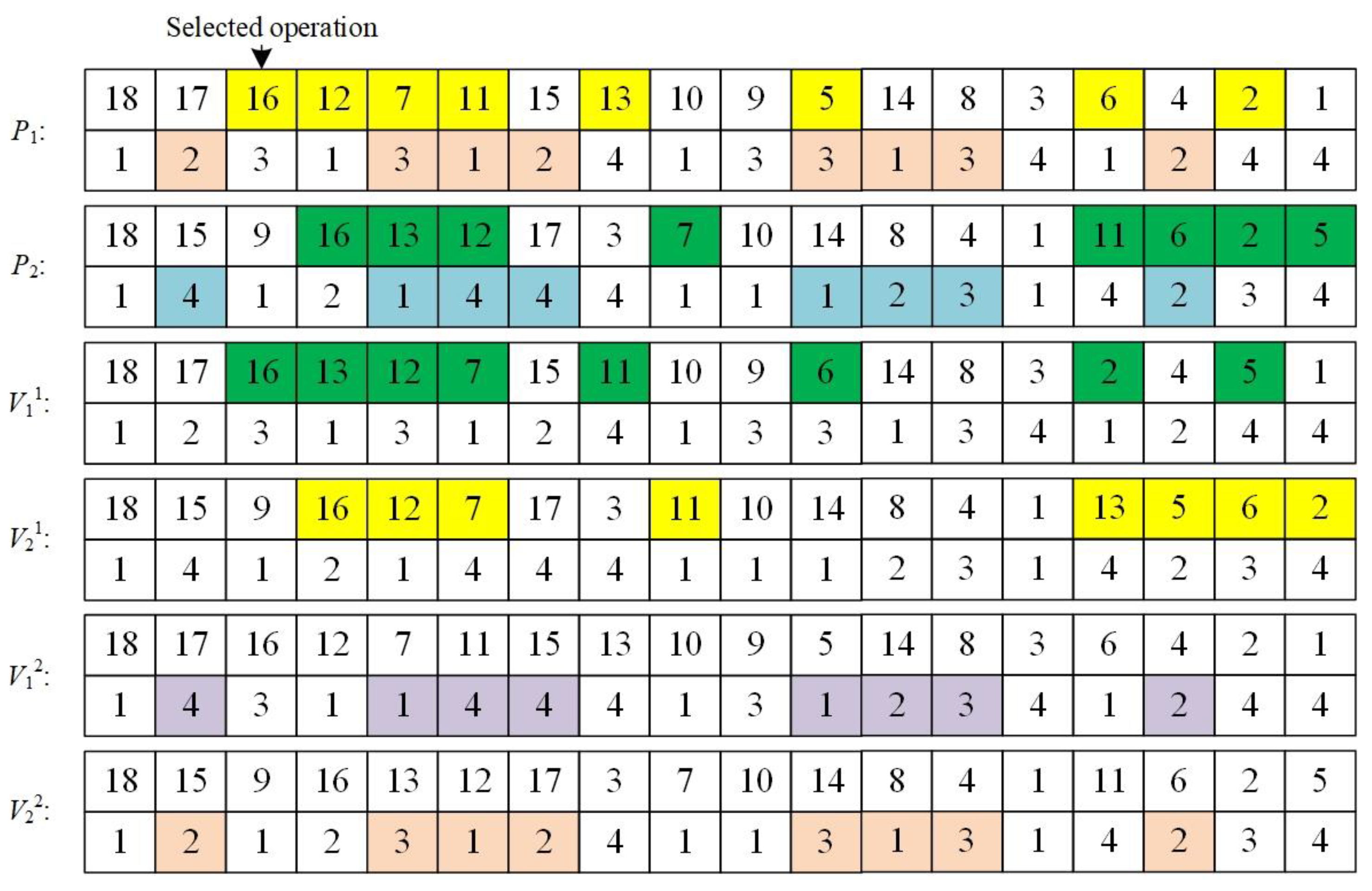
3.5. Crossover Method

In this paper, we adopt the crossover strategy of generating four-children, that is, generating four child chromosomes from two parent chromosomes. Based on position and operation, we give two crossover methods, namely the multi-child crossover method based on crossed row vector and the multi-child crossover method based on subtree. The algorithm randomly executes the above two crossover strategies during the execution process. If the number of chromosomes in the population reaches the individual maximum value, the crossover process is terminated. The detailed process of the implementation of the two crossover methods is as follows.

(1)

Multi-child crossover method based on crossed row vectors

Step 1: Two parent chromosomes involved in evolution are generated by the selection strategy described in this paper, assuming that the selected parent chromosomes are P₁, P₂;

Step 2: Randomly generate a 0–1 sequence with the same length as the chromosome operation chain as the recombination marker, 0 indicates that the position is not recombined, and 1 means that the position is recombined;

Step 3: Generate child chromosomes $V_1^1, V_2^1, V_1^2, V_2^2$ from the parent chromosomes P₁ and P₂ respectively, and the specific generation method is as follows.

(a) Generation of child chromosome $V_1^1$: The machine chain of the child chromosome $V_1^1$ is completely inherited from the machine chain of the parent chromosome P₁, and in the process chain, how to arrange the process on which the recombination flag bit is 1 is specified by the parent chromosome P₂, and the sequence of operations on the recombination flag bit 0 is exactly the same as that in the parent chromosome P₁. The specific crossover method of the operations that needs to be recombined in the operation chain is: obtain the recombination gene sequence corresponding to the process corresponding to the position where the recombination flag bit is continuously 1, and the gene in the recombination sequence is placed in the gene corresponding to the position of the process chain in the child chromosome $V_1^1$, and the placement order is specified by the parent chromosome P₂. The recombination string corresponding to other continuous recombination markers is obtained in turn, and the recombination is carried out in the above way to generate the final individual.

(b) Generation of child chromosome $V_2^1$: The machine chain in the child chromosome $V_2^1$ is completely inherited from the machine chain in the parent chromosome P₂, and the ordering of the procedures with the operations on the recombination flag bit 1 in the operation chain is specified by the parent chromosome P₁, and the recombination The sequence of the processes on the flag bit 0 is exactly the same as that in the parent chromosome P₂. The specific recombination method of the operations that needs to be recombined in the process chain is: obtain the recombination gene sequence corresponding to the process corresponding to the position where the recombination flag bit is continuously 1, and the gene in the recombination sequence is placed in the gene corresponding to the position of the process chain in the child chromosome $V_2^1$, and the placement order is specified by the parent chromosome P₁. The recombination string corresponding to other continuous recombination markers is obtained in turn, and the recombination is carried out in the above way to generate the final individual.

(c) Generation of child chromosome $V_1^2$: The operation chain in the child chromosome $V_1^2$ is completely inherited from the process chain in the parent chromosome P₁, and the machines corresponding to the operations whose recombination flag is 1 in the machine chain is designated by the parent chromosome P₂, the machine corresponding to the operation on which the recombination flag is 0 is exactly the same as that in the parent chromosome P₁. The recombination process of the machine chain is as follows: The operations corresponding to the positions where the recombination flag is continuously 1 is obtained as the new recombination gene sequence, and the processing machine required for each operation in the recombination string in the child chromosome $V_1^2$ is specified by the parent chromosome P₂, The recombination strings corresponding to the other consecutive recombination flags of 1 are sequentially obtained and recombined in the above manner to generate the final individual.

(d) Generation of child chromosome $V_2^2$: The operation chain in the child chromosome $V_2^2$ is completely inherited from the operation chain in the parent chromosome P₂, and the machine corresponding to the operation whose recombination flag is 1 in the machine chain is designated by the parent chromosome P₁, the machine corresponding to the operation on which the recombination flag is 0 is exactly the same as that in the parent chromosome P₂. The specific recombination method of the machine chain is as follows: The operation corresponding to the position where the recombination flag is continuously 1 is obtained as the new recombination gene sequence, and the processing machine required for each operation in the recombination string in the child chromosome $V_2^2$ is designated by the parent chromosome P₁. The recombination strings corresponding to the other consecutive recombination flags of 1 are sequentially obtained and recombined in the above manner to generate the final individual.

Figure 5 shows four child chromosomes generated by the above steps for two randomly generated parent chromosomes.

(2)

Multi-child crossover method based on subtree

Step 1: Two parent chromosomes involved in evolution are generated by the selection strategy described in this paper, assuming that the selected parent chromosomes are P₁, P₂.

Step 2: Randomly obtain all operations in a subtree as the current crossover operation string; Step 3: Generate child chromosomes $V_1^1, V_2^1, V_1^2, V_2^2$ from the parent chromosomes P₁ and P₂, respectively, and the specific generation method is as follows.

(a) Generation of child chromosome $V_1^1$: The machine chain in the child chromosome $V_1^1$ is completely inherited from the machine chain in the parent chromosome P₁. The sequence of each operation sequence of the crossover operation string in the operation chain is specified by the parent chromosome P₂, and the sequence of the remaining operations is exactly the same as that in the parent chromosome P₁.

(b) Generation of child chromosome $V_2^1$: The machine chain in the child chromosome $V_2^1$ is completely inherited from the machine chain in the parent chromosome P₂. The sequence of each operation sequence of the crossover operation string in the operation chain is specified by the parent chromosome P₁, and the sequence of the remaining operations is exactly the same as that in the parent chromosome P₂.

(c) Generation of child chromosome $V_1^2$: The operation chain in the child chromosome $V_1^2$ is completely inherited from the parent chromosome P₁. The machine corresponding to the process in the crossover operation string in the machine chain is designated by the parent chromosome P₂, and the machine corresponding to the remaining operations is exactly the same as that in the parent chromosome P₁.

(d) Generation of child chromosome $V_2^2$: the operation chain in the child chromosome $V_2^2$ is completely inherited from the parent chromosome P₂, the machine corresponding to the process in the crossover operation string in the machine chain is designated by the parent chromosome P₁, and the machine corresponding to the remaining operation is exactly the same as that in the parent chromosome P₂.

Figure 6 shows four child chromosomes generated by the above steps for two randomly generated parent chromosomes.

(3)

Analysis of the crossover method

In the above two methods, part of the operation chain or machine chain of the individual offspring is designated by another parent chromosome. Since the individuals in the population are all legal chromosomes, that is, the scheduling order between operations satisfies the priority constraint relationship, and the corresponding processing machine is also legal processing machine, the individuals generated by the above two methods are also legal individuals.

3.6. Mutation Method

(1)

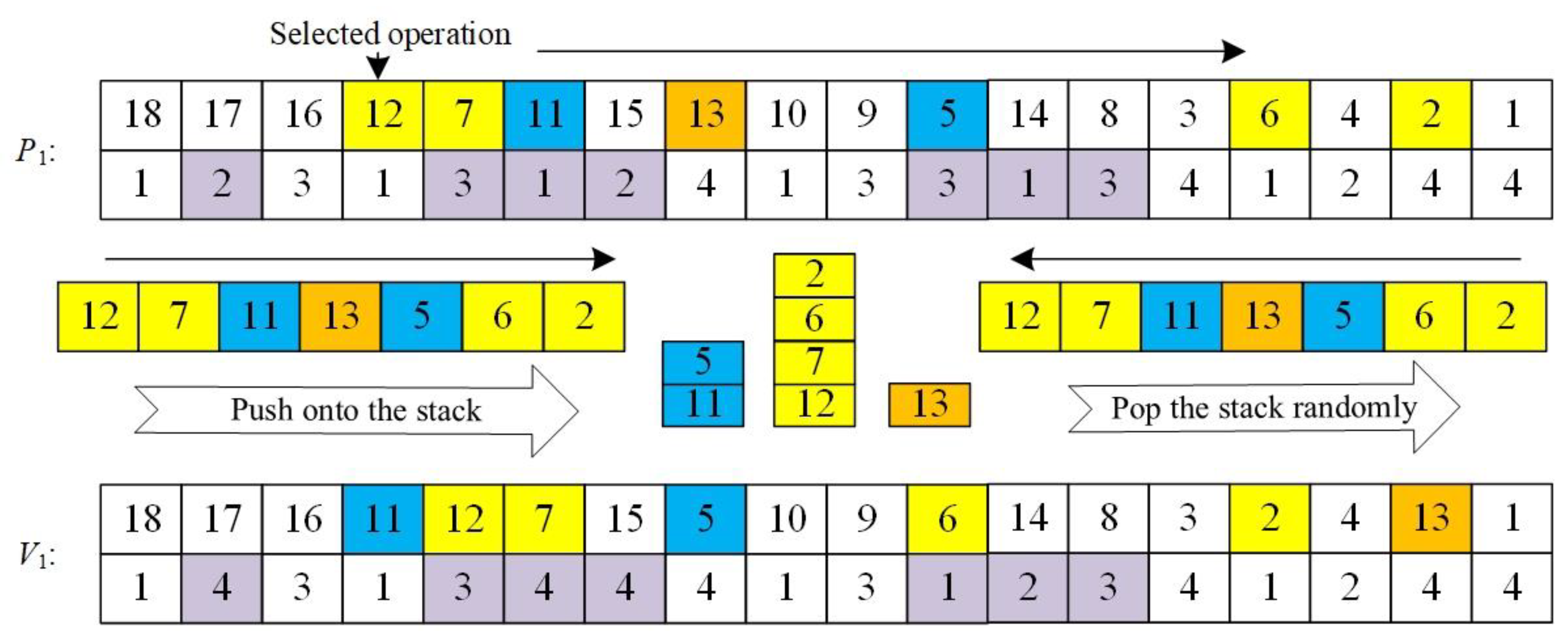
Chaotic mutation based on sibling operations

Step 1: Randomly select a process and its sibling operations, take each sibling operation as the bottom element of the stack, and add the descendant nodes of each sibling operation in the parent chromosome to its corresponding gene stack according to the order from front to back, so as to ensure that some processes in the same stack can be executed first under the influence of constraints, and the execution order of processes in different stacks will not be affected by constraints.

Step 2: Delete the selected operation and its corresponding processing machine in the parent chromosome.

Step 3: Randomly pop the top element of the stack and insert it into the last free position of the process chain in the child chromosome and re-determine which device should be processed for it according to the roulette selection strategy, repeat the above steps until all stacks are. If no element is present, it will no longer mutate.

An example of the encoding process of the encoding method introduced in this article is shown in Figure 7, wherein operation O₁₂, O₁₁ and O₁₃ are sibling operations.

(2)

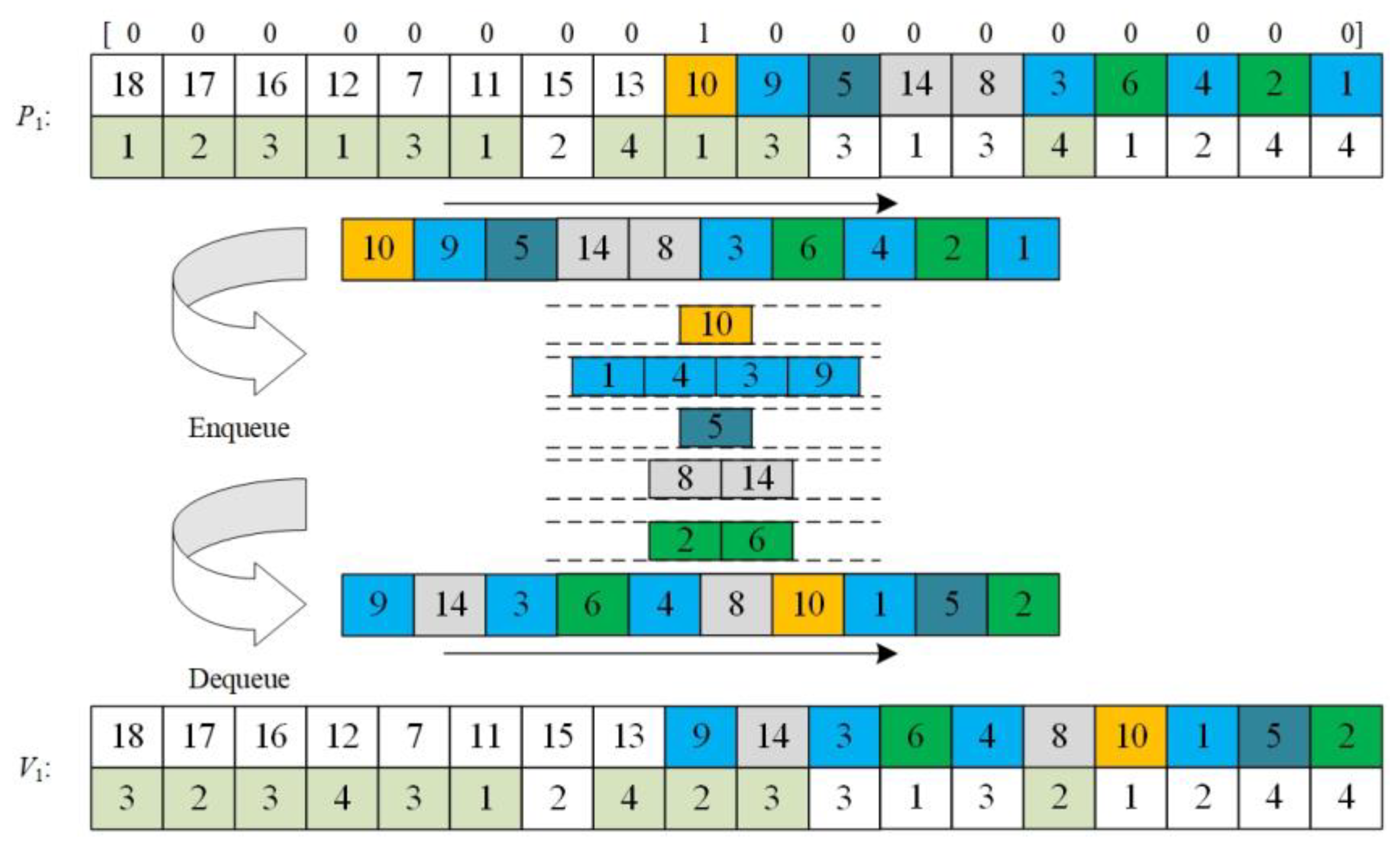
Random mutation based on mutation row vector

Step 1: Randomly generate a mutation row vector, in which the elements are 0 or 1, and there is only one 1, which is used to identify the mutation position, and the operation sequence after the mutation position is the mutation gene sequence.

Step 2: Put the processes in the mutant gene sequence into different queues from front to back, so that the processes in the same queue are affected by the constraints, and the processes not in the same queue are not affected by the constraints.

Step 3: Randomly dequeue elements in different queues to generate mutated operation substrings and select the processing machine for them according to the roulette selection strategy. Repeat the above steps and specify that all queues are empty, and the mutation no longer takes place.

Figure 8 is the process of producing new individuals by the above mutation method.

(3)

Analysis of the mutation method

In the above two mutation methods, the generation of the mutation string relies on stacks or queues, and the application of stacks or queues ensures that the operation of the final generated substrings satisfy the priority processing constraint relationship. Therefore, the two mutation methods designed in this paper will not produce infeasible individuals.

3.7. Local Search

This paper uses the local search method to increase the efficiency of the algorithm to retrieve the optimal solution better and faster. Specifically, to obtain the critical path corresponding to the optimal individual plan, first change the equipment corresponding to the process one by one in the order from the first process to the last process, then compare the advantages and disadvantages of the old and new scheduling plans, and finally retain the optimal plan as the latest scheme.

3.8. The Conversion Strategy Based on Completion Time Flipping

As the idea of reverse order scheduling is adopted in this paper, when an individual is decoded as a specific scheduling scheme, the generated Gantt chart is still in the form of reverse order. In order to obtain a positive sequence scheduling, we adopt the conversion strategy based on the completion time flipping [29] that we previously proposed. When the proposed conversion strategy is used to convert the scheduling scheme shown in Figure 4, the final positive scheduling scheme is shown in Figure 9.

3.9. Algorithm Process

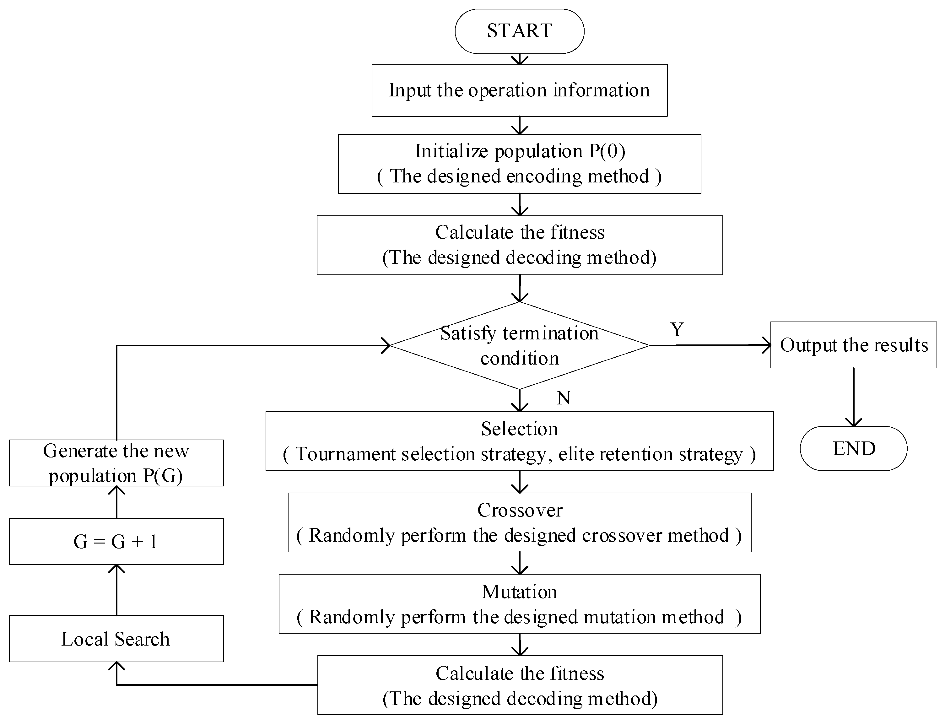
As shown in Figure 10, the algorithm designed in this paper randomly performs crossover and mutation operations during operation. If the objective function value corresponding to the optimal individual of the population is not improved in consecutive G generations, the algorithm terminates.

4. Experimental Results

In order to better demonstrate the advantages of the algorithm proposed in this paper, comparative experiments are set up in this chapter. We generated 100 calculation examples by randomly selecting parameters such as the number of processes and the amount of equipment. Among them, the value range of the number of processes is [50, 100], the value range of the number of equipment is [4, 8], the range of time consumed by the process moving between different devices is [1, 10], and the processing time of the process is [1, 20], the number of product process tree layers is [2, $\lceil n/2\rceil$], which is the number of processes in the current process tree.

4.1. Parameter Setting

This chapter adopts the Taguchi experimental design method to test which set of parameters makes the algorithm perform better [30]. Firstly, it is tested by using the calculation example I_85_5_1, 85_5, which indicates the running time and the size of the amount of data involved (n = 85, m = 5), and one indicates the first calculation example mentioned in this paper. There are four parameters that need to be focused on in this algorithm: Population size (Ps), crossover probability (Pc), mutation probability (Pm), G (If the current solution of the algorithm does not become better in consecutive G generations, then Algorithm execution stops). Four levels of impact factors are divided, and the combinations of different parameter values are shown in

Table 2. Each algorithm corresponds to the impact factor level.

Parameters	Factor Level
	1	2	3	4
Ps	n × 1	n × 2	n × 3	n × 4
G	10	20	30	40
Pc	0.6	0.7	0.8	0.9
Pm	0.1	0.2	0.3	0.4

. Select the orthogonal array L16(4⁴). For each different parameter combination, the algorithm needs to be run 30 times, and the average completion time obtained from 30 runs is taken as the experimental index. The final experimental results are shown in

Table 3. Orthogonal test results.

Experiment Number	Factor Level			Index
	Ps	G	Pc	Pm	Makespan Average
1	1	1	1	1	206.5
2	1	2	2	2	199.7
3	1	3	3	3	198.3
4	1	4	4	4	193.6
5	2	1	2	3	192.4
6	2	2	1	4	189.5
7	2	3	4	1	188.7
8	2	4	3	2	189
9	3	1	3	4	191.4
10	3	2	4	3	180.4
11	3	3	1	2	185.8
12	3	4	2	1	187.8
13	4	1	4	2	179.8
14	4	2	3	1	182.7
15	4	3	2	4	177.3
16	4	4	1	3	180.4
K1	798	770.2	762.2	765.7
K2	759.6	752.3	757.2	754.3
K3	745.4	750.1	761.4	751.5
K4	720.3	750.8	742.5	751.8
k1 = K1/4	199.51	192.55	190.55	191.43
k2 = K2/4	189.89	188.18	189.31	188.58
k3 = K3/4	186.36	187.52	190.35	187.88
k4 = K4/4	180.08	187.69	185.63	187.94
Range	19.43	5.03	4.92	3.55
Rank	1	2	3	4

. The changes of the experimental indicators affected by each parameter are shown in Figure 11.

According to Table 3 and Figure 11, the following conclusions can be drawn. First, by analyzing Figure 11, we can clearly observe that the parameter Ps has the most obvious influence on the algorithm among the four parameters. The value of Ps changes with the influence factor. When it increases, the average value of the experimental index also changes from 199.51 to 180.08, and the time required to complete the processing also decreases. It can be seen that the optimal value of Ps is n ∗ 4. The second one that has a more obvious impact on the algorithm is G. When the value of G increases with the change of the impact factor, the average value of the experimental index also changes from 192.55 to 187.52. When the G value is 30, the average time required for processing to complete is the smallest. Therefore, in this experiment, set G to 0.9. Then, the third parameter that affects the algorithm is Pc. When the value of Pc increases with the change of the impact factor, the average value of the experimental index changes from 190.55 to 185.63. Different from the first two parameters, with the increase of Pc, the time required for the completion of processing presents a trend of first decreasing, then increasing and then decreasing. When the value of Pc is 0.9, the time required for processing is the shortest. Finally, the parameter that has the least impact on the performance of the algorithm is Pm. When the value of Pm increases with the change of the impact factor, the average value of the experimental index changes from 191.43 to 187.88, and the range of change is 3.55. With the increase of Pm, the time required for processing to complete decreases first and then increases. When the value of Pm is 0.3, the average time required for processing to complete is the least. Through the above analysis, the optimal values of the four parameters of the algorithm described in this chapter should be: Ps = n ∗ 4, G = 30, Pc = 0.9, Pm = 0.3.

4.2. Comparative Experiment

We chose the comprehensive scheduling algorithm CPFS_CJ [9] with priority constraints, the chain scheduling algorithm LSA [31], the comprehensive scheduling algorithm CSA_VCLDC [23] using virtual component level partition coding, and the comprehensive scheduling algorithm based on process relationship matrix table coding ISA_ORMT [25] and ISA_DROS. In terms of the solution quality of the problem as a comparison, the above algorithms are respectively applied to solve the set of examples mentioned in this chapter. All algorithms are implemented by MATLAB programming, the operating environment is 64-bit Win10 operating system, the processor is Intel(R) Core(TM) i7-4810MQ [email protected], and the memory is 16G. The algorithm runs independently for each example in the test set 30 times. In this section, the solution quality and solution speed of the proposed algorithm are compared with those proposed by other researchers.

In the process of solving 100 calculation examples, for each calculation example, when each algorithm is run independently for 30 times, the minimum time required for the completion of product processing is shown in Figure 12, and the average completion time obtained is shown in Figure 13. It shows that most of the change curves of the minimum completion time and the average completion time of the algorithm ISA_DROS proposed in this chapter are located below the entire graph. Figure 14 summarizes the results in Figure 12 and Figure 13. The second set of data is the statistics of the average completion time results shown in Figure 13, in which the algorithm ISA_DROS obtains the optimal solution of 66 instances, the algorithm ISA_ORMT obtains the optimal solution of 22 instances, and the algorithm CSA_VCLDC can only solve 14 instances The optimal solution of the algorithm CPFS_CJ and LSA did not obtain the optimal solution. Since the algorithms CPFS_CJ and LSA are both rule-based heuristic algorithms, we only counted the average running time of several other comparative algorithms, as shown in Figure 15. It can be clearly concluded that the solving ability of the algorithm proposed in this paper is better than other comparison algorithms.

Figure 16 shows the completion time obtained by running the algorithms ISA_DROS, ISA_ORMT and CSA_VCLDC 30 times independently for a single randomly generated instance. Figure 17 shows the running time during the algorithm solution process. It can be seen from Figure 16 and Figure 17 that the algorithm ISA_DROS proposed in this paper is better than the other three algorithms.

5. Conclusions and Future Research

In order to solve the comprehensive scheduling problem faced by complex products with tree structure in the flexible equipment network scenario, this paper combines the genetic algorithm and dynamic scheduling algorithm to propose a reverse sequence equipment network comprehensive scheduling algorithm based on the dynamic root node process set. First, in order to facilitate the design of the algorithm, based on the idea of reverse order scheduling, a real-time encoding method using the root node process set is given to ensure the availability and excellence of the population individuals in the initial state. Then, two corresponding crossover and mutation methods are given by using position and operation, which ensures that infeasible solutions will not be generated in the process of population evolution and avoids the detection and repair of additional infeasible solutions. A simple decoding method using the earliest available completion time and the positive sequence conversion strategy of the optimal scheduling scheme is given. After comparing the algorithm with the algorithms proposed by other researchers, the algorithm has higher performance in obtaining feasible solutions and is more in line with the actual application scenario.

At present, there are still relatively few integrated scheduling solutions based on intelligent optimization algorithms, and the integrated scheduling problems involved are still limited. Therefore, in the future, we can try to introduce other intelligent optimization algorithms into the processing of comprehensive scheduling problems. This article does not consider the problem that multiple products are processed concurrently, and the order arrival event cannot be accurately determined in the process of dealing with the problem. Therefore, in the next research work, a more reasonable solution should be designed to solve this problem.