Self-Supervised Health Index Curve Generation for Condition-Based Predictive Maintenance

Abstract

Modern machine degradation trend evaluation relies on the unsupervised model-based estimation of a health index (HI) from asset measurement data. This minimizes the need for timely human evaluation and avoids assumptions on the degradation shape. However, the comparability of multiple HI curves over time generated by unsupervised methods suffers from a scaling mismatch (non-coherent HIs) caused by the slightly different asset initial conditions and distinct HI model training. In this paper, we propose a novel self-supervised approach to obtain HI curves without suffering from the scale mismatch. Our approach uses an unsupervised autoencoder based on a convolutional neural network (CNN) to detect initial faults and autonomously label measurement samples. The resulting self-labeled data is used to train a 1D-CNN health predictor, effectively eliminating the scaling mismatch problem. On the basis of a bearing test-to-failure experiment, we show that our self-supervised scheme offers a promising solution for the non-coherent HI problem. In addition, we observed that our method indicates the gradual wear affecting the bearing prior to the independent analysis of a human expert.

1. Introduction

The accurate monitoring of a machine’s degradation plays a pivotal role in condition-based predictive maintenance, facilitating timely maintenance actions and maximizing the lifespan of critical assets [1]. Contemporary assets are monitored by several sensors in order to detect potential defects at an early stage and estimate the remaining useful life (RUL) of the asset. Typically, the machine deterioration is assessed by evaluating a so-called health index (HI). A HI is a numerical value derived from the raw data samples for each measurement of the monitored asset. It is intended to reflect the health status of the system.

If evaluated over time, this so-called HI curve develops either an increasing or decreasing slope. The direction of the trend is depending on the HI definition. In conventional condition monitoring, this definition is based on the assessment of a device maintenance expert [2]. Hence, the HI is constructed by evaluating relevant trending parameters from a range of possible features [3] to monitor the device’s health. Typically, RUL is then assessed by comparing HI curves of multiple devices [4]. However, the approach depends on prior knowledge about the potential faults in the monitored device to select the correct parameters, as individual features may only be relevant to certain types of faults. This time-consuming, expert-guided selection may therefore suffer from a human-induced bias that limits their general applicability to a wider range of potential problems.

To counteract the human selection bias, more extensive HI estimation approaches have emerged. These either construct the HI based on autonomous evaluation of multiple traditional features [5] or use data-driven supervised learning methods to extract expert-independent features from the raw data [6]. Supervised machine learning methods have been heavily used in predictive maintenance [7,8,9,10].

Nonetheless, these methods necessitate a certain degree of human domain expertise. For instance, supervised methods require sets of labeled data, which are initially generated through time-consuming expert assessment. Thus, the extensive data volumes required to effectively train these supervised models present operational challenges. In addition, these methods make assumptions about the degradation shape [11], which do not hold in real-world scenarios, emphasizing the necessity for more efficient domain knowledge-independent approaches. In the remainder of this paper, we introduce a novel methodology that eliminates the need for human labeling in the context of HI generation and operates without making any assumptions regarding degradation shape.

2. Related Literature, Problem Statement and Contribution

In recent advancements, unsupervised learning-based HI methods based on autoencoders are proposed in order to minimize time-consuming human evaluation of the individual measurements and eliminate assumptions about the degradation of the asset [12]. Autoencoder are trained to reconstruct given input through an architecture bottleneck, the so-called latent vector. By training a reconstruction task, these models are expected to learn valuable features of the process of generating the data without requiring label information. Autoencoders are related to transformer networks [13], which are state-of-the-art models in many sequence-related tasks such as language translation or time-series forecasting. However, transformers require unsupervised training on large datasets, which is not available in many predictive maintenance scenarios. For this reason, recent studies mostly leverage unsupervised autoencoder approaches based on long short-term memory (LSTM) [14] or convolutional neural network (CNN) [15].

In the context of unsupervised HI curve generation, the autoencoder is trained exclusively on healthy unlabeled measurements of a monitored functional device, which is usually present at the beginning of a test-to-failure experiment. As depicted in Figure 1, the HI curve generation is centered around the idea that any autoencoder output, trained solely on healthy data, achieves worse reconstruction results as the wear-induced signal changes, which were not present in the training data, emerge over time. Therefore, the autoencoder HI is supposed to increase as the device is affected by wear over time.

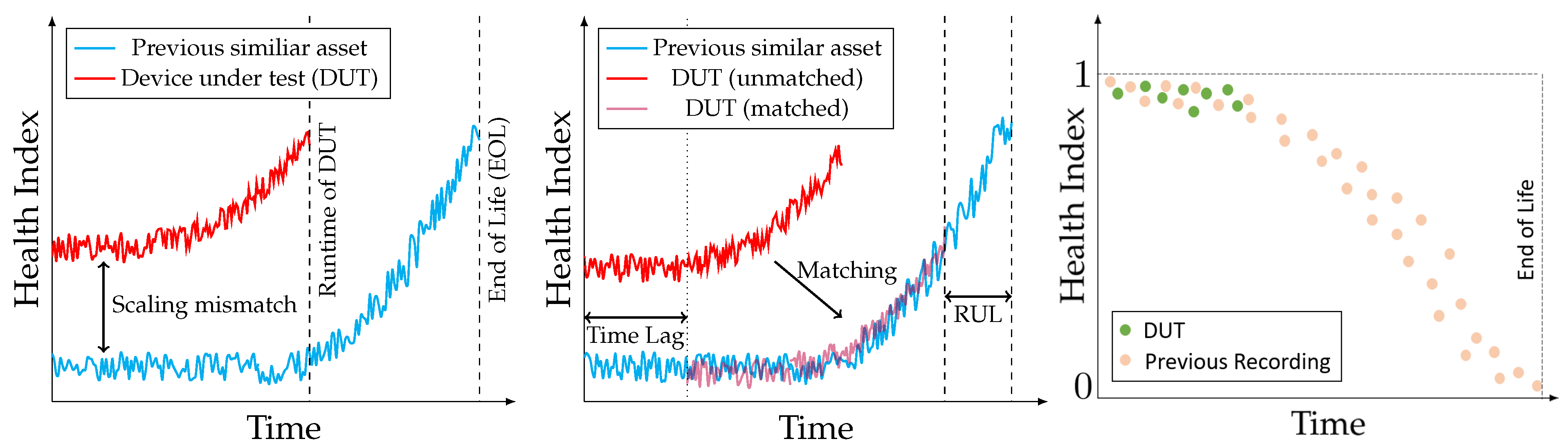
Previous work provided evidence that unsupervised HI curves based on autoencoders can be used to achieve state-of-the-art RUL estimation performances [16]. In this work, the RUL is determined by matching HI curves from devices under test (DUT) with pre-recorded curves derived from historical data of a similar asset by minimizing their Euclidean distance between the individual curves [17]. However, deriving the RUL of a device based on HI curves that are generated by unsupervised methods suffers from various limitations that we aim to address. Firstly, the initial value of the functional device is different for each individual machine. As stated above, any subsequent RUL estimation typically requires the comparison of multiple HI curves. Therefore, RUL estimation based on unsupervised HI evaluation is affected by a scaling discrepancy between individual curves, even when monitoring similar assets. An illustration of the scaling mismatch and the traditional matching-based RUL estimation is depicted in Figure 2.

This non-coherent behavior of unsupervised HI curves is typically explained by the influence of slightly different device initial conditions [12,18]. For this reason, recent RUL methods introduce a time shift variable, the so-called “time lag”. However, the real initial conditions of the DUT are unknown in practical application, compromising the accuracy and reliability of the RUL estimates of the method.

Secondly, to make the HI definition more intuitive, it is desirable for any HI curve to start with an initial health of 1 and to decrease over time, tending towards 0 as the device becomes worn out. This is indicated in Figure 2(right). Without additional time-lag estimation-based post-processing, this has not been implemented in autonomous HI generation [5,12,19].

To address these limitations, we propose a novel approach to HI generation based on self-supervised learning. Self-supervised learning has shown superior performance in data-heavy domains such as medical imaging [20] and general pattern recognition tasks [21]. Recently, self-supervised learning has been introduced to the field of condition monitoring and failure diagnosis to detect specific faults in electric powertrain data by using unsupervised support vector machines [22]. Unlike conventional supervised approaches, self-supervised methods do not require human-labeled data to train meaningful models. Instead, these methods aim to generate their own so-called ‘weak labels’ by evaluating unlabeled training data [23,24]. Note that in the literature, any label generated by a non-human expert is referred to as a weak label.

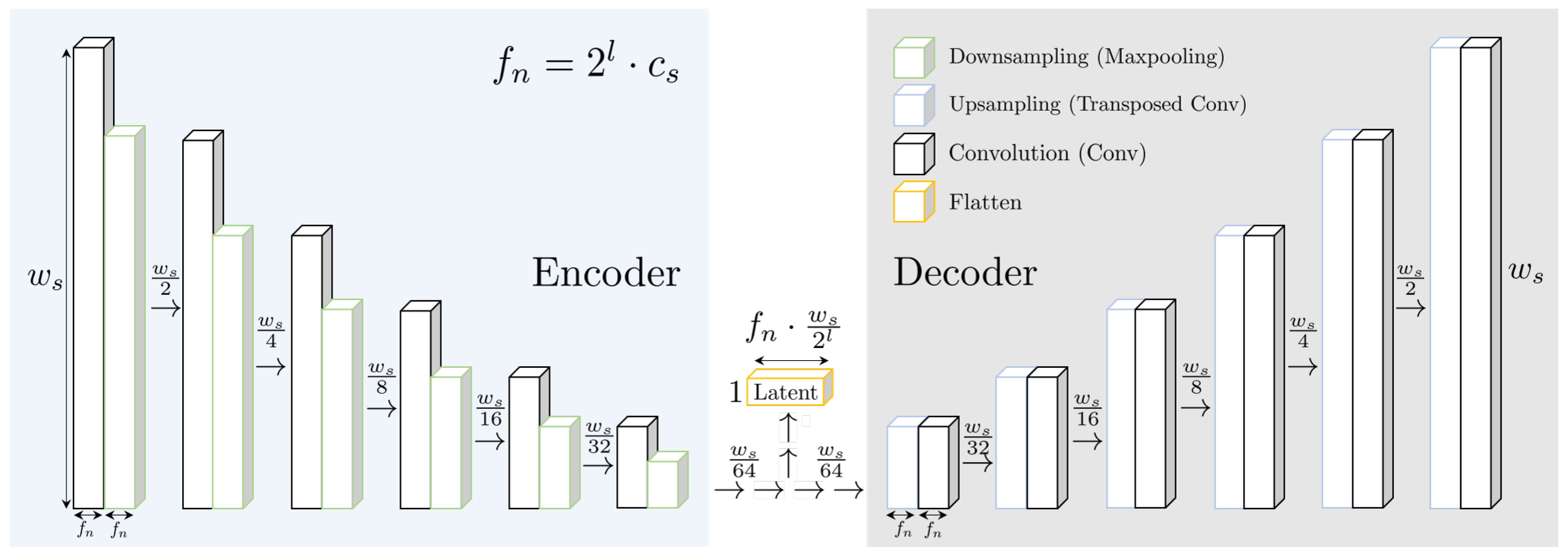
As illustrated in Figure 3, our method is based on a three-step appraoch: First, an autoencoder is going to learn an unsupervised representation of a data-generating process. Second, the trained model is used to detect the initial fault in the test-to-failure dataset. The initial fault, which is described in detail in Section 3.1.4, is used to provide weak preliminary labels for each measurement in a test-to-failure dataset by assigning individual measurements to either the ‘functional’ or ‘faulty’ class. Third, the weakly labeled data is used to train a subsequent two-class classifier generating the HI in a binary classification setting.

To the best of our knowledge, self-supervised learning remains unexplored in the context of HI curve generation and it provides a valuable contribution to the current literature on HI generation. This paper shows:

• The capability of self-supervised learning to estimate coherent HI curves of a device.
• The enhanced self-supervised HI performance of CNN- over LSTM autoencoder.
• That self-supervised HI curves indicate wear in the device prior to human experts.
• The effects of imperfect weak labels on our proposed self-supervised HI method.

The rest of the paper is organized as follows: The proposed method is explained in Section 3. The experimental setup used for verification is introduced in Section 4 and the main results are presented in Section 5. Section 6 concludes this article.

3. Methods

3.1. Generating Unsupervised Weak Labels Applying Autoencoder

3.1.1. Data Preprocessing

Our autoencoder is trained on a set of unlabeled measurements of a functional device recorded in a test-to-failure experiment. Each experimental run contains multiple unlabeled measurements $X=\left\{x\right(1),x(2),\dots ,x\left(i\right),\dots ,x(L\left)\right\}$ of the device. Each of these measurements is a time-series of length of L and each point $x\left(i\right)$ is a regular sensor reading at time-instant i of the recording. For training, we only use measurements taken after an initial run-in period of 15 min to bypass any short-term transient behavior. In addition, we solely rely on the first hour of the remaining available test-to-failure data. This ensures that the autoencoder is trained only on healthy data. Every individual measurement X is then split into multiple smaller sample windows of vector size $w_s$. Every $x\left(i\right)$ in this vector is re-scaled in the interval $[0,1]$ in advance, to speed up the training process. These scaled input data vectors (sample windows) are shuffled and fed sequentially into the input layer of the autoencoder.

3.1.2. Autoencoder Topologies

Autoencoder topologies consist of an encoder and a decoder. Both are connected by the so-called latent vector. While the encoder is supposed to compress the information into the latent, the decoder uses the latent to reconstruct the output. To prevent a trivial result and learn an unsupervised model of the monitored device, compression on the encoder side is achieved by reducing the size between the consecutive layers in the encoder. Therefore, the connecting latent represents an information bottleneck, which is supposed to contain essential information about the data-generating process. Our proposed CNN autoencoder architecture is depicted in Figure 4.

The CNN performs a discrete convolution of the input signal with a so-called kernel to extract related features from the data. We decided to utilize this network type due to its computational power, simple implementation, and success in similar predictive maintenance problems. The encoder topology of our network is based on six layers of 1D convolutions (Conv). This total amount of layers in the encoder is denoted by l. Convolutional layers are typically made of multiple kernels, the so-called feature maps. They contain the neural network weights ${\theta }_k$. The kernel size $k_s$ is typically smaller than $w_s$ in order to enable step-wise sliding of the kernel. Moreover, the sample windows are padded, using zero values at the start and end of each window.

In every convolutional layer, a kernel of size $k_s=3$ continuously slides over the sample window with a stride of zero and calculates the dot product between the input vectors window and the kernel weights ${\theta }_k$. Subsequently, a trainable bias $b_o|\{o=0,1,2,\dots ,l\}$ is added, and the result, processed by a nonlinear activation function (ReLU), is stored in the activation map. In the six similarly structured deconvolution layers (deconv) of the decoder, this process is reversed by performing transposed convolutions. The outputs given by the last decoder layer are called the reconstruction $R=\{\mathbf{r}(1,{\theta }_k),\mathbf{r}(2,{\theta }_k),\dots ,\mathbf{r}(i,{\theta }_k),\dots ,\mathbf{r}(w_s,{\theta }_k)\}$. Each conv or deconv layer is followed by a max-pooling/upsampling layer to halve/redouble the data dimensionality and adjust data resolution. Therefore, the information in the input vector of size $w_s$ is compressed with a loss based on the number of layers l until reaching the bottleneck at the latent of the autoencoder. To enhance the comparability of different architectures the number of feature maps $f_n$ trained within a single network layer is set to $f_n=2^l·c_s$. The compression ratio $c_s$ is calculated between the latent vector of size $s_{\mathrm{la}}$ and the input window size $w_s$ by $c_s=\frac{s_{la}}{w_s}$. Adopting the number of feature maps $f_n$ ensures the size of the flattened latent vector $s_{\mathrm{la}}$ to be $s_{la}=w_s·c_s$. Therefore, a desired compression ratio between the input and the latent is reached for a fixed number of layers so that the learning task is always at the same level of difficulty.

As previously stated, the encoder and decoder can be constructed using various neural network structures such as CNN or LSTM. Therefore, we compare our CNN autoencoder architecture to the LSTM-based work of Malhotra et al. [14] for the weak labeling task. This model is a state-of-the-art anomaly detection algorithm used in many time series-related applications. However, we do not provide any additional implementation details of this LSTM network, since it is covered in detail within the comprehensive work of the authors.

3.1.3. Autoencoder Optimization Details

To learn from the given data samples, our 1D-CNN approach optimizes the error between the input value $x\left(i\right)$ and its individual reconstruction $r\left(i\right)$ after passing the network. This error is summed for $w_s$ timepoints within the sample window. We received the reconstruction error

$$E_{}\left({\theta }_k\right)=\sum _{i=0}^{w_s}{\parallel x\left(i\right)-r(i,{\theta }_k)\parallel }^2$$

(1)

for each window. To obtain a trained model, we optimize each network parameter ${\theta }_k$ n order to derive the set of best weights characterized by

$${\tilde{\theta }}_k=\underset{{\theta }_k}{arg\; min}{E}_{me}\left({\theta }_k\right)$$

(2)

that minimizes $E_{me}$, which is the averaged sum of individual sample window errors $E_{}\left({\theta }_k\right)$. The optimization was performed using ADAM, which computes an adaptive learning rate for each individual weight of the network. The initial learning rate $\lambda$ was set to $\lambda =0.002$ at the start of the optimization. After successful training, the autoencoder is expected to achieve a suitable reconstruction performance on the data of the functional device.

3.1.4. Reconstruction Error-Based Generation of Weak Labels

As depicted in Figure 5, the initial fault is the first indication of wear in the device. It is estimated by sequentially feeding the remaining unlabeled data, which is not used to train the autoencoder, into the trained model. Then, $E_{\mathit{me}}$ is evaluated for each measurement of the test-to-failure experiment. If $E_{\mathit{me}}$ succeeds a given threshold for the first time an initial fault is present in the data. All remaining measurements after the initial fault are labeled as ‘faulty’, while the previous data samples are labeled ‘functional’. The decision threshold required to estimate the initial fault can be determined by various change-point detection-based methods [25], their individual evaluation is out of the scope of this work.

3.2. Self-Supervised HI Generation Using Weakly Labeled Data

In order to obtain our proposed self-supervised HI, the weakly labeled data are used to train a binary classification model to decide whether the bearing is still working (‘functional’) or is affected by severe wear (‘faulty’) over time that prohibits further use of the machine. Note that, as explained in Section 3.1.1, we trained the autoencoder on data measurements of a functional device after a period of 15 min since we desire to bypass any transient run-in behavior. Any run-in and autoencoder training data are not used to train the HI classifier. Additionally, we do not train the self-supervised HI model on data of the final failure. These data originate from a machine that is completely worn out, thus no longer depicting a gradual deterioration of the system but rather reflecting the consequences of a specific complex fault type. The behavior in the final failure state is often very different from the behavior exhibited as the machine progresses towards it. Thus, we exclude these data from the trainset. The architecture of the classifier is shown in Figure 6.

The feature extraction of the model is based on a 1D-CNN with three convolution and pooling layers. The outputs are fed into a single 100-neuron perceptron layer followed by a softmax decision layer to perform the binary classification task. The parameters of the model are trained by minimizing the cross-entropy $J_i$:

$$\underset{{\theta }_g}{arg\; min}{J}_i(t_{i,j},y_{i,j})=\underset{{\theta }_g}{arg\; min}\left(-\sum _{j=0}^{N_{cl}-1}{t}_{i,j}\log \left(y_{i,j}\right)\right)$$

(3)

between the prediction of the classifier $y_{i,j}$ and the generated preliminary labels $t_{i,j}$. Here, j corresponds to the j-th class, $N_{cl}$ to the number of classes and i to the time point. By definition, $N_{cl}$ equals 2 in the case of binary classification. Analog to the unsupervised autoencoder, we use the Adam optimizer to obtain the parameters of the classifier. The self-supervised HI is then determined by evaluating the results of the trained classifier. In this process, the class probability that each measurement originates from a functional device is calculated. Due to the design of this binary classification, the predicted bearing state of the HI is numerically bounded between zero (faulty) and one (functional).

4. Experimental Setup and Evaluation Metrics

4.1. Dataset Description

In our work, we assess the proposed self-supervised scheme through a comparative data analysis of two identical roller bearings subjected to test-to-failure experiments. To validate the effectiveness of our method, we utilized the test rig depicted in Figure 7.

The test rig was equipped with four ‘SONOTEC T10’ broadband ultrasound (US) sensors. To capture sensor data, the signals were analog-to-digital (A/D) converted using a 24-bit A/D converter with a maximum sampling rate of 204 kHz. To expedite the dataset generation process, we imposed a relatively short bearing lifetime by subjecting the test bearing and the gear connecting the shafts to a constant load of 1000 Nm. To ensure consistency, the rotational speed was maintained at 2000 RPM throughout all experiments. In each test-to-failure experiment, we recorded a 10-s measurement every 10 min (for bearing 1) and 5 min (for bearing 2) until the device failure was evident to the expert. A total of 3188 individual measurements were conducted, with each measurement evaluated by a human expert to provide the ground truth labels used in our experiments. The ground truth analysis involved examining the commonly used spectral envelope feature of the measured signal.

4.2. Comparison of Different Weak Labeling Architectures

As explained in Section 3.1.4, initial faults can be identified using different change-point detection methods. The accuracy of the initial fault detection depends on the quality of the deterioration trend. However, in this work, we aim to evaluate the suitability of the proposed general self-supervised HI framework and an exhaustive analysis of specific threshold algorithms is out of the scope. Therefore, the deterioration trends generated by different autoencoder models are compared, assessing their general suitability for the binary HI classification task. Figure 8 illustrates our approach.

The autoencoder performance is assessed by varying a discrimination threshold and analyzing the Area Under the Receiver Operating Characteristic Curve (AUC) of the method. The required Receiver Operator Characteristic (ROC) curve is given by calculating the true-positive ratio (TPR) and false-positive ratio (FPR) of every possible threshold compared to a ground truth label given by an expert manually looking through the data. A higher AUC value corresponds to a more suitable deterioration curve since a subsidiary initial fault threshold algorithm can achieve a result close to the ground truth determined by a human expert.

5. Results and Discussion

5.1. Unsupervised Generation of Preliminary Labels

In this section, we carefully evaluate the quality of our proposed CNN autoencoder model trained using the functional data. In addition, we compare our method with the LSTM-based autoencoder of Malhotra et al. [14] in terms of its suitability in the context of generating weakly labeled data. Our proposed self-supervised architecture relies on successful weak labeling of the unlabeled test-to-failure experiment data. It is therefore necessary that our model trained on functional device data achieves sufficient reconstruction performance on unseen data of this type. In addition, significantly worse performance should be evident on measurements affected by wear.

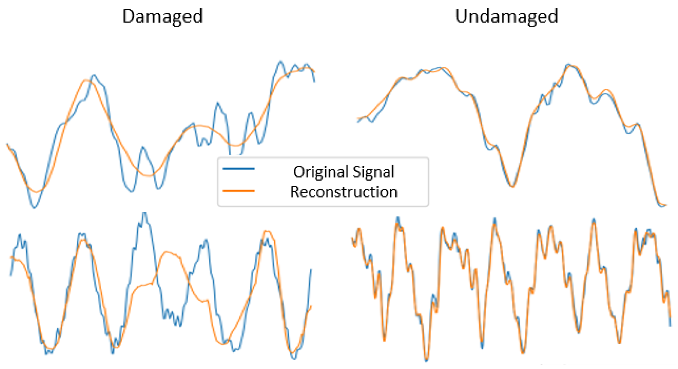
5.1.1. Evaluation of the Autoencoder Training Quality

Figure 9 shows normalized example reconstructions generated by our 1D-autoencoder for functional and faulty test signals.

Visually, the trained model achieves a suitable reconstruction performance for undamaged samples. However, it encounters challenges when reconstructing damaged data. As a result, the autoencoder appears to have learned an accurate model of the machine under normal operating conditions, which, as anticipated, proves less effective for data stemming from a degraded machine. In accordance with Section 3.1.4, we calculate the average autoencoder reconstruction error per measurement, denoted as $E_{me}$, over the entire operational life to estimate the initial faulty measurement within the deterioration curve of our test-to-failure experiments. 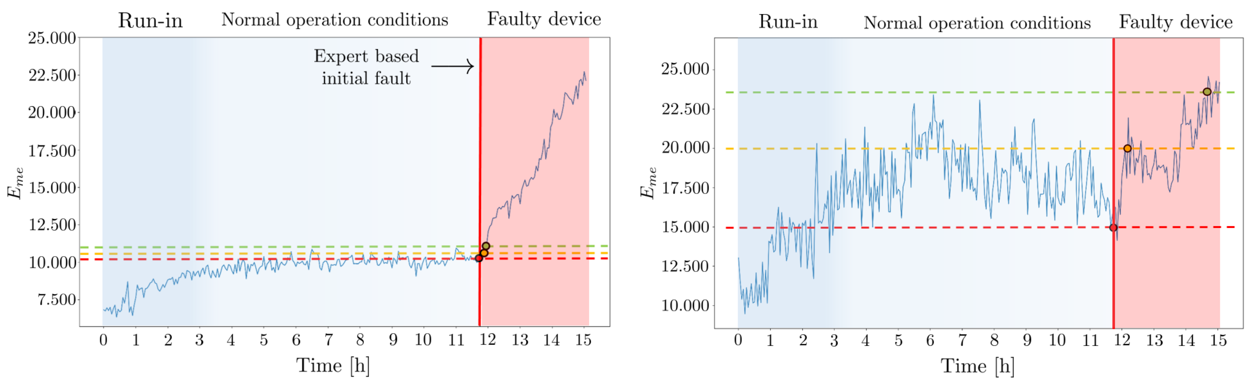Figure 10 illustrates the best deterioration curve achieved by the CNN and LSTM autoencoder on bearing 1. Additionally, the plot shows how the suitability of the deterioration curves is assessed with respect to Section 4.2.

Typically, early transient fluctuations usually do not reflect any real change in the health state of a time-worn machine under constant load. Thus, the dashed green line corresponds to an FPR of zero and marks the earliest possible correct initial fault estimate, not triggered early by random variations. In comparison, the dashed red line marks the ground truth threshold given by the human expert. The smaller the distance between both lines, the higher the AUC. Hence, a high AUC value indicates that the autoencoder model provides an initial fault estimation close to the human expert. Figure 11 presents the AUC-based comparison for both architectural models applied to bearing 1.

Despite skipping the first 15 measurements of the experiment, the results of both models seem affected by additional run-in effects, lasting until the 3-h mark of testing. The device transitions into a normal operational condition, maintaining it until the 12-h mark when it finally starts producing faulty data. As indicated by the green line, the optimal threshold of our CNN method lags behind the independent human expert’s initial fault baseline by approximately 15 min. In contrast, the best possible threshold for the LSTM-based curve lags by over 2 h. This distinction is also reflected in their respective AUC scores. While the CNN achieves an AUC of 0.98, the LSTM only attains an AUC of 0.78 with the best hyperparameter setting described in the original work. Consequently, our proposed CNN architecture significantly outperforms the LSTM reference from the literature. Comparable results were obtained for other test-to-failure runs on bearing 5. However, these results are omitted here for brevity.

5.1.2. Influence of the Input Vector Window Size $w_s$ and Compression $c_s$

The presented results of our CNN autoencoder are based on the choice of its hyperparameters, and for brevity, we only depicted the best performing so far. Nevertheless, we studied the impact of different input vector window sizes $w_s$ fed into our autoencoder and the influence of different data compression rates $c_s$ on the model performance. The results for both bearings within the dataset can be seen in

Table 1. AUC evaluation results of our 1D-CNN autoencoder for different $w_s$ and $c_s$.

	Bearing 1							Bearing 2
						Window Size $w_s$
Compression $c_s$	128	256	512	1024	2048	4096	6144	128	256	512	1024	2048	4096	6144
$50\%$	0.98	0.92	0.91	0.82	0.87	0.70	0.67	0.97	0.83	0.64	0.72	0.75	0.80	0.77
$25\%$	0.94	0.87	0.91	0.93	0.82	0.84	0.71	0.82	0.59	0.47	0.57	0.62	0.75	0.73
$12.5\%$	0.91	0.96	0.72	0.88	0.93	0.84	0.73	0.57	0.51	0.47	0.50	0.03	0.67	0.64
LSTM [26]	0.78	(best)						0.74	(best)

.

In our study, we achieve the best performance on both bearing test-to-failure runs using an input window size $w_s=128$ and a compression ratio $c_s=50\%$. Note that a window size of 6144 samples corresponds to a full rotation of the bearing. All other tested window sizes are derived from the power of two. They were chosen due to their frequent usage in the machine learning literature on CNN to support model comparability. We decided to only study sizes below a complete rotation, as this would lead to overlap between the individual windows, which would enhance the memory effect during training. The compression rates are determined to study the effect of a very strong (50%), medium (25%), and low (12%) compression level. Given that the best-performing model based on Malhotra et al. [14] using LSTM achieved inferior results compared to our best CNN model, all further evaluations are conducted exclusively with the CNN approach.

5.1.3. Visualization of the Trained Features Encoded in the Latent Vector

Related contributions on unsupervised HI estimation like [27] or [16] use visual evaluation methods like t-SNE [28] or PCA [29] to map the learned representations of the high dimensional latent vector onto a 2D plot and to compare the quality of different autoencoder models. Here, it is assumed that the most important information extracted by the trained autoencoder is present in its latent vector. By applying t-SNE and PCA, it is possible to explore emerging structures in this vector and to gain a deeper insight into results learned by a network.

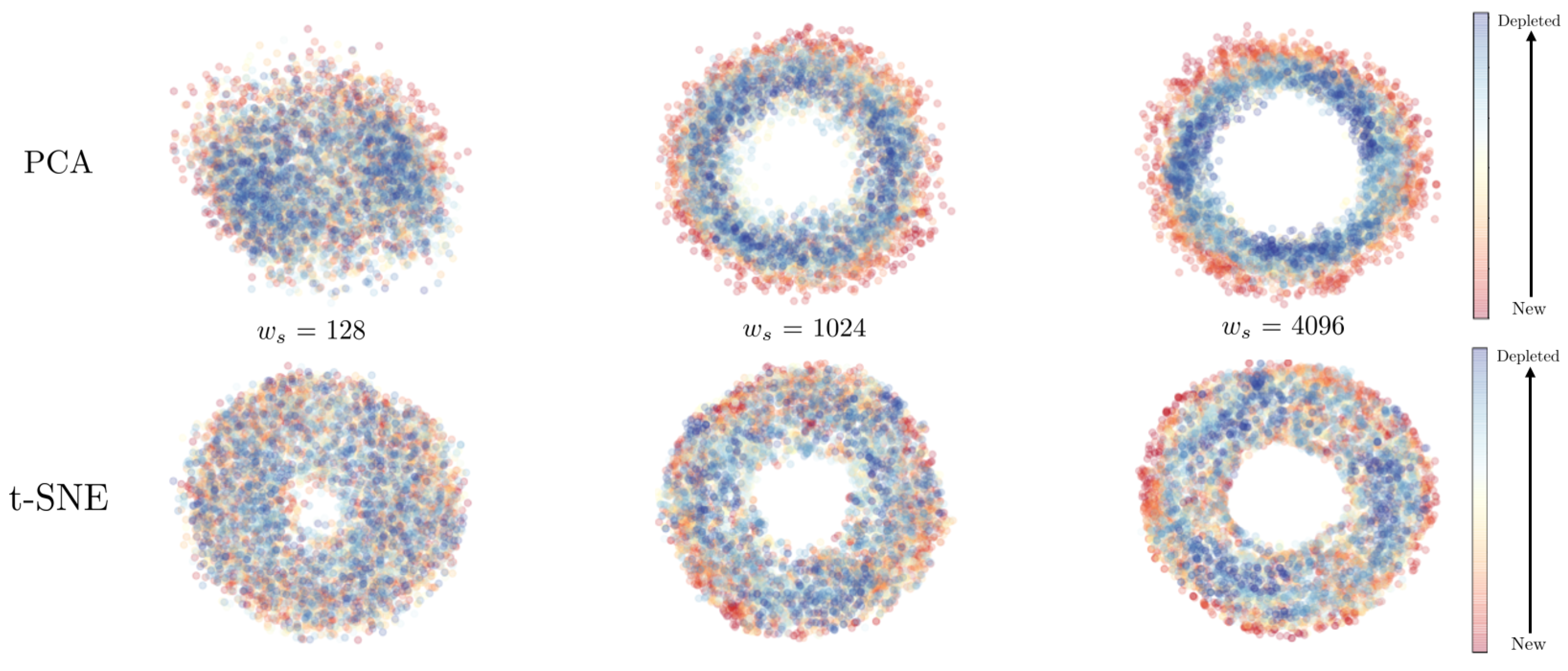
Figure 12 depicts such a t-SNE and PCA-based comparison of our CNN-autoencoder, using different window sizes and a fixed compression rate of 50%.

In the illustration, every individual point corresponds to a single measurement of the test-to-failure experiment for bearing 1. To achieve the plot, first, each measurement was fed sequentially into the trained autoencoder and the corresponding latent values were concatenated. Second, t-SNE and PCA were applied to the constructed high dimensional latent value matrix to map it to the depicted 2D plot. The recording period of each measurement is encoded by a colored gradient to visualize the chronological order of the recorded bearing life-cycle. Notably, both visualization methods yield toroidal representations that analyze the data of the rotating machinery. The results show that the t-SNE algorithm seems superior in visualizing the rotating data’s repeating character since it succeeds even for small window sizes. However, t-SNE is not suited to visualizing the deterioration process since no clear trend is observable. Here, PCA has an advantage since lifetime progression is observable from outside inwards. Unfortunately, given the best-performing configuration from Section 5.1.2 ($w_s=128$, $c_s=50\%$), PCA plots succumb to a crowding issue that is only resolved for inferior models which yield lower AUC values. Likewise, PCA seems to be an insufficient evaluation approach. The similar results achieved for bearing 2 are not shown. These findings suggest that evaluating the autoencoder performance solely on PCA or t-SNE visualizations of the latent vector may not be sufficient to fully judge the performance of the trained model. Hence, different performance metrics have to be evaluated in the future.

5.2. Self-Supervised HI Generation

In this section, we evaluate the proposed self-supervised HI generation. This model estimates the device’s health over time while relying on weak labeled data to optimize the network parameters. However, as discussed in Section 5.1.1, suitable initial fault methods are supposed to achieve a similar weak labeling capability as an expert-based evaluation. Therefore, the self-supervised HI generation is first analyzed using data labeled by human experts. Note that using expert-based labels in this context suffers from partly subjective human judgment, as the results of different experts may vary slightly. Therefore, in the second part of this section, we investigate how variations in the detection time of the initial fault affect the HI classification task.

5.2.1. Results Using Expert-Based Initial Fault Detection

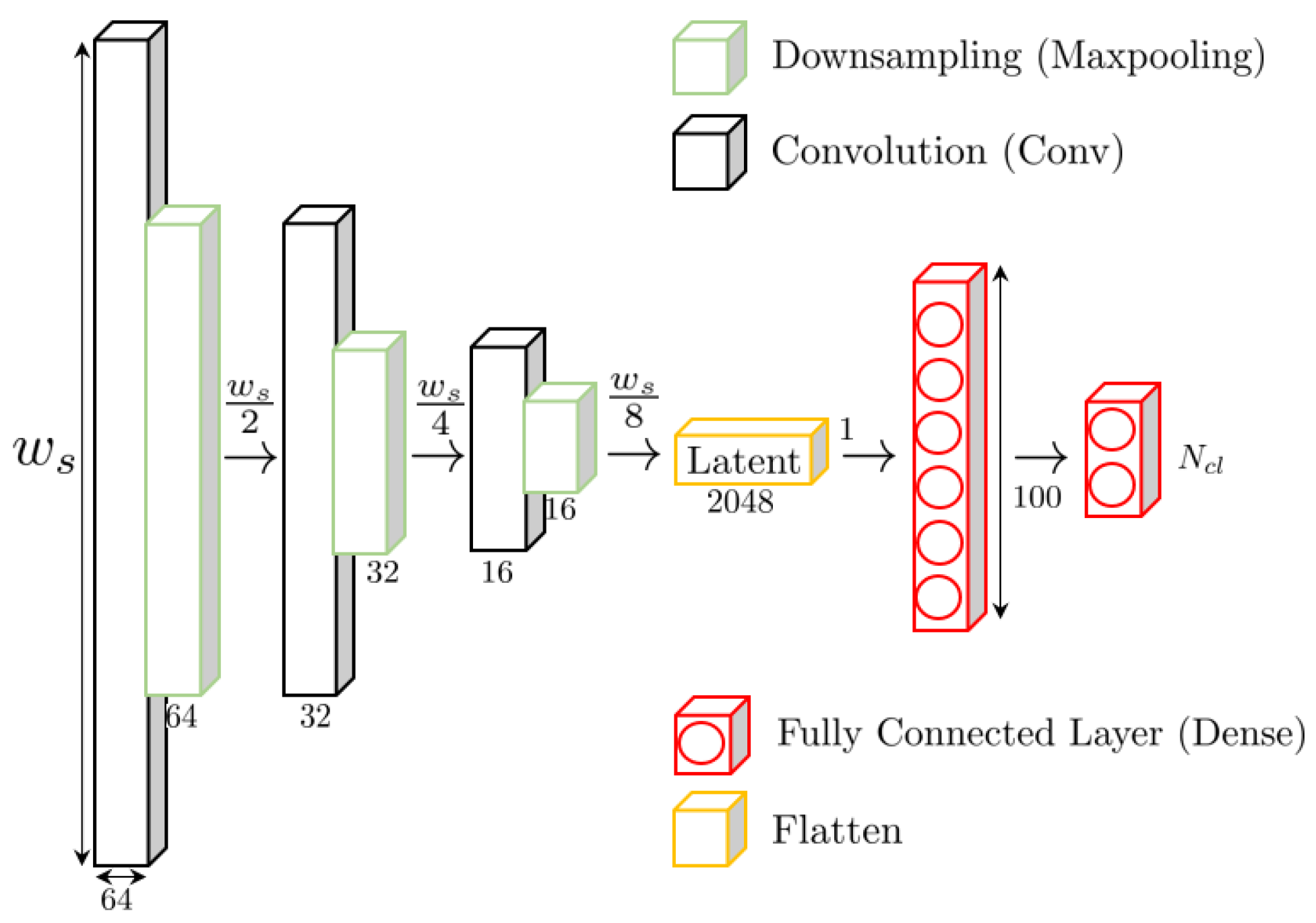
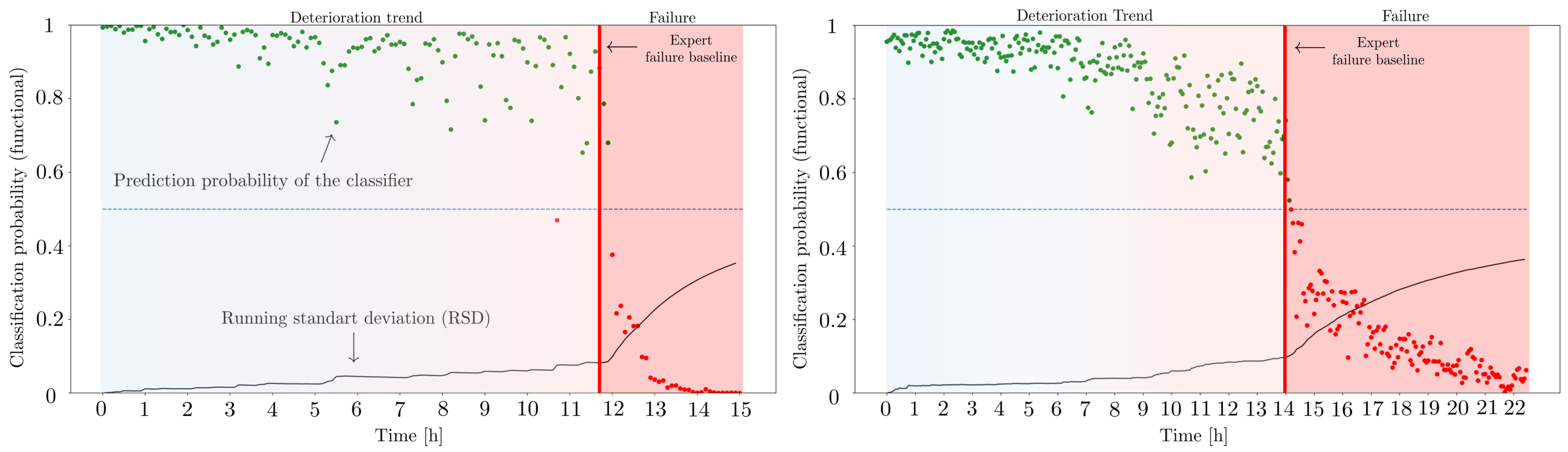
In this part of our research, we delve into the outcomes of our model, operating under the assumption that the quality of the weakly labeled data equals that of a human expert. The trained model, illustrated in Figure 6, proceeds to classify the current health status of the bearing into two categories: ‘functional’ and ‘faulty’. Subsequently, we evaluate the classification probability of the functional class over time, yielding our proposed health index (HI) curve for our device. The results of this approach, as applied to both bearing 1 and bearing 2, are presented in Figure 13.

The HI curves produced by our self-supervised method exhibit the desired coherent trend behavior in both of our bearing test-to-failure experiments. The model predicts both bearings to be in a healthy condition initially and faulty, mirroring the expert ground truth, after 12 h of run-time. To produce this ground truth, the expert reviewed the data by conducting an envelope spectrum analysis, a standard method for bearing evaluation. To us, this comparison to a human baseline seems conclusive since human evaluation is still one of the most common practices in the industry. In comparison to the results of the unsupervised learning methods depicted in Figure 10, the model does not suffer from transient run-in-related effects due to our self-supervised setting. In addition, the model appears to experience increasing uncertainty over time, as reflected in the classification probability beginning to progressively fluctuate. To quantify this loss of conviction, we calculate the running standard deviation (RSD) of the network decision probabilities for the available M test-to-failure measurements in the dataset over time:

$${\sigma }_m=\sqrt{\frac{1}{m-1}\sum _{d=0}^m(y_d-\underset{\mathrm{running}\mathrm{mean}}{\underbrace{\frac{1}{m}\sum _{a=0}^m{y}_a}}){}^2}.$$

(4)

hence for a given time instant $m\in \{0,1,\dots ,M\}$ all classification probability outputs $y_d$ of the network are considered for the calculation of the running standard deviation. The RSD steadily increases over time, indicating a continuous reduction in the model’s confidence that the provided measurements belong to the ‘functional’ class. This observation suggests that our model can successfully capture gradual wear-induced changes in the device prior to the initial fault reported by a human expert envelope spectrum analysis. This capability was not achievable with previous unsupervised methods. Nevertheless, similar to unsupervised approaches, the RSD curve yields an increased slope after approximately 12 h of run-time, which corresponds to the time the initial fault was determined by the human expert.The initial fault is indicated by the red horizontal line in Figure 13.

Similar to the classification probability evaluation, the RSD curves of the self-supervised classifier produced coherent trends for both of our test-to-failure runs. Hence, it might be reasonable to study the use of this model uncertainty measure in terms of self-supervised HI-based RUL prediction in future work.

5.2.2. Impact of Non-Ideal Initial Fault Detection

In the preceding analysis, we operated under the assumption that the quality of the weakly labeled data equaled that of a human expert. However, in real-world scenarios, our unsupervised initial fault detection may not produce labeling results closely aligned with human evaluations. Furthermore, subjective human judgment can lead to slightly different baselines. Hence, it is important to investigate the impact of varying the initial fault times on classifier performance.

To examine this effect, we manually adjusted the labeling threshold for the data, shifting it by up to 15 measurements in either direction around the expert-based decision at shift 0. Subsequently, we employed each newly labeled dataset to train the classifier, following a procedure similar to the previous experiment. Additionally, for each shift, we repeated the training 20 times with different initialization seeds. Considering that our data are recorded at intervals of 10 min (for bearing 1) or 5 min (for bearing 2), the results encompass a time range of 150 to 300 min around the initial fault point determined by the expert, respectively. The results presented in Figure 14 suggest that the classifier’s performance reaches its peak for positive shifts in comparison to the human expert baseline (shift 0). This indicates the positive effect of a later initial fault choice in improving the quality of weak labels. Consequently, the labels provided by the human expert can be considered as a rather conservative estimation of failure.

However, it is noteworthy that all examined shift values yield average classification results exceeding 97% (bearing 1) and 93% (bearing 2). Hence, a slightly earlier or delayed initial fault timing appears to have minimal impact on the self-supervised classifier’s performance.

5.3. Implications, Limitations, and Outlook

In our previous investigations above, we demonstrated several important findings: Firstly, self-supervised learning is capable of generating coherent health index (HI) trends. Secondly, CNN-autoencoders surpass LSTM-autoencoders in creating the weakly labeled data necessary for this process. Finally, we showed that the self-supervised HI can detect wear in the device earlier than human expert analysis and examined how imperfect labeling affects the performance of the self-supervised HI in a bearing test-to-failure scenario. In our study, a shift of up to 300 min had only a minimal effect on the model performance.

Our method, as currently understood, has the potential for application in a variety of scenarios where devices undergo gradual wear, not just in mechanical transmissions. This opens up possibilities for more precise wear monitoring and Remaining Useful Life (RUL) prediction in numerous predictive maintenance situations. However, our testing to date has been limited to a bearing test-to-failure scenario within a controlled environment. The effects of sudden environmental changes on the algorithm’s performance, such as noise interference from nearby machines in sound-based sensor systems, are yet to be explored. Furthermore, the influence of different operational conditions, like varying rotational speeds, on the method’s effectiveness remains to be determined. Consequently, there is a need for further research to extend our findings to different types of bearings, sizes, and devices, enabling the practical application of our method.

6. Conclusions

In this study, we evaluated a novel self-supervised approach to obtain health index (HI) curves for bearing measurements to overcome the challenge of scaling mismatch between curves from different devices. To achieve that, we explored an unsupervised initial fault-based approach to generate weak labels and train a classifier for predicting bearing health over time. Our research shows a notable advancement over previous unsupervised methods: self-supervised approaches yield coherent health index (HI) curves that accurately track the device’s health over time, detecting gradual wear on the bearing earlier than human experts. Additionally, we observed that a CNN autoencoder-based self-supervised learning outperforms the LSTM-based approach. Importantly, our findings indicate that the presence of imperfect weak labels only marginally affects the performance of our proposed self-supervised HI framework.

References

1. Jardine, A.K.; Lin, D.; Banjevic, D. A review on machinery diagnostics and prognostics implementing condition-based maintenance. Mech. Syst. Signal Process. 2006, 20, 1483–1510. [Google Scholar] [CrossRef]
2. Randall, R.B. Vibration-Based Condition Monitoring: Industrial, Automotive and Aerospace Applications; John Wiley & Sons: Hoboken, NJ, USA, 2021. [Google Scholar]
3. Randall, R.B.; Antoni, J. Rolling element bearing diagnostics—A tutorial. Mech. Syst. Signal Process. 2011, 25, 485–520. [Google Scholar] [CrossRef]
4. Jin, X.; Que, Z.; Sun, Y. Development of Vibration-Based Health Indexes for Bearing Remaining Useful Life Prediction. In Proceedings of the 2019 Prognostics and System Health Management Conference (PHM-Qingdao), Qingdao, China, 25–27 October 2019; pp. 1–6. [Google Scholar] [CrossRef]
5. Mosallam, A.; Medjaher, K.; Zerhouni, N. Data-driven prognostic method based on Bayesian approaches for direct remaining useful life prediction. J. Intell. Manuf. 2016, 27, 1037–1048. [Google Scholar] [CrossRef]
6. Gao, R.; Wang, C.; Yan, R.; Malhi, A. A Neural Network Approach to Bearing Health Assessment. In Proceedings of the 2006 IEEE International Joint Conference on Neural Network Proceedings, Vancouver, BC, Canada, 16–21 July 2006; pp. 899–906. [Google Scholar] [CrossRef]
7. Ince, T.; Kiranyaz, S.; Eren, L.; Askar, M.; Gabbouj, M. Real-Time Motor Fault Detection by 1-D Convolutional Neural Networks. IEEE Trans. Ind. Electron. 2016, 63, 7067–7075. [Google Scholar] [CrossRef]
8. Nishat Toma, R.; Kim, J.M. Bearing Fault Classification of Induction Motors Using Discrete Wavelet Transform and Ensemble Machine Learning Algorithms. Appl. Sci. 2020, 10, 5251. [Google Scholar] [CrossRef]
9. Zhao, M.; Zhong, S.; Fu, X.; Tang, B.; Pecht, M. Deep Residual Shrinkage Networks for Fault Diagnosis. IEEE Trans. Ind. Inform. 2020, 16, 4681–4690. [Google Scholar] [CrossRef]
10. Hashemian, H.M. State-of-the-Art Predictive Maintenance Techniques. IEEE Trans. Instrum. Meas. 2011, 60, 226–236. [Google Scholar] [CrossRef]
11. Heimes, F.O. Recurrent neural networks for remaining useful life estimation. In Proceedings of the 2008 International Conference on Prognostics and Health Management, Denver, CO, USA, 6–9 October 2008; pp. 1–6. [Google Scholar] [CrossRef]
12. Malhotra, P.; Tv, V.; Ramakrishnan, A.; Anand, G.; Vig, L.; Agarwal, P.; Shroff, G. Multi-Sensor Prognostics using an Unsupervised Health Index based on LSTM Encoder-Decoder. arXiv 2016, arXiv:cs.LG/1608.06154. [Google Scholar]
13. Vaswani, A.; Shazeer, N.; Parmar, N.; Uszkoreit, J.; Jones, L.; Gomez, A.N.; Kaiser, L.; Polosukhin, I. Attention Is All You Need. arXiv 2023, arXiv:cs.CL/1706.03762. [Google Scholar]
14. Malhotra, P.; Vig, L.; Shroff, G.; Agarwal, P. Long Short Term Memory Networks for Anomaly Detection in Time Series. In Proceedings of the European Symposium on Artificial Neural Networks, ESANN, Bruges, Belgium, 22–24 April 2015. [Google Scholar]
15. Chow, J.; Su, Z.; Wu, J.; Tan, P.; Mao, X.; Wang, Y. Anomaly detection of defects on concrete structures with the convolutional autoencoder. Adv. Eng. Inform. 2020, 45, 101105. [Google Scholar] [CrossRef]
16. Gugulothu, N.; Tv, V.; Malhotra, P.; Vig, L.; Agarwal, P.; Shroff, G. Predicting Remaining Useful Life using Time Series Embeddings based on Recurrent Neural Networks. In Proceedings of the ACM SIGKDD Workshop on Machine Learning for Prognostics and Health Management, San Francisco, CA, USA, 13–17 August 2017. [Google Scholar]
17. Wang, T.; Yu, J.; Siegel, D.; Lee, J. A similarity-based prognostics approach for Remaining Useful Life estimation of engineered systems. In Proceedings of the 2008 International Conference on Prognostics and Health Management, Denver, CO, USA, 6–9 October 2008; pp. 1–6. [Google Scholar] [CrossRef]
18. Wang, T. Trajectory Similarity Based Prediction for Remaining Useful Life Estimation. In ProQuest Dissertations and Theses; University of Cincinnati: Cincinnati, OH, USA, 2010; p. 141. [Google Scholar]
19. Qiu, H.; Lee, J.; Lin, J.; Yu, G. Robust performance degradation assessment methods for enhanced rolling element bearing prognostics. Adv. Eng. Inform. 2003, 17, 127–140. [Google Scholar] [CrossRef]
20. Shin, S.; Lee, S.; Yun, I.; Kim, S.; Lee, K. Joint weakly and semi-supervised deep learning for localization and classification of masses in breast ultrasound images. IEEE Trans. Med. Imaging 2019, 38, 762–774. [Google Scholar] [CrossRef] [PubMed]
21. Jenni, S.; Favaro, P. Self-Supervised Feature Learning by Learning to Spot Artifacts. arXiv 2018, arXiv:1806.05024. [Google Scholar]
22. Senanayaka, J.S.L.; Van Khang, H.; Robbersmyr, K.G. Toward Self-Supervised Feature Learning for Online Diagnosis of Multiple Faults in Electric Powertrains. IEEE Trans. Ind. Inform. 2021, 17, 3772–3781. [Google Scholar] [CrossRef]
23. Wang, D.; Shang, Y. A new active labeling method for deep learning. In Proceedings of the 2014 International Joint Conference on Neural Networks (IJCNN), Beijing, China, 6–11 July 2014; pp. 112–119. [Google Scholar] [CrossRef]
24. Park, S.; Ahn, G.J.; Im, D.H. Auto Labeling Methods Developed Through Semi-Weakly Supervised Learning in Prognostics and Health Management Applications for Rolling Ball Bearing. IEEE Sens. J. 2022, 22, 16223–16233. [Google Scholar] [CrossRef]
25. Truong, C.; Oudre, L.; Vayatis, N. Selective review of offline change point detection methods. Signal Process. 2020, 167, 107299. [Google Scholar] [CrossRef]
26. Malhotra, P.; Ramakrishnan, A.; Anand, G.; Vig, L.; Agarwal, P.; Shroff, G. LSTM-based encoder-decoder for multi-sensor anomaly detection. In Proceedings of the ICML 2016 Anomaly Detection Workshop, New York, NY, USA, 24 June 2016. [Google Scholar]
27. Malhotra, P.; Tv, V.; Vig, L.; Agarwal, P.; Shroff, G. TimeNet: Pre-trained deep recurrent neural network for time series classification. In Proceedings of the 25th European Symposium on Artificial Neural Networks, Computational Intelligence and Machine Learning, Bruges, Belgium, 26–28 April 2017. [Google Scholar]
28. van der Maaten, L.; Hinton, G. Visualizing Data using t-SNE. J. Mach. Learn. Res. 2008, 9, 2579–2605. [Google Scholar]
29. Dunteman, G.H. Principal Components Analysis; Sage: Newcastle upon Tyne, UK, 1989; Volume 69. [Google Scholar]
Figure 1. Schematic of the traditional unsupervised HI generation workflow in the literature.
Electronics 12 04941 g001
Figure 2. Illustration of the HI scaling mismatch induced by unsupervised learning (left) and conventional RUL estimation methods based on curve fitting (middle). The introduction of a time shift in the estimation of RUL is intended to reflect the initial wear of the device caused by manufacturing tolerances. However, the true initial asset condition is unknown. In addition, a schematic of our proposed time-shift independent HI is shown (right).
Electronics 12 04941 g002
Figure 3. Overview of the three steps in our proposed self-self supervised HI curve workflow.
Electronics 12 04941 g003
Figure 4. An illustration of the topology of our studied CNN autoencoder. In the encoder, the given input training sample of size w s is narrowed by a factor of two between layers using max-pooling. The process is repeated until a compression factor c s is achieved. The bottleneck vector is called the latent. An opposing decoder network is trained simultaneously to unravel the encoder compression in order to reconstruct the input.
Electronics 12 04941 g004
Figure 5. Schematic of the wear-induced deterioration trend monitored by the autoencoder reconstruction error over time. The initial fault is used to weakly label the unlabeled measurement data.
Electronics 12 04941 g005
Figure 6. Simple 1D-CNN and fully connected (MLP) layer-based classifier architecture used to estimate the HI based on the weakly labeled data. Note that other supervised architectures are adoptable.
Electronics 12 04941 g006
Figure 7. Sensor positions (left) and test rig structure (right) in our test-to-failure bearing monitoring scenario: (1) motor clutch, (2) back gear, (3) load clutch, (4) coupling gear, (5) tested bearing.
Electronics 12 04941 g007
Figure 8. Illustration on the evaluation of different weak labeling architectures based on their AUC. The required ROC is determined by continuously selecting thresholds in the deterioration curve (left) and calculating its TPR/FPR with respect to an expert ground truth (right).
Electronics 12 04941 g008
Figure 9. Examples of normalized input signals and their corresponding reconstructed signal of the 1D-CNN autoencoders for a damaged and an undamaged bearing measurement.
Electronics 12 04941 g009
Figure 10. Initial fault estimation comparison of our 1D-CNN autoencoder (left) for w s = 128 , c s = 50 % and the LSTM model (right) from Malhotra et al. [26], for bearing 1 from our dataset.
Electronics 12 04941 g010
Figure 11. AUC analysis for the deterioration curve of the CNN (left) and LSTM (right) based autoencoder from Figure 10.
Electronics 12 04941 g011
Figure 12. Latent space visualization based on PCA (top) t-SNE (bottom) for the lifecycle of bearing 1.
Electronics 12 04941 g012
Figure 13. The proposed self-supervised device HI curve depicted for bearing 1 (left) and bearing 2 (right). The provided RSD curve represents the model’s uncertainty that the provided measurement belongs to the ‘functional’ class.
Electronics 12 04941 g013
Figure 14. Overall accuracy of the HI classifier for bearing 1 (left) and bearing 2 (right) as the initial fault detection timing is shifted. Each individual shift corresponds to a delayed (negative shift) or early (positive shift) initial fault estimation compared to the expert initial fault decision at shift zero.
Electronics 12 04941 g014