Article

Accurate Fault Location Method Based on Time-Domain Information Estimation for Medium-Voltage Distribution Network

1
Electric Power Research Institute of State Grid Hubei Electric Power Company, Wuhan 430070, China
2
State Key Laboratory of Alternate Electrical Power System with Renewable Energy Sources, North China Electric Power University, Baoding 071003, China
*
Author to whom correspondence should be addressed.
Electronics 2023, 12(23), 4733; https://doi.org/10.3390/electronics12234733
Submission received: 20 October 2023 / Revised: 17 November 2023 / Accepted: 20 November 2023 / Published: 22 November 2023

Abstract

:
The sampling rate of the wide-area synchronous phasor measuring device (D-PMU) in the distribution network is insufficient, and the localization sensitivity of the traditional localization method based on the time-domain Bergeron equation in the distribution network is insufficient. In this paper, an accurate location method of the distribution line grounding fault based on the time-domain’ synchronous information calculation is proposed to solve the problem of limited location accuracy caused by a low sampling rate and the insufficient sensitivity of traditional methods. The method preprocesses the measurement data through low-frequency time-domain signal reconstruction and cubic spline interpolation. The fault current’s different location criterion is constructed by using the voltage and current constraints at the fault point. By calculating the fault current difference at a limited number of calculated points, the accurate fault location under a low sampling rate is realized, which is beneficial to the rapid maintenance of faults and the shortening of the power outage time.

1. Introduction

Medium-voltage distribution network (MVDN) faults occur frequently, accounting for about 75% of power outages, and most of them are ground faults [1]. The transition resistance of a grounding fault is high, and the evolution process is complex and is closely related to the neutral grounding mode, which usually presents the characteristics of weak and intermittent signals [2]. The accurate fault location of MVDN is the main method to speed up the line repair, reduce the power outage time, and quickly restore the power supply. It is also the key technology to further improve the automation level and power supply reliability of MVDN [3].
In recent years, D-PMU devices and systems have been gradually recognized and applied in the MVDN, which provides solid support for the use of transient quantities to solve the problem of fault detection and location in the MVDN [4]. The accurate fault location technology of MVDN mainly includes section location and fault location [5]. Fast section location helps to quickly isolate fault areas and restore the power supply in non-fault areas. Accurate fault location is conducive to the timely repair of lines and shortening the power outage time.
At present, distribution network fault location methods are mainly divided into the traveling wave method, impedance method, and artificial intelligence method. The traveling wave positioning method mainly includes the cell-type traveling wave location method and network-type traveling wave location method. Due to the complex structure of distribution networks, it is very difficult to identify the reflected traveling wave at fault points. The double-ended traveling wave method has high requirements for time synchronization, so it is difficult to accurately calculate the fault distance under the condition of large time synchronization errors. Network traveling wave fault location can accurately locate faults even when the measuring device fails, and has a certain tolerance of the traveling wave arrival time error. However, when the network contains a ring network structure, there are multiple traveling wave transmission paths between the measuring points. If the traveling wave transmission paths cannot be correctly matched, the network traveling wave location will fail.
The impedance method mainly uses time-domain measurement information for fault location [6]. The accurate fault location method of MVDN based on the time-domain transient component is mainly derived and summarized using fault analysis. Then, according to the location principle, a location equation that directly contains the fault distance parameter or can indirectly reflect the fault distance information is constructed [7]. The appropriate mathematical method is selected to solve the equation and locate the fault location [8]. In Reference [9], the fault distance is calculated iteratively by using the measured data at both ends of the line according to the constraint that the voltage at the fault point remains unchanged. Due to the complex network structure and variable operation mode of medium-voltage distribution networks, the above method is difficult to be applied in practical engineering. To accelerate the convergence of iteration, the distribution characteristics of the line voltage amplitude are studied in [10], and the line is divided into regions according to its monotonicity. The tangent intersection theory is used to calculate the fault distance in the region and the location accuracy is corrected by iteration. Reference [11] proposed a location principle based on the minimum variance of the transition resistance at the fault point to achieve an accurate fault location. The positioning accuracy of this method depends on the identification accuracy of the transition resistance and the fault location accuracy is still affected by the operating mode of the system. The methods mentioned in references [9,10,11] can be classified as the two-end method, which is designed based on the measurement data at both ends of the line. They have high requirements for data synchronization, which is difficult for traditional measuring devices to meet the requirements of data synchronization [12,13,14].
The single-ended methods only use the measurement information at one end of the line. They can regard the fault distance as an unknown parameter, and overcome the location error caused by time synchronization through parameter identification [15]. In reference [16], for the single-phase grounding fault, the mode voltage of the fault point and the mode current flowing into the fault point at the local end are calculated by using the transient voltage and current data at the local end. Then, the voltage and current at the opposite end are estimated by using the mode voltage at the fault port. On this basis, the mode current flowing into the fault point at the opposite end is calculated, and the location equation is constructed based on the basic principle that the time of the 0-mode, 1-mode, and 2-mode current at the fault point is equal. Reference [17] proposed a time-domain single-ended location method based on the Mayr arc model. By analyzing the fault characteristics of the arc, the similarity criterion of the waveform is constructed by using the characteristics of the time-domain waveform of the arc at the fault point as a square wave. At the same time, according to the location accuracy requirements, the virtual observation points are set along the fault line, and the fault location is realized by comparing the waveform similarity of the virtual observation points. However, the fault location accuracy of this method is easily affected by the calculation error of the voltage and current. When the impedance method is used to locate faults in the frequency domain, it is difficult to accurately extract power frequency components because of the weak single-phase grounding fault signal of a non-effective grounding distribution network. Therefore, the traditional impedance method is mostly used to locate faults between phases. The single-ended time-domain location method is greatly affected by the transition resistance. In view of this difficulty, reference [18] calculates the transition resistance through the active power to compensate for the measured impedance. Reference [19] studied the arc dynamic model based on the Thomson principle to reflect the change of the arc resistance. However, the above-mentioned single-ended time-domain location method is based on the same phase between the measured current and the fault point current, and there are principle defects. In addition, the single-ended time-domain location method has poor adaptability to the MVDN structure with multiple T-connected branches, and the location accuracy is not high.
As for the artificial intelligence methods, the fault location is realized by solving the model through an artificial intelligence algorithm. The literature [20] proposes a fault section location method based on a genetic algorithm, which solves multi-solution problems by introducing the concept of a minimum set and improves the fault tolerance of the algorithm. In the literature [21], hierarchical modeling is carried out according to the multi-branch tree structure of the distribution network, which reduces the dimension of the optimization model and effectively improves the solving speed. In addition, the ant colony algorithm [22], harmonic algorithm [23], Bayesian estimation [24], particle swarm algorithm [25], other artificial intelligence algorithms have been applied to the fault section location. Artificial intelligence models can locate the fault section accurately in the case of overcurrent information distortion and a missing alarm. However, the construction is relatively complex. In some special scenarios, incorrect location results may be obtained.
In addition to the above fault location methods, with more and more attention paid to the intelligent construction of MVDN, some theoretical studies [26] and projects have applied PMU to MVDN. Reference [27] proposed a fault location method for multi-power MVDN based on PMU. Using the voltage and current measurement information of PMU, each line segment is iteratively solved to calculate the suspected fault line and its fault distance, and then the actual fault position is obtained by the voltage phase relationship between the fault voltage at both ends of PMU and the measured voltage. Aiming at the characteristics of many feeder branches and generally short lines in the MVDN, based on the distributed parameter model, the voltage and current measurement information of the PMU at the end of the line after the fault occurs is used to calculate the voltage of each branch point and identify the fault branch accordingly [28]. Further, according to the voltage distribution at both ends of the fault branch, the fault distance is calculated. However, the above methods have high requirements for the sampling rate of the measurement and the practical effect needs to be verified. However, using the low-frequency band time-domain signal reconstruction and the pre-processing of the measurement data can improve the actual sampling rate and further improve the fault location accuracy.
This paper studies the accurate location of the distribution line grounding fault based on the time-domain information calculation and proposes a new method of accurate fault location. On the premise that the fault section has been accurately located, aiming at the problem that the measurement sampling rate is insufficient and the traditional time-domain Bergeron positioning method is not sensitive enough in the distribution network, the low-frequency time-domain signal reconstruction and cubic spline interpolation method are proposed to preprocess the data. Then, the fault current difference location criterion is constructed based on the voltage and current constraint conditions at the fault point to achieve an accurate location under a low sampling rate. Finally, the PSCAD/EMTDC simulation verifies the applicability of the method under different working conditions and also considers the influence of the neutral point grounding mode, initial fault phase angle, and transition resistance on the locating results.
In this paper, Section 2 introduces the principle of the time-domain Bergeron location. The location method based on the time-domain information estimation is proposed in Section 3. Simulation results are presented in Section 4. And Section 5 gives the conclusion.

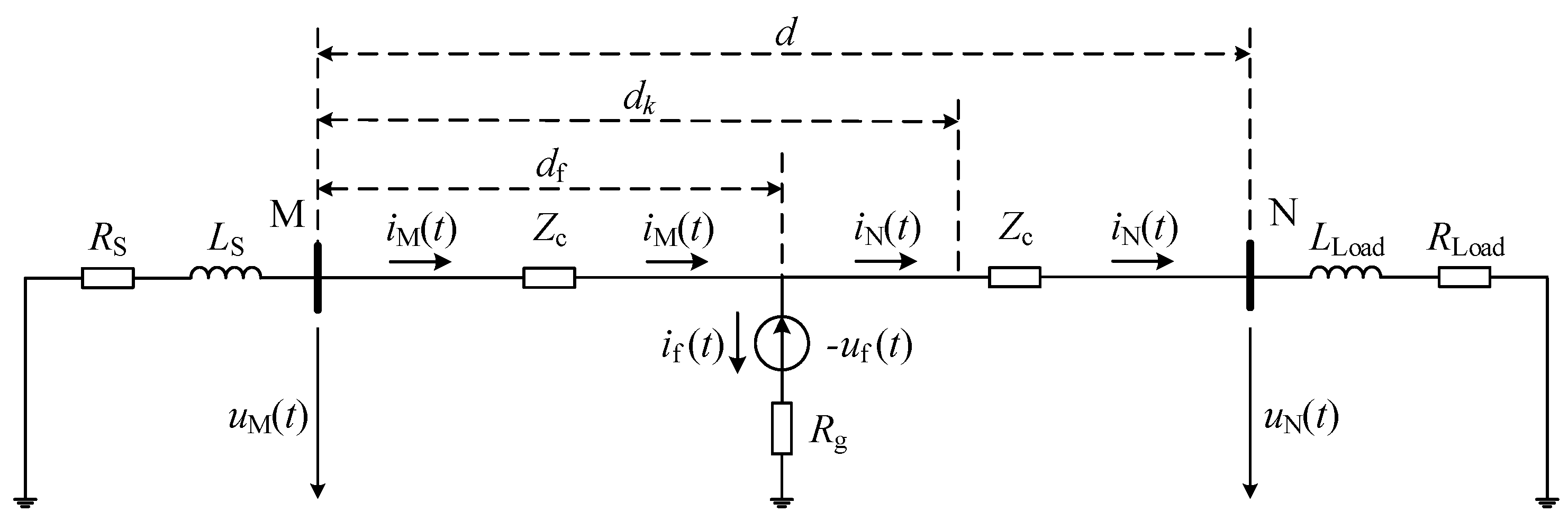
2. Time-Domain Bergeron Location Principle

2.1. Basic Location Principle

For the single-phase system, the time-domain Bergeron recursive formula based on the distributed parameter model is Equation (1). When the voltage and current at a certain point of the line are known, the voltage and current distribution along the line can be calculated.
{ u x ( x , t ) = 1 2 [ u ( t + τ ) Z c i ( t + τ ) ] + 1 2 [ u ( t τ ) + Z c i ( t τ ) ] i x ( x , t ) = 1 2 Z c [ u ( t + τ ) Z c i ( t + τ ) ] 1 2 Z c [ u ( t τ ) + Z c i ( t τ ) ]
where u x ( x , t ) and i x ( x , t ) are the voltage and current values along the line, u ( t ) and i ( t ) are the actual measured voltage and current at a certain point, τ is the transmission time, τ = x / v , x is the calculated distance, v is the wave velocity, Z c is the wave impedance, and Z c = L / C .
Figure 1 shows the equivalent circuit diagram of the faulty component network of the single-phase system. In the diagram, u M ( t ) and u N ( t ) are the voltage at both ends of the fault line, i M ( t ) and i N ( t ) are the current at both ends of the fault line, Z c is the wave impedance of the distributed parameter line model, R S and L S are the equivalent resistance and inductance of the system represented by lumped parameters, R Load and L Load are the equivalent resistance and inductance of the load represented by lumped parameters, u f ( t ) is the additional voltage source voltage at the fault point, i f ( t ) is the current at the fault point, R g is the grounding resistance at the fault point, d is the length of the fault line, d f is the distance from the fault point to the M point in the fault line, and d k is the distance from a point (k) to the M point in the fault line.
According to the time-domain Bergeron recursive formula and the direction of the voltage and current, shown in Figure 1, Equations (2) and (3) can be written, that is, the voltage and current at the fault point can be calculated, by using the measured data at both ends of the section.
The M-end measurement data are expressed as:
{ u fM ( d f , t ) = 1 2 [ u M ( t + d f v ) Z c i M ( t + d f v ) ] + 1 2 [ u M ( t d f v ) + Z c i M ( t d f v ) ] i fM ( d f , t ) = 1 2 Z c [ u M ( t + d f v ) Z c i M ( t + d f v ) ] + 1 2 Z c [ u M ( t d f v ) + Z c i M ( t d f v ) ]
The N-end measurement data are expressed as:
{ u fN ( d d f , t ) = 1 2 [ u N ( t + d d f v ) + Z c i N ( t + d d f v ) ] + 1 2 [ u N ( t d d f v ) Z c i N ( t d d f v ) ] i fN ( d d f , t ) = 1 2 Z c [ u N ( t + d d f v ) + Z c i N ( t + d d f v ) ] 1 2 Z c [ u N ( t d d f v ) Z c i N ( t d d f v ) ]
where u f ( d f , t ) is the M-end voltage of the fault point, u f ( d d f , t ) is the N-end voltage of the fault point, i fM ( d f , t ) is the M-end current of the fault point, and i fN ( d d f , t ) is the N-end current of the fault point.
At the fault point ( d k = d f ) , the additional voltage source voltage calculated from the voltage and current of M and N can be expressed as Equation (4). That is, without considering the line parameters and measurement and calculation errors, the voltage values calculated from the measurement data at both ends of the fault line are always equal at the fault point.
u f ( t ) = u fM ( d f , t ) = u fN ( d d f , t )
At the non-fault point ( d k d f ) , the voltage calculated from the voltage and current of M and N is not equal, and Equation (5) can be obtained. The farther the d k is from d f , the greater the difference between u M ( d k , t ) and u N ( d d k , t ) is.
u M k ( d k , t ) u N k ( d d k , t )
According to Equations (4) and (5), the fault location criterion shown in Equation (6) can be constructed, which is also the general criterion of the fault location method based on the Bergeron equation in the time domain.
Δ u f ( t ) = | u fM ( d f , t ) u fN ( d d f , t ) | = 0
The above location principle is based on the analysis of a single-phase system. For the three-phase system, due to the existence of phase-to-phase coupling, the three-phase measurement data need to be preprocessed before calculating the fault location. Using the appropriate phase–mode transformation matrix, the three-phase coupling network is decomposed into independent 1-, 2-, and 0-mode networks. At the same time, the line parameters also need to be converted into corresponding modulus data, and then the fault location is realized according to the location criterion. For ground faults, the 0-mode component has more obvious fault characteristics than the line-mode component (1-mode or 2-mode). Therefore, the 0-mode current component is usually used for accurate fault location.

2.2. Influencing Factors of Location Accuracy

It can be seen from Equation (1) that when the time-domain Bergeron equation is used to calculate the voltage and current along the line, the data accuracy mainly depends on the measurement accuracy of the measured data and the calculation accuracy of the transmission time τ . In this paper, D-PMU is used as the signal acquisition device, and the synchronous measurement data collected by it are accurate and reliable by default. Therefore, only the influence of the calculation accuracy of the transmission time τ is analyzed.
Considering that the collected measurement data are discrete data, Equation (1) is discretized, that is:
{ u x ( x , t ) = 1 2 [ u ( t + s f s ) Z c i ( t + s f s ) ] + 1 2 [ u ( t s f s ) + Z c i ( t s f s ) ] i x ( x , t ) = 1 2 Z c [ u ( t + s f s ) Z c i ( t + s f s ) ] 1 2 Z c [ u ( t s f s ) + Z c i ( t s f s ) ]
where u x ( x , t ) and i x ( x , t ) are the discretized voltage and current along the line, u ( t ) and i ( t ) are discrete sampling data, f s is the sampling rate, T s = 1 / f s , T s is the sampling interval, s f s is a discrete form of t, and s is a positive integer.
Comparing Equations (1) and (7), the difference between the actual transmission time τ ( τ = x v ) and the calculated transmission time τ * ( τ * = s f s ) is:
Δ τ = x v s f s
When the calculated transmission time τ * is accurate enough, Δ τ = 0 , that is:
x = ν s f s
Let s = 1 , that is, when f s is the sampling rate and the wave velocity is v , there is a minimum calculated distance:
x min . f s = ν f s
When the calculated distance x x min . f s , the calculated voltage and current data are the voltage and current at point x min . f s , so the minimum calculated distance is the fault location accuracy. In addition, since the wave velocity is generally regarded as a constant, the fault location accuracy depends on the sampling rate. The higher the sampling rate, the higher the fault location accuracy. Further, when the preset calculation distance is fixed, the calculation accuracy is affected by the sampling rate. The higher the sampling rate is, the more accurate the calculated τ is, that is, the closer the u x ( x , j ) and i x ( x , j ) calculated by Equation (7) are to the real data, and the more accurate the fault distance calculated by the calculated data is.
Referring to the technical index of D-PMU, the sampling rate is f s 10   kHz . Using the zero-mode wave velocity of the typical distribution lines in the simulation environment, v = 1.8 × 10 8   m / s , the minimum estimated distance is x min .10 kHz = 18   km , which is far from meeting the fault location accuracy requirements of the MVDN. In order to meet the requirements of location accuracy (taking 200 m as an example), the sampling rate should be at least 2 MHz. Therefore, a high sampling rate is a prerequisite for accurate fault location using time-domain Bergeron equation data. However, the sampling rate of MVDN measurement devices is generally low at this stage. Even for advanced measurement devices (such as D-PMU, FTU, etc.), it is difficult for its sampling rate to meet the accuracy requirements of the accurate fault location in MVDNs.
The following analyzes the performance characteristics of zero-mode voltage and zero-mode current when the fault occurs. There are many branch nodes in the MVDN and the lines are generally short. The zero-mode voltage with a linear distribution along the line has little difference in the faulty section, as shown in Figure 2a. Each measuring point (MP) is distributed on both sides of the upstream and downstream of the fault point. At this time, if the location criterion shown in Equation (6) is adopted, the voltage difference calculated along the faulty section may be very small and the fault location sensitivity is low, which can easily cause location failure. The zero-mode current is mainly determined by the line-to-ground capacitance current. The zero-mode currents detected upstream and downstream of the fault point are generally quite different, as shown in Figure 2b. At this time, the fault current difference is used as the location criterion, which is more conducive to accurate fault location.

3. Location Method Based on Time-Domain Information Estimation

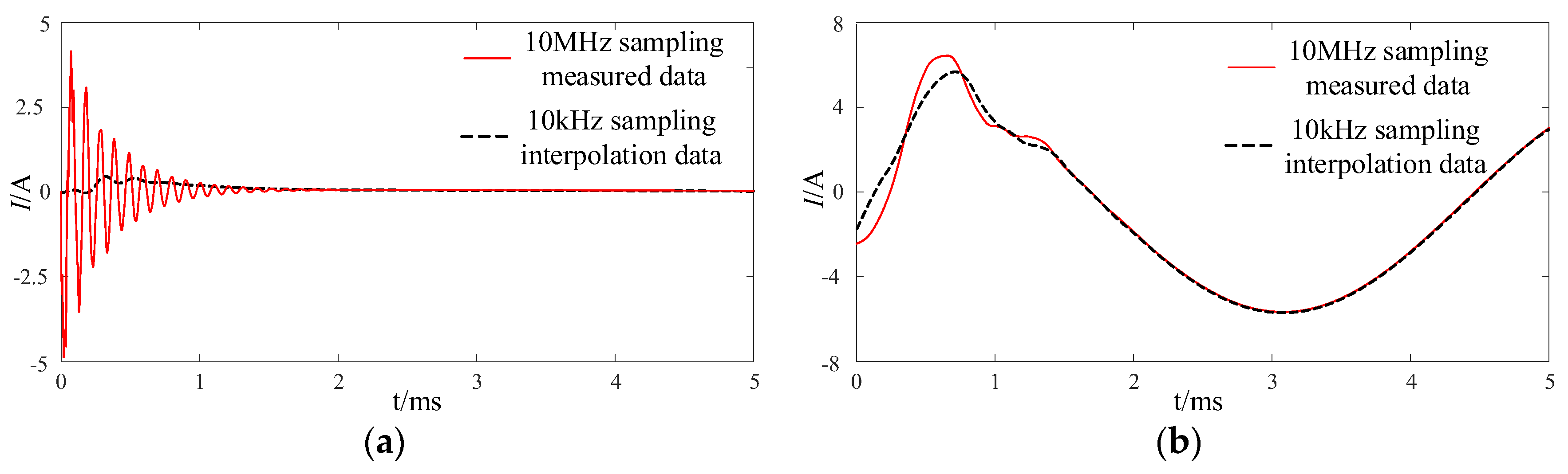
3.1. Data Pre-Processing Method at Low Sampling Rate

When the sampling rate of D-PMU cannot meet the accuracy requirements of MVDN, data preprocessing is used to achieve the accurate fault location of MVDN. The cubic spline interpolation function has good stability, strong convergence, and is less affected by harmonics. The waveform obtained by interpolation is smooth. Using it to calculate the electrical quantity at the non-sampling time, the data satisfying the location requirements can be obtained. Let x ( t ) be a cubic spline interpolation function, x k is the sampling value at the sampling time t k , and the sampling interval is T s . Then, when t [ t k , t k + 1 ] , there is:
x ( t ) = 1 T s 3 { ( t t k + 1 ) 2 [ T s + 2 ( t t k ) ] x k + ( t t k ) 2 [ T s + 2 ( t k + 1 t ) ] x k + 1 }                     + 1 T s 2 { [ ( t t k + 1 ) 2 ( t t k ) ] x k + [ ( t t k ) 2 ( t t k + 1 ) ] x k + 1 }
where x k = ( x k x k 1 ) / 2 T s .
In the fault transient process, the refraction and reflection of the wave and its characteristic evolution are very complex. If cubic spline interpolation is directly performed on the sampled data, the original signal waveform cannot be realistically reflected, which will lead to data distortion. Using wavelet decomposition and reconstruction technology, the full-band signal collected by D-PMU is processed, and the low-frequency band time-domain signal is extracted. On this basis, the voltage and current values at the non-sampling time are calculated by cubic spline interpolation function, so as to ‘improve’ the data sampling rate and obtain more real signal data. Taking the current signal as an example, the sampling rate of the full-band signal and the low-frequency band signal at 10 kHz is ‘raised’, and the effect is shown in Figure 3. In the figure, the interpolation effect based on the full-band signal is not good, and the waveform obtained by interpolation has a great error with the waveform obtained by the actual 10 MHz sampling, which cannot reflect the original signal waveform. Based on the interpolation processing of low-frequency band signals, there is a certain error in waveform fitting at the beginning of the fault. Additionally, 1.5 ms after the fault time, the waveform obtained by interpolation completely coincides with the waveform obtained by the actual 10 MHz sampling, and the data reduction degree is high.
In summary, in order to effectively solve the problem that it is difficult to achieve an accurate fault location due to the insufficient actual sampling rate of D-PMU, data processing can be carried out by cubic spline interpolation and low-frequency band time-domain signal reconstruction technology to obtain data that meet the requirements of location accuracy, and then, accurate fault location can be carried out.

3.2. The Location Principle of Estimating Current Based on Time-Domain Bergeron

At the fault point ( d k = d f ) , Equation (4) always holds, and the combined Equations (2) and (3) can be obtained:
u M ( t d f v ) + u M ( t + d f v ) u N ( t d d f v ) u N ( t + d d f v ) = Z c [ i M ( t + d f v ) i M ( t d f v ) + i N ( t + d d f v ) i N ( t d d f v ) ]
Further:
u M ( t + d f v ) + u M ( t d f v ) u N ( t + d d f v ) + u N ( t d d f v ) = Z c [ i M ( t + d f v ) i M ( t d f v ) + i N ( t + d d f v ) i N ( t d d f v ) ] + 2 [ u M ( t + d f v ) u N ( t d d f v ) ]
According to Figure 1, the fault current at the fault point ( d k = d f ) can be calculated by Equation (14).
i f ( t ) = i Mf ( d f , t ) i Nf ( d d f , t )
By sorting out Equations (2), (3), and (14), we can get:
i f ( t ) = 1 2 Z c { [ u M ( t + d f v ) + u M ( t d f v ) u N ( t + d d f v ) + u N ( t d d f v ) ]         + Z c [ i M ( t + d f v ) + i M ( t d f v ) i N ( t + d d f v ) i N ( t d d f v ) ] }
Substituting Equation (13) into Equation (15), the calculation formula of the reference current at the fault point is obtained:
i f ( t ) = [ 1 Z c u M ( t d f v ) + i M ( t d f v ) ] [ 1 Z c u N ( t + d d f v ) + i N ( t + d d f v ) ]
Similarly, when ignoring the line parameters and measurement and calculation errors, Equation (15) is equivalent to Equation (16) at the fault point ( d k = d f ) .
i f ( t ) = i f ( t )
At the non-fault point ( d k d f ) , because of u M k ( d k , t ) u N k ( d d k , t ) , then:
i f ( t ) i f ( t )
In summary, the fault location can be determined by measuring the data at both ends of the faulty section and recursively calculating the fault current difference Δ i f ( t ) .
Δ i f ( t ) = | i f ( t ) i f ( t ) | = 0

3.3. Location Method Based on Time-Domain Bergeron Current Estimation

To meet the requirements of fault location accuracy and reduce the Bergeron calculation amount in the time domain, the calculation point is set with a calculation step length of less than or equal to half of the length of the fault location accuracy. Only the fault current difference at the calculation point is calculated, and the actual fault location is characterized by the calculation point. Obviously, according to the above method for fault location, the location accuracy can still meet the requirements. It should be noted that it is necessary to use the D-PMU-measured voltage and current data at both ends of the faulty section to calculate the current distribution point by point along the line. At this time, the actual MPs at both ends of the section are also regarded as the calculation points.
k = ceil ( 2 x * x j )
x n = { 0.5 x j                         ( n = 1 , 2 , k 1 ) x * 0.5 ( k 1 ) x j                                     ( n = k )              
where n ( n = 1 , 2 , , k ) is the calculated point, k is the total number of calculated points, x * is the length of the faulty section, and x j is the required length of the fault location accuracy.
Then, the voltage and current of the calculated point n ( n = 1 , 2 , , k ) are calculated using the M-end measurement data:
{ u M . n ( t ) = 1 2 [ u M ( t + n T t ) Z c i M ( t + n T t ) ] + 1 2 [ u M ( t n T t ) + Z c i M ( t n T t ) ] i M . n ( t ) = 1 2 Z c [ u M ( t + n T t ) Z c i M ( t + n T t ) ] + 1 2 Z c [ u M ( t n T t ) + Z c i M ( t n T t ) ]
Comprehensive Equations (1), (7), and (22):
n T t = s f s = n x n v
Similarly, the voltage and current of the calculated point n ( n = 1 , 2 , , k ) are calculated by using the N-end measurement data:
{ u N . n ( t ) = 1 2 { u N [ t + ( k 1 n ) T t ] + Z c i N [ t + ( k 1 n ) T t ] } + 1 2 { u N [ t ( k 1 n ) T t ] Z c i N [ t ( k 1 n ) T t ] } i N . n ( t ) = 1 2 Z c { u N [ t + ( k 1 n ) T t ] + Z c i N [ t + ( k 1 n ) T t ] } 1 2 Z c { u N [ t ( k 1 n ) T t ] Z c i N [ t ( k 1 n ) T t ] }
By combining Equations (22) and (24), Equation (15) can be modified as:
i f . n ( t ) = 1 2 Z c { u M ( t + n T t ) + u M ( t n T t ) u N [ t + ( k 1 n ) T t ] + u N [ t ( k 1 n ) T t ] } +   1 2   { i M ( t + n T t ) + i M ( t n T t ) i N [ t + ( k 1 n ) T t ] i N [ t ( k 1 n ) T t ] }
Similarly, Equation (15) can be modified as:
i f . n ( t ) = [ u M ( t + n T t ) Z c i M ( t + n T t ) ] { u N [ t ( k 1 n T t ) ] Z c i N [ t ( k 1 n T t ) ] }
In summary, when the fault current at the estimated point n satisfies Equation (27), it is determined that n is the fault point, and the distance from the point to both ends of the section is the fault distance.
Δ i f . n ( t ) = min | i f . n ( t ) i f . n ( t ) |
On this basis, considering the influence factors such as a measurement error, bad data, and line parameters, the fault location can be determined only by calculating the fault current difference A at a certain sampling time, which may cause misjudgment. Therefore, the multi-time measurement data are comprehensively used for the fault location to improve the accuracy, that is, the criterion is:
min ( j = 1 N | Δ i f . n ( t j ) | )

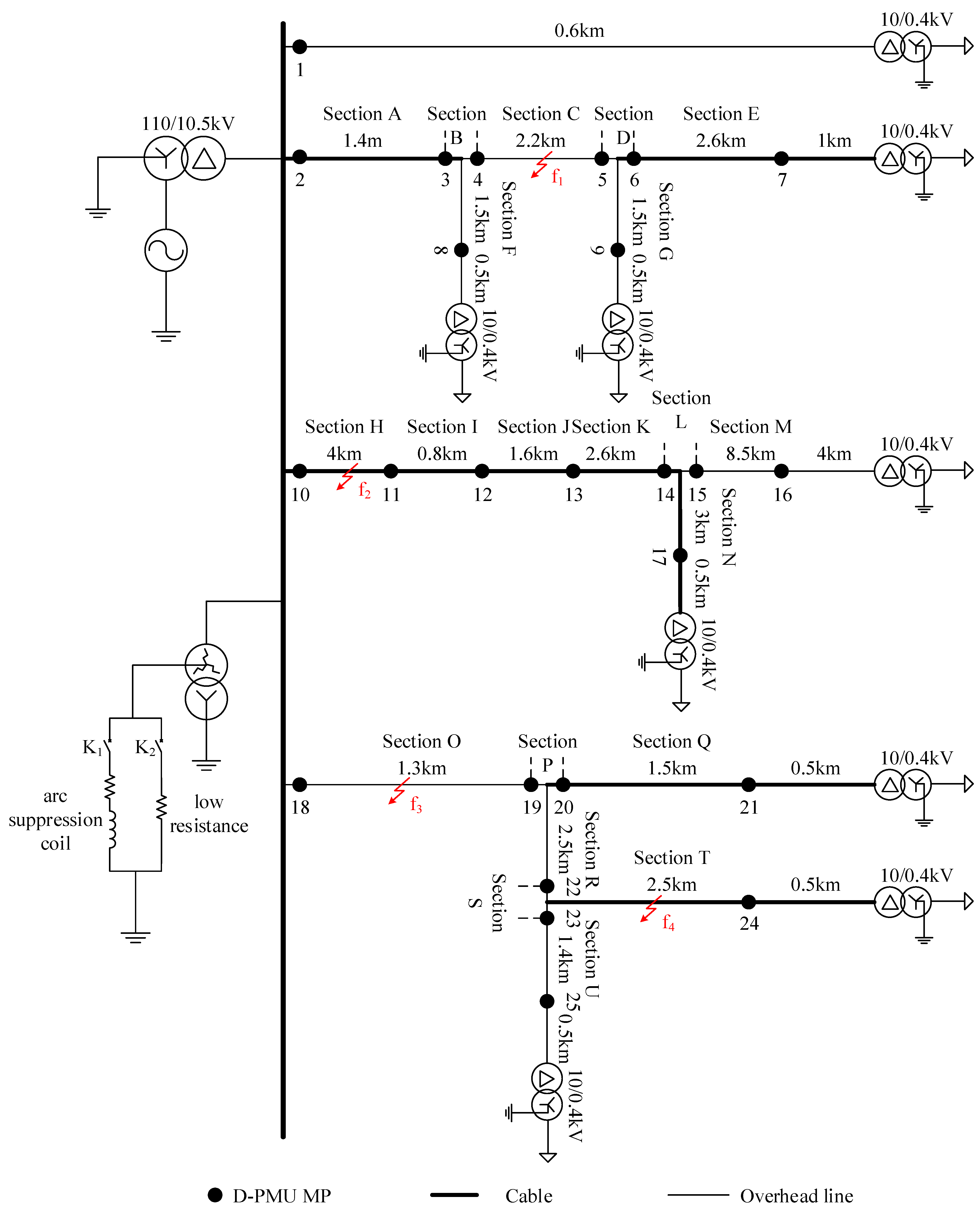
4. Simulation Analysis

The 10 kV MVDN, which is widely used in field engineering, is simplified. Considering the main transformer, grounding transformer, distribution transformer, neutral point grounding device, overhead, cable, and overhead-cable hybrid branch feeder, the MVDN simulation model with multiple T-connected branch lines is established in PSCAD/EMTDC, as shown in Figure 4. The precondition of the proposed method is that the faulty section has been accurately located. The following simulations are based on the location of the faulty section. It is assumed that the sampling rate is 10 kHz, the fault location accuracy is 200 m, and the calculation step is 100 m.

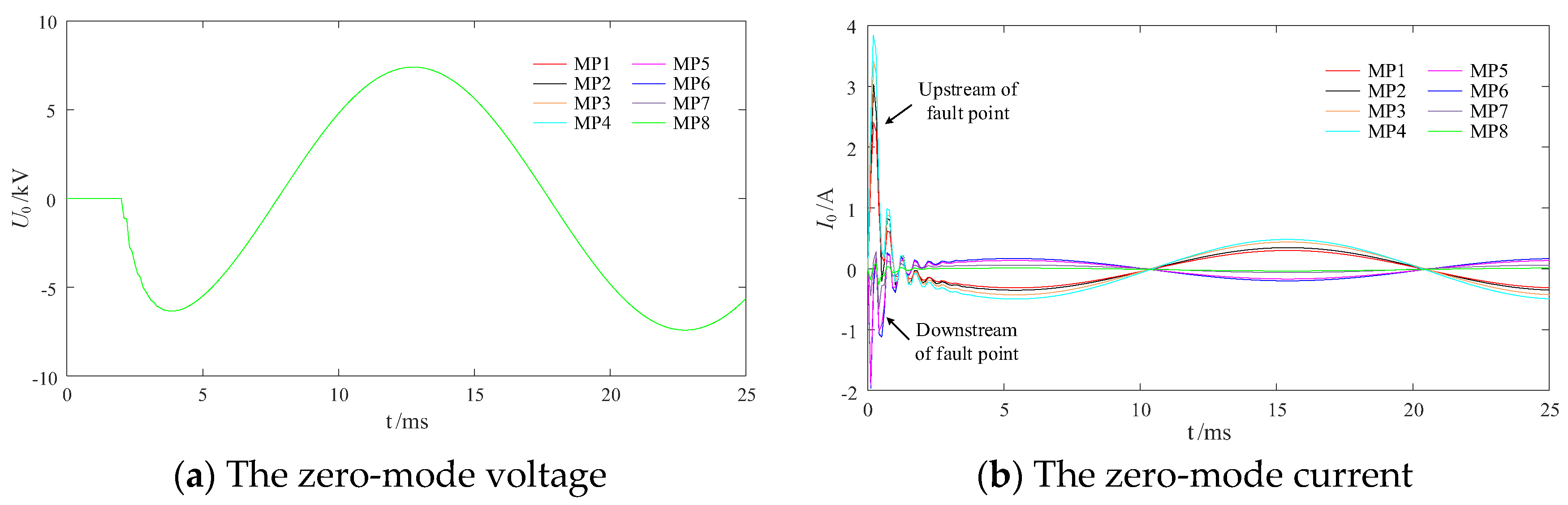
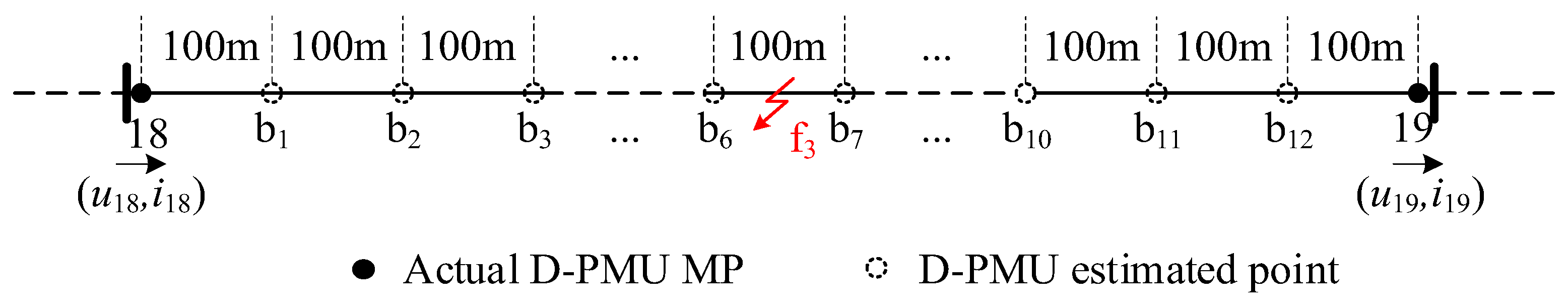
4.1. Example Fault f3 Analysis

The single-phase grounding fault is set at f3, the initial phase angle of the fault is 30°, the transition resistance is 1000 Ω, and the known faulty section is Section O. On this basis, the accurate location method of the grounding fault of the distribution line based on the time-domain information is used to further determine the fault location.
The length of the O line in the known section is 1.3 km, and the calculation points are set according to Equations (20) and (21), as shown in Figure 5. In the Figure, 18 and 19 are the actual D-PMU measuring points and b1~b12 are the calculated points. The measurement data of D-PMU18 and D-PMU19 are processed by cubic spline interpolation and low frequency band time-domain signal reconstruction technology, respectively, and the sampling rate is increased to 10 MHz. Further, the current information at the estimated point is calculated according to Equations (22) and (24), and the fault current difference is calculated by combining Equations (25), (26) and (28). The results are shown in Table 1. It can be seen from the table that the location of the fault is the estimated point b8, that is, the fault is determined to occur at 800 m from the first end of the section. The actual fault location of fault f3 is 650 m away from the first end of section O (MP18). At this time, the location error is | 650 800 | = 1 50   m   200   m , it can meet the requirements of the fault location accuracy.
If the voltage information of each estimated point is still calculated according to Equations (22) and (24), and Equation (6) is used as the fault location criterion, the calculation results are shown in Table 2. The difference in the fault voltage calculated by each calculation point is very small, and the difference of some measurement points is the same or even zero. At this time, the fault location fails. The simulation results are consistent with the calculation of the fault voltage difference described in Figure 2, which will result in low sensitivity of the fault location and the inability to achieve an accurate location. Therefore, this paper adopts the accurate fault location based on the fault current difference.

4.2. Analysis of the Influence of Neutral Grounding Mode

For the three grounding methods commonly used in the MVDN: neutral point ungrounded, arc suppression coil grounded, low-resistance grounded, a fault initial phase angle of 60°, a transition resistance of 1500 Ω, and the location results are shown in Table 3.
It can be seen from Table 3 that the influence of the neutral point grounding mode on the proposed method is negligible. The absolute error of positioning results under any neutral grounding mode is within 200 m, thus the accurate location results of faults are accurate and reliable.

4.3. Analysis of the Influence of Fault Conditions

For different fault initial phase angles and transition resistances, it is assumed that the distribution system adopts the neutral point ungrounded mode. When a single-phase ground fault occurs at f1, f2, f3, and f4, the fault initial phase angle changes from 0° to 90°, and the transition resistance ground fault changes from 0 Ω to 2000 Ω. The fault location results are shown in Table 4. It can be seen from the table that under different fault locations, fault initial phase angles, and transition resistance conditions, although there is a certain error between the fault location results and the actual fault location, the absolute error is less than or equal to 200 m, which meets the requirements of fault location accuracy. Accordingly, it can be concluded that the fault initial phase angle and transition resistance have no effect on the proposed method.

4.4. Sampling Rate Impact Analysis

The sampling rate of the above simulation analysis is 10 kHz. It is necessary to ‘improve’ the data sampling rate by cubic spline interpolation and low-frequency band time-domain signal reconstruction technology to obtain the data that meet the requirements of a precise fault location. With the progress and development of MVDN construction, the sampling rate of PMU will continue to increase in the future, and the measured data can meet the requirements of an accurate fault location. Based on this, according to different actual sampling rates, the location results of single-phase grounding faults at fault locations f1, f2, f3, and f4 are analyzed. It is assumed that the distribution system adopts the neutral point ungrounded mode, the initial phase angle of the fault is 0°, the transition resistance is 1000 Ω, and the actual sampling rate is 10 kHz and 10 MHz. The fault location results under 10 kHz and 10 MHz are shown in Table 5.
The calculation results of the above table show that the location error when the sampling rate is 10 MHz is generally smaller than the location error when the sampling rate is 10 kHz. Therefore, the proposed method can achieve an accurate fault location when the sampling rate of the D-PMU device cannot meet the location accuracy requirements. In the future, the in-depth development of intelligent MVDN makes the sampling rate of the D-PMU device increase. By using this method to accurately locate the fault of MVDN, the location error will be further reduced, and the location accuracy will be further improved.

4.5. Performance Comparison with Existing Methods

Further, the proposed method is compared with the existing method [29] and a two-terminal fault location method based on parameter identification. The method is based on the fault pre-recording data to identify line coupling parameters online. On this basis, the fault distance percentage corresponding to each phase is calculated by means of the least square principle, and the fault distance percentage of the three phases is fused. The fault location is determined according to the fusion calculation results. When the sampling rate is 10 kHz, four different fault conditions are taken as examples to compare the positioning performance of the proposed method with the existing method, as shown in Table 6.
It can be found that the positioning accuracy of the proposed method is significantly better than that of the method in the literature [29] mainly because the proposed method preprocesses the measurement data through low-frequency band time-domain signal reconstruction and cubic spline interpolation technology, which is equivalent to increasing the signal sampling rate in a disguised phase. The method in reference [29] is affected by the sampling rate of 10 kHz, and there are certain errors in the identification of the line parameters, which will adversely affect the positioning accuracy. For the proposed method, the positioning error is within 200 m under different fault conditions, which is accurate and reliable.

5. Conclusions

Aiming at the problem of the insufficient actual sampling rate of D-PMU and the limited location accuracy caused by the lack of sensitivity of the traditional time-domain Bergeron equation location method in the MVDN, a precise location method of a distribution line grounding fault based on a time-domain synchronous information estimation is proposed.
(1)
This method preprocesses the measurement data by low-frequency time-domain signal reconstruction and cubic spline interpolation to improve the sampling rate, which effectively solves the contradiction between the high sampling rate requirement of the precise location and the limited actual sampling rate.
(2)
By comprehensively utilizing the voltage and current constraints at the fault point, the fault current difference location criterion is constructed, which overcomes the defect of the insufficient sensitivity of the traditional location method based on the time-domain Bergeron equation.
(3)
The fault location can be determined only by calculating the fault current difference at a limited number of estimated points and the calculation amount is greatly reduced. The simulation results show that the method has the technical performance of sensitively reflecting the grounding fault of the MVDN, and can achieve an accurate fault location under low sampling rate conditions.

Author Contributions

Conceptualization, K.Z.; Data curation, C.X.; Formal analysis, R.C.; Funding acquisition, G.S.; Investigation, H.L.; Methodology, Y.W.; Resources, G.S.; Software, R.C. and H.L.; Supervision, G.S.; Writing—original draft, Z.H.; Writing—review and editing, M.L. and Y.W. All authors have read and agreed to the published version of the manuscript.

Funding

The National Natural Science Foundation of China (51877084).

Institutional Review Board Statement

Not applicable.

Informed Consent Statement

Not applicable.

Data Availability Statement

Data are contained within the article.

Conflicts of Interest

Author Guanqun Sun; Rusi Chen and Haiguang Liu was employed by the company Electric Power Research Institute of State Grid Hubei Electric Power Company. The remaining authors declare that the research was conducted in the absence of any commercial or financial relationships that could be construed as a potential conflict of interest.

References

  1. Guo, L.W.; Xue, Y.D.; Xu, B.Y.; Cai, Y.C.; Zhang, S.F. Research on Effects of Neutral Grounding Modes on Power Supply Reliability in Distribution Networks. Power Syst. Technol. 2015, 39, 2340–2345. [Google Scholar]
  2. Cesar, G.; Ali, A. Fault location in active distribution networks containing distributed energy resources (DERs). IEEE Trans. Power Deliv. 2021, 36, 885–897. [Google Scholar]
  3. Deng, F.; Zu, Y.R.; Mao, Y.; Zeng, X.J.; Li, Z.W.; Tang, X.; Wang, Y. A method for distribution network line selection and fault location based on a hierarchical fault monitoring and control system. Int. J. Electr. Power Energy Syst. 2020, 123, 106061. [Google Scholar] [CrossRef]
  4. Qiao, J.; Yin, X.G.; Wang, Y.K.; Xu, W.; Tan, L.M. An accurate fault location method for distribution network based on active transfer arc-suppression device. Energy Rep. 2021, 7, 552–560. [Google Scholar] [CrossRef]
  5. Tang, J.R.; Yin, X.G.; Zhang, Z.; Yang, C.; Ye, L.; Qi, X.W. Survey of fault location technology for distribution networks. Electr. Power Autom. Equip. 2013, 33, 7–13. [Google Scholar]
  6. Qiao, J.; Yin, X.G.; Wang, Y.K.; Xu, W.; Tan, L.M. A multi -terminal traveling wave fault location method for active distribution network based on residual clustering. Int. J. Electr. Power Energy Syst. 2021, 131, 107070. [Google Scholar] [CrossRef]
  7. Apostolopoulos, C.A.; Arsoniadis, C.G.; Georgilakis, P.S.; Nikolaidis, V.C. Unsynchronized measurements-based fault location algorithm for active distribution systems without requiring source impedances. IEEE Trans. Power Deliv. 2022, 37, 2071–2082. [Google Scholar] [CrossRef]
  8. Aboshady, F.M.; Sumner, M.; Thoma, D.W.P. A double end fault location technique for distribution systems based on fault-generated transients. In Proceedings of the IEEE 26th International Symposium on Industrial Electronics (ISIE), Edinburgh, UK, 19–21 June 2017. [Google Scholar]
  9. He, J.H.; Zhang, M.; Luo, G.M.; Yu, B.; Hong, Z.Q. A Fault Location Method for Flexible DC Distribution Network Based on Fault Transient Process. Power Syst. Technol. 2017, 41, 985–991. [Google Scholar]
  10. Li, Z.; Wang, X.; Tian, B.; Li, Z.; Weng, H.A. Fast Fault Location Method Based on Distribution Voltage Regularities along Transmission Line. Trans. China Electrotech. Soc. 2018, 33, 112–120. [Google Scholar]
  11. Gao, S.P.; Jiale, S.N.; Song, G.B.; Zhang, J.K.; Jiao, Z.B. Fault Location Method for HVDC Transmission Lines on the Basis of the Distributed Parameter Model. Proc. CSEE 2010, 30, 75–80. [Google Scholar]
  12. Zhang, T.; Yu, H.B.; Zeng, P.; Sun, L.X.; Song, C.H.; Liu, J.C. Single phase fault diagnosis and location in active distribution network using synchronized voltage measurement. Int. J. Electr. Power Energy Syst. 2020, 117, 105572. [Google Scholar] [CrossRef]
  13. Ledesma, J.J.G.; Nascimento, K.B.; Araujo, L.R.; Penido, D.R.R. A two-level ANN-based method using synchronized measurements to locate high-impedance fault in distribution systems. Electr. Power Syst. Res. 2020, 188, 106576. [Google Scholar] [CrossRef]
  14. Liang, J.F.; Jing, T.J.; Niu, H.N.; Wang, J.B. Two-Terminal Fault Location Method of Distribution Network Based on Adaptive Convolution Neural Network. IEEE Access 2020, 8, 54035–54043. [Google Scholar] [CrossRef]
  15. Aftab, M.A.; Hussain, S.S.; Ali, I.; Ustun, T.S. Dynamic protection of power systems with high penetration of renewables: A review of the traveling wave based fault location techniques. Int. J. Electr. Power Energy Syst. 2020, 114, 105410. [Google Scholar] [CrossRef]
  16. Ran, Y.; Zhou, B.X.; Yang, Z.Y.; Tang, C.X.; Wang, P. A method of single ended fault location for distribution network based on estimated contralateral information. Power Syst. Prot. Control 2014, 42, 25–31. [Google Scholar]
  17. Wang, G.; Xu, Z.L.; Liang, Y.S.; Gong, C. Single terminal time domain fault location method based on the similarity of square wave for arc grounding fault. Power Syst. Prot. Control 2012, 40, 109–113. [Google Scholar]
  18. Eissa, M.M. Ground Distance Relay Compensation Based on R-L Model Parameter Identification. Proc. CSEE 2004, 24, 119–125. [Google Scholar]
  19. Wang, B.; Ni, J.; Wang, H.W.; Xie, M. Single-end Fault Location for High Impedance Arc Grounding Fault in Transmission Line. Proc. CSEE 2017, 37, 1333–1340. [Google Scholar]
  20. Wei, Z.N.; He, H.; Zhang, Y.P. Advanced Genetic Algorithm for fault interval location of distribution network. Proc. CSEE 2002, 22, 127–130. [Google Scholar]
  21. Zhang, J.N.; Zhou, R.; Zhou, K. Application of improved ant colony algorithm in fault-section location of complex distribution network. Grid Technol. 2011, 35, 224–228. [Google Scholar]
  22. Ge, J.K.; Zhang, J.; Hu, X.; Li, T.Y.; Yao, H.Y.; Su, Y.; Wu, J.F. A fault location method of error correction based on ant colony algorithm for distribution network. In Proceedings of the 2017 IEEE 2nd Advanced Information Technology, Electronic and Automation Control Conference (IAEAC), Chongqing, China, 25–26 March 2017; pp. 18–21. [Google Scholar]
  23. Liu, B.; Wang, F.; Chen, C.; Huang, H.C.; Dong, X.Z. Application of harmonic Algorithm in Fault Location of Distribution network with DG. Trans. China Electrotech. Soc. 2013, 28, 280–284. [Google Scholar]
  24. Zheng, C.L.; Zhu, G.L. Intelligent distributed fault segment location algorithm based on Bayesian estimation. Power Grid Technol. 2020, 44, 1561–1567. [Google Scholar]
  25. Wu, X.G.; Liu, Z.Q.; Tian, L.T.; Ding, D.; Yang, S.L. Energy storage location and capacity determination of Distribution network based on improved multi-objective particle swarm Optimization. Power Grid Technol. 2014, 38, 3405–3411. [Google Scholar]
  26. Liu, J.Q.; Ponci, F.; Monti, A.; Muscas, C.; Pegoraro, P.A.; Sulis, S. Optimal meter placement for robust measurement system in active distribution grids. IEEE Trans. Instrum. Meas. 2014, 63, 1096–1105. [Google Scholar] [CrossRef]
  27. Ren, J.; Venkata, S.S.; Sortomme, E. An Accurate Synchrophasor Based Fault Location Method for Emerging Distribution Systems. IEEE Trans. Power Deliv. 2014, 29, 297–298. [Google Scholar] [CrossRef]
  28. Chen, X.; Jiao, Z.B. Accurate Fault Location Method of Distribution Network with Limited Number of PMUs. In Proceedings of the China International Conference on Electricity Distribution(CICED), Tianjin, China, 17–19 September 2018. [Google Scholar]
  29. Lin, J.Y.; Chen, R.; Li, Y.L.; Chen, W. Distribution network fault location method based on Parameter identification. South. Power Grid Technol. 2019, 4, 80–87. [Google Scholar]
Figure 1. Faulty component network equivalent circuit of single-phase system.
Electronics 12 04733 g001
Figure 2. Zero−mode voltage and zero−mode current at 10 kHz sampling rate.
Electronics 12 04733 g002
Figure 3. Cubic spline interpolation effect. (a) Full−band interpolation; (b) Low−frequency band interpolation.
Electronics 12 04733 g003
Figure 4. MVDN simulation verification model.
Electronics 12 04733 g004
Figure 5. Fault f3 example analysis.
Electronics 12 04733 g005
Table 1. Accurate fault location results based on fault current difference.
f s = 10   kHz MP18b1b2b3b4b5b6
j = 1 N | Δ i f . n ( t j ) | 0.13040.12100.10940.10110.09030.08230.0719
MPb7b8b9b10b11b1219
j = 1 N | Δ i f . n ( t j ) | 0.06420.05800.06320.07240.08010.08830.2110
Table 2. Accurate fault location results based on fault voltage difference.
f s = 10   kHz MP18b1b2b3b4b5b6
j = 1 N | Δ u f . n ( t j ) | 1.887 × 10−501.932 × 10−501.887 × 10−501.887 × 10⁻⁵
MPb7b8b9b10b11b1219
j = 1 N | Δ u f . n ( t j ) | 001.887 × 10−51.932 × 10−501.887 × 10−51.932 × 10−5
Table 3. Location results under different neutral grounding modes.
Fault Distance from the First End of the SectionNeutral Point Treatment Location
Results
Absolute Error
f12100 mnon-ground2000 m100 m
arc suppression coil2000 m100 m
low resistance2200 m100 m
f22000 mnon-ground1900 m100 m
arc suppression coil1900 m100 m
low resistance1800 m200 m
f3650 mnon-ground800 m150 m
arc suppression coil800 m150 m
low resistance600 m50 m
f41050 mnon-ground900 m150 m
arc suppression coil1000 m50 m
low resistance1200 m150 m
Table 4. Location results of different fault initial phase angles and transition resistances.
Fault Distance from the First End of the SectionInitial Phase AnglesTransition ResistanceLocation
Results
Absolute Error
f12100 m2000 Ω2200 m100 m
30°1500 Ω2200 m100 m
f22000 m60°1000 Ω1900 m100 m
90°0 Ω2200 m200 m
f3650 m30°2000 Ω800 m150 m
60°1500 Ω800 m150 m
f41050 m90°1000 Ω1200 m150 m
0 Ω1100 m50 m
Table 5. Location results at different sampling rates.
Fault Distance from the First End of the SectionSampling RateLocation
Results
Absolute Error
f12100 m10 kHz2000 m100 m
10 MHz2100 m0 m
f22000 m10 kHz2100 m100 m
10 MHz2000 m0 m
f3650 m10 kHz800 m150 m
10 MHz600 m50 m
f41050 m10 kHz1200 m150 m
10 MHz1000 m50 m
Table 6. Performance comparison between the proposed method and existing methods.
Fault Initial Phase AngleTransition ResistanceThe Positioning Error of the Proposed Method/mPositioning Error of the Existing Method/m
f1
45°
200 Ω100 m242.6
1000 Ω100 m312.1
f220°
70°
600 Ω100 m179.3
10 Ω150 m246.9
f310°
50°
500 Ω50 m197.4
1500 Ω100 m186.5
f415°
80°
0 Ω100 m213.8
700 Ω150 m196.3
Disclaimer/Publisher’s Note: The statements, opinions and data contained in all publications are solely those of the individual author(s) and contributor(s) and not of MDPI and/or the editor(s). MDPI and/or the editor(s) disclaim responsibility for any injury to people or property resulting from any ideas, methods, instructions or products referred to in the content.

