Network Optimization of Carbon Monoxide Sensor Nodes in the Metropolitan Region of São Paulo

Abstract

Air pollution is one of the biggest problems affecting large urban areas. Better monitoring of regions suffering from this type of pollution is in the interest of public health. Although many cities employ sensors to monitor air pollution, a current concern is how to establish the ideal number of sensors to monitor a given geographical region. To address this concern, this research proposes a method to optimize the number of sensors in an air pollution monitoring network to cover a given region efficiently and precisely and uses the metropolitan region of São Paulo, Brazil, and CO sensors as an example. The model of Fragmentation into Groups via Routes is proposed to distribute sensors within micro-regions that display similar air pollution characteristics. A network of virtual sensors is created, and the output of each sensor is established using a method of spatial interpolation called IDW. To identify the optimum sensor configuration, a genetic algorithm is used to assess the topology with the lowest variance of data spread. A lesser number of sensor stations to be treated leads to faster responses to sudden changes in urban conditions. Therefore, municipality authorities can take quick measures to improve the population’s wellness.

1. Introduction

When monitoring large areas, a higher number of sensors is necessary to better understand the behavior of each variable to be observed in any given region. This requires a large amount of data processing, understanding that efficient sensor positioning results in an overall reduction of sensors without causing major losses in the general distribution of this variable.

Based on this, the main objective of this research is to reduce the number of network sensors (NS) without reducing the quality of monitoring. To achieve this, the region has been divided and reduced into smaller groups which contain a minimum amount of sensors. The region considered to be “optimal” is that with the lowest variance, as it includes the smallest error average and consequently the lowest data loss. This cutting-edge scenario demonstrates that IoT-based techniques are very useful in smart cities and large urban centers to monitor carbon monoxide (CO) pollution emitted by motor vehicles and other sources [1].

Since there is a need to improve the use of sensors, most authors use traditional techniques based on the Voronoi and Delaunay methods for sensor optimization and distribution of network nodes [2], applying tessellation of regular hexagons to cover geospatial regions.

Applying a mesh of regular shapes is generally used for several reasons, but mainly to organize the geography within the mapping. According to [3], standard two-dimensional meshes can only be composed of equilateral triangles, squares, or hexagons, as these three polygonal shapes are the only ones that generate mosaics through uniform tessellation, i.e., covering a region using a single geometric shape.

Therefore, it is necessary to develop techniques that efficiently implement any given IoT sensor node network, such as a wireless sensor network, with a minimum number of nodes. To achieve this, a coverage of radially emitted signals represented by means a suitable geometric closed form must be created. The aim is that this coverage is as close to optimal as possible, without adding unnecessary sensors. Thus, among the options of geometric figures, the one that most resembles the radial behavior of sensors is the hexagon [2]. In other words, hexagons are the most circular shaped polygons that can be tessellated to form an evenly spaced mesh.

After this initial approach, the authors of [4] developed a system which included the calculation of insufficiently covered areas within a sensor network, and an increase in fault tolerance capacity in adverse regions. Remaining energy from any redundant sensors was redirected to the randomly distributed network.

Regarding the concept of calculating cell allocation using Voronoi, the authors of [5] mentioned a method of meta-heuristic estimates that include significant inaccuracies that are difficult to quantify. To resolve and eliminate such inaccuracies, the authors of [5] highlight the difficulty in increasing communication load without the need for contact between the entire network. This was the first distribution algorithm that calculated Voronoi cells and did not require communication between the entire cell network. This implementation was also a TinyOS module that quantitatively analyzed network performance.

The currently advocated methods for computing allocation in sensor networks using Voronoi are heuristic approximations which can introduce significant inaccuracies and are also difficult to quantify.

An alternative, more accurate proven method has been presented that eliminates these inaccuracies at the cost of increased communication load, but without the need to connect the entire network. This was the first distribution algorithm that calculated accurate Voronoi cells without requiring communication between each and every cell. The authors implemented it as a TinyOS module and quantitatively analyzed its performance.

Although [5] shows a diagram with network nodes connected from the edge to the center, it presents neither the current efficiency nor the errors and distortions in the calculated position. Resources such as memory and disk space were not enough to store such a large amount of incoming data.

Among the interpolations focused on spatial statistics with the same random multivariate data included through the use of inverse distance weighting, the authors of [6] present a routine that estimates the variation of random data through defined polygonal limits. The method is IDW, which interpolates extended inversely weighted distance so that users can define the surface range within defined limits using a transition matrix.

In order to achieve this, a novel algorithm is presented based on the following steps:

• Implement the genetic algorithm (GA) using Fragmentation into Groups via Routes (FGR) of the CO sensor network;
• Define an equation to measure CO from patterns found in physical sensor measurements;
• Divide the sensor network into micro-regions (groups) in a way that maintains the smallest data dispersion;
• Establish the near-optimal amount of sensors to ensure monitoring optimization.

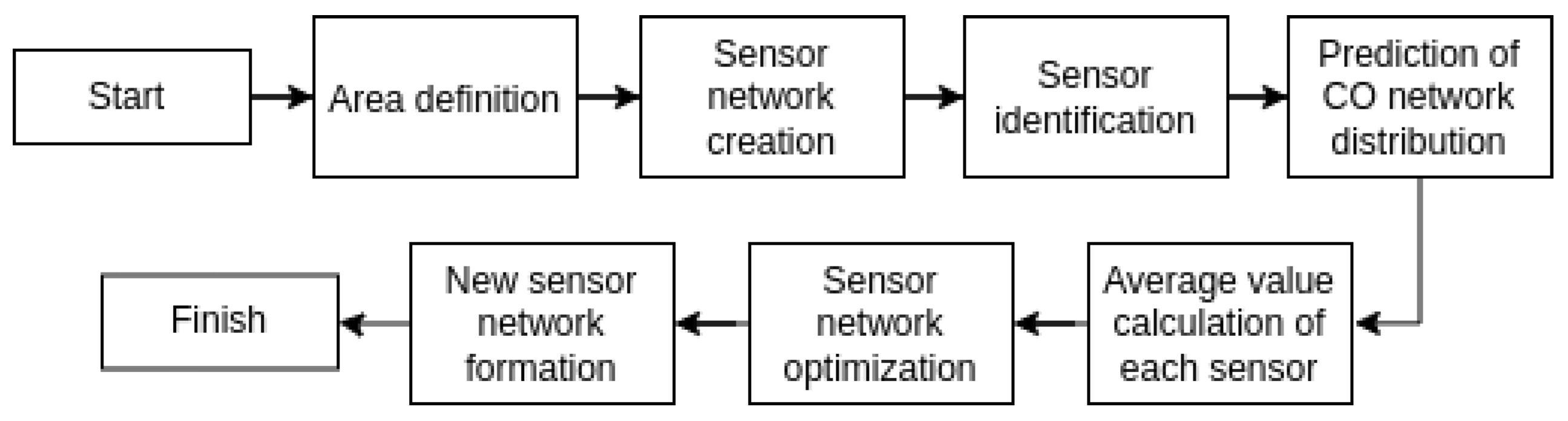
Figure 1 shows how this research was developed, from defining area coverage through to the formulation of a new sensor network, with each step outlined in more detail below:

• Definition of area: Initially, the region to be monitored by the sensor network was defined within the central part of the MRSP.
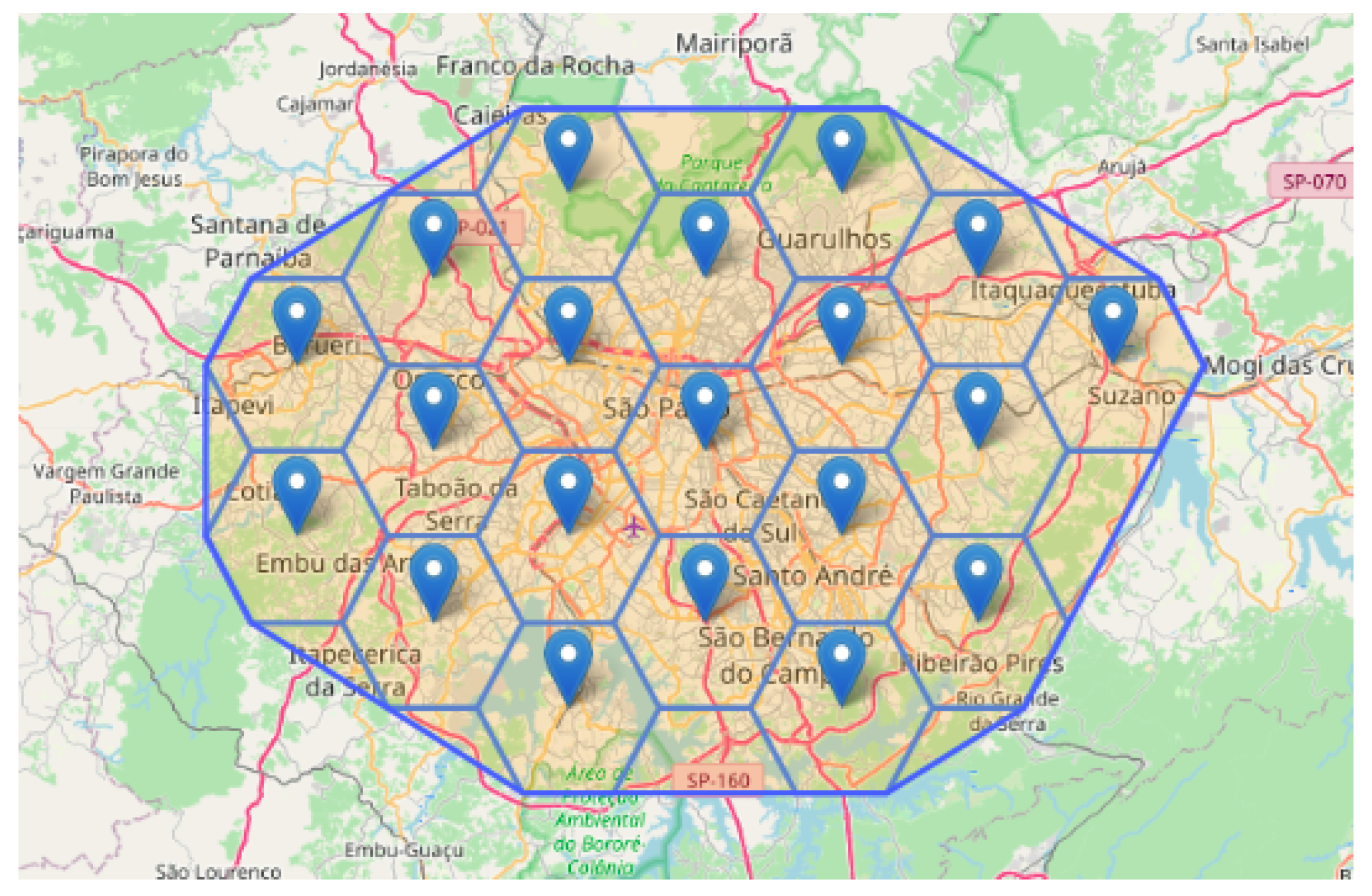
• Sensor network creation: In this step, the virtual sensor network is created to efficiently cover the entire defined area, as shown in Figure 2.
• Sensor identification: At this stage, each sensor receives an identification number to be used as a reference during network optimization.
• Prediction of CO network distribution: In this stage, measurements from physical sensors are used to calculate the linear regression model. Using IDW and INMET, the distribution of CO throughout the MRSP is then calculated using the Monte Carlo method.
• Average value calculation of each sensor: At this stage, the CO value of each virtual sensor is defined using the linear regression model and the IDW (based on INMET).
• Sensor network optimization: After defining the value of the virtual sensors, the group and route with the lowest variance are selected to optimize the sensor network.
• New sensor network formation: After selecting the ideal group and route, the new sensor network architecture is defined.

The method employs tessellation into hexagons in which a sensor is placed at the center of each cell. After an initial random distribution of cells obtained using Monte Carlo method, the presented algorithm is used to redistribute the cells in an optimal way concerning the number of used sensors. This is the core of this novel method and the São Paulo Metropolitan Region is used as a case.

The presented method to optimize the use of sensors to cover a given geographical area can be applied to any kind of sensor. The case study uses CO sensors, but the algorithm can accommodate NOx and particulate matter sensors as well with very few adjustments. In a smart city application, more complete data will be needed with more expensive sensors. This work contributes to make feasible the implementation of such network by decreasing its cost.

The rest of this article is organized as follows. Section 2 lists related works and Section 3 presents the main aspects of the hexagonal mesh sensor network. In Section 4, the structure and organization of the proposed algorithm are identified. Section 5 details minimizing the amount of CO sensors and in Section 6, the results and a discussion of each tested configuration are shown. Finally, Section 7 contains the conclusion of this article.

2. Related Works

Many related studies have researched wireless network strategies in the coverage and connectivity.

According to [7], the coverage of key points and network connectivity are two key issues related to wireless networks. Although some works [7] discuss mobile sensor deployment (MSD) aimed at improving the quality of coverage and connectivity, little attention has been paid to minimizing sensor movement, which in turn consumes sensor energy and substantially reduces their life. With this in mind, the authors of [7] addresses the problems of MSD and examines how to deploy them with minimal movement to create an WSN. The MSD problem is divided into two concerns: target coverage (TCOV) and network connectivity (NCON). Regarding the TCOV where sensor positioning is scattered, an exact algorithm based on the Hungarian method was proposed to create a near-ideal solution. This method was used to select the optimal sensors to move to those points. In the case of the heuristic TCOV algorithms, the standard algorithm was based on the Voronoi partition of the region deployment, intended to reduce the total movement distance of sensors. With regard to NCON, a solution based on the minimal Steiner tree was proposed, for which a combination of solutions for TCOV and NCON offer a promising answer to the original MSD problem, balancing the load of different sensors and prolonging network life.

In the scenario presented by [7], there was a concern with sensor load and positioning, but any reference to the minimization of sensors in any given area was omitted, introducing some algorithms from what the author proposed.

According to [8], sensor network deployment is one of the most studied subjects in the area of wireless sensor networks (WSN). This is in terms of selecting sensor locations within a specific region to maximize coverage and minimize deployment cost. A genetic algorithm was proposed to solve sensor deployment problem (SDP), using a variable-length genetic algorithm (VLGA). The authors of [8] state that this proposed method surpasses the existing approach of using a fixed-length genetic algorithm (FLGA) in terms of the quality of the results, speed of convergence and scalability. Furthermore, in this research, the authors of [8] reports that the VLGA approach results in lower deployment costs compared to data obtained using the FLGA approach.

Even though [8] addresses the coverage of the source and destination nodes, minimization of errors within the genetic algorithm was still not mentioned.

The authors of [9] demonstrate that autonomous network nodes can create adaptive wireless sensor networks, with great potential to improve and monitor real-world applications. For example, when an area is unknown and potentially unsafe, drones can operate in 3D environments, often allowing them to bypass debris and blocked passages to provide quick access and intelligence. Having faced these challenges, drones optimize device-to-device communication, deployment processes and available power supply for the devices and the hardware they carry. Aiming at finding a solution to this, the research on a bio-inspired self-organizing network (BISON) was presented, which uses the tessellation of Voronoi to achieve a desirable result. To improve this performance, there was an increase in (BISON) using a genetic algorithm, which improved network deployment time and overall coverage.

The research presented in [9] indicates it was not possible to solve the issue of an eventual power failure whilst achieving calibration in any given location. Coverage of node points was mentioned, but without addressing neither the overlapping of collection points nor the exact sensor location.

To improve sensor coverage, it is possible to define a sensor s as modeled at a point ps in space, and its detection region is represented using Euclidean coordinates centered on the ps. From this, many coverage problems were identified, such as ascertaining the maximum distance between sensors in the analyzed networks. It was observed that even when the least and most monitored paths use separate networks, there is no guarantee of separation of the Euclidean points elaborated on by [10].

Although [10] outlined the network node coverage problem, it was not sufficient for application to existing sensor networks. The authors of [10] approached it in an appropriate way, consistent with the Voronoi diagram. There were issues with unifying network protocols, such as location-based triangulation that requires at least three sensors to locate an object. In this research, the authors of [10] expected each point in S to be covered by at least three sensors.

According to [11], a location strategy based on connectivity and an evaluation of the Voronoi diagram resulted in an algorithm that eliminated isolated nodes and reduced redundant coverage, whilst maintaining network connectivity. With this, mobile nodes were directed to the best local positions according to the Voronoi partition.

Rooted in the quality issue of wireless sensor coverage, the authors of [11] proposed a deployment location strategy based on connectivity with the Voronoi partition to improve the performance of the monitoring network. However, this algorithm overlooked isolated nodes and reduced coverage redundancy to maintain network connectivity. These experimental results show that this algorithm guarantees greater network coverage and reduces node displacement [11]. However, the authors of [11] did not present a way to optimize and calculate the minimum number of nodes through decomposition techniques.

Monte Carlo method has been applied to sensor networks in both location [12] and energy balance [13] issues. In these references, the authors presented a systemic approach based on random numbers to achieve convergence in iterative algorithms at a convergence rate close to 1/N.

In [14], the Monte Carlo method was developed specifically to prevent failures. The approach is applicable to all apparatus triggered by change in temperature and humidity. It is of great importance to understand and refine the sensitivity of the many variables included when predicting typical failure rate in the field.

With coverage cited as one of the most important performance measures, the authors of [15] describe the applications of environmental and industrial monitoring by wireless sensors, when being monitored from a location far from the central base. The problem addressed by [15] concerns coverage complexity, and random deployment is seen as a simple way to deploy sensor nodes. However, at the same time, it can cause unbalanced deployment. To solve this problem, the authors of [15] proposed a genetic algorithm using a normalization method (Monte Carlo), to predict an efficient evaluation where computation time was reduced without loss in quality of the solution used. Additionally, this method began with a small number of random samples and consecutively increased the number of each subsequent sample.

Although [15] mentions that the study can be improved by agreeing locally on the generic algorithm and comparing it with other existing methods, it is not sufficient for current application with a GA. The random combination presents overlapping points, which can cause the points established by the sensor algorithm not to be reached. In addition, the minimization of predicted points was also not addressed.

Consequently, the current research shows different views of sensor optimization techniques. Most authors use traditional methods to optimize the distribution of network nodes, such as the previous works presented in this section.

Regarding the detection of divergent values supported by a genetic algorithm, the authors of [16] suggest that several types of sensor data can be calculated by IoT. For this it proposes the use of a one-class support Tucker machine (OCSTuM), which seeks to support unidentified errors in the vector type of tension areas of multiple sensor data sets. This method retains the underlying data information, improving the accuracy and efficiency of error detection. The GA is used to select a subset of the data sensor assets, which searches for ideal simultaneous GA-OCSTuM model parameters including the following: chromosome code; fitness function; selection operator; crossover operator; and mutation operator.

According to [17], wireless sensor networks collect and transfer environmental data from a predefined region to a central station for processing, analysis, and forwarding. Considering there are a number of sensors with different detection ranges, the issue of maximizing coverage is known for its complexity, as the prevailing methods generally rely on meta-heuristic techniques through estimated fitness functions. That said, the authors of [17] present a new, efficient, alternative meta-heuristic genetic algorithm, which overcomes several vulnerabilities of existing ones, together with an exact method for calculating the fitness function for the highlighted issue. The proposed genetic algorithm includes a heuristic process at the point of beginning population. It also calculates exactly the entire proposed area for the fitness function and a combination of the Laplace and arithmetic crossover method operators. Experiments were conducted to compare the proposed algorithm with five state-of-the-art methods across a wide range of problem occurrences. For the majority of the occurrences tested, the results indicate that the algorithm offers the best performance in terms of the solution’s quality and stability.

According to [18], communication within IoT applications via WSN requires substantial energy use. It also suggests that a genetic algorithm with a dynamic clustering approach is a very effective technique to conserve energy throughout the design and planning process of an IoT network. Therefore, dynamic clustering defines a head cluster (HC) with higher energy for network data transmission. In this research, dynamic clustering methodology and frame relay nodes were employed to select the chosen sensor node from among the cluster nodes.

This approach also results in a reduction of the overall number of sensors, whilst maintaining a higher number in network regions of greater variation, as well as CO distribution in the MRSP, developed from the Monte Carlo method.

According to [19], the technique to be used for the sensors is viable and effective. Additionally, it is more efficient and maintains load balancing, aiming to increase the lifespan and scalability of networks. Based on criteria such as distance and density, a GA that improves energy consumption is simulated to develop the functioning capacity of sensory network nodes. The developed protocol works as a static model on multiple levels with the deployment of nodes to optimize energy and distance between sensory points during network operation.

The research presented in [20] mentions that spacetime data fusion is an inexpensive way to produce high-resolution remote sensing images using graphical data from varied sources. However, the large computational complexity of flexible spatiotemporal data fusion FSDF prevents its use in large-scale applications. Moreover, the field of FSDF decomposition strategy generates loss of precision at the subdomain boundaries, when taking into account the effects of edges. Therefore, a new study is proposed to reduce this computational complexity, the main improvement being the replacement of the TPS interpolator with accelerated inverse distance weighting IDW.

In line with [21], (WSN) energy resource is limited when employing network nodes. A complex routing challenge is created and it is necessary to observe factors such as: data collection and aggregation; network lifespan; and (WSN) stability and capacity. These are some parameters that must be be maximized according to the constraints of these specifics. Clusters of heterogeneous wireless sensor networks have not been much explored. Thus, it is necessary that they be enhanced to unlock the potential of WSN networks.

The research presented in [21] presents a classical benchmark functions algorithm, which harnesses the residual energy of sensor nodes and results in acceptable energy consumption. However, the distance traveled covered between X and Y must be optimized to minimize acceptable network operation.

Nonetheless, according to [22], a minimal number of wireless sensor node is able to become smart farming without removed coverage to reduce cost. The lifetime of the sensor nodes has to be expanded by applying an energy-efficient algorithm or some other techniques. Therefore, an appropriate node deployment scheme combined with an energy-efficient routing algorithm can reduce the complexity of problems, such as routing, network communication, and data aggregation by minimizing the number of sensors needed. The multiple-input multiple-output technique is used to enhance the data rate of sensors by compressing fading effects and interference. A trustworthy model is also considered here to protect the routing protocol by segregation the malicious nodes.

The authors of [23] created a novel hybrid method based on two modern meta-heuristic algorithms in order to solve dynamic data replication problems in the fog computing environment. In the proposed method, the authors present a set of objectives that determine data transmission paths, choose the least cost path, reduce network bottlenecks, bandwidth, balance, and speed data transfer rates between nodes in cloud computing.

In [24], the employs and mode of the data replication problem are designed as a multi-objective optimization problem that considers the heterogeneity of resources, least cost path, distance, and applications based on replication requirements. Firstly, a new hybrid meta-heuristic method, using the arithmetic optimization algorithm (AOA) and the salp swarm algorithm (SSA), is proposed to handle the problem of selection and placement data replication in fog computing.

A comparison of the presented method to the previously published algorithms is shown in

Table 1. Comparison of sensor network organization methodologies in coverage and connectivity area.

Author	Advantage	Disadvantage
Zhuofan Liao et al. [7]	Network connectivity, Quality of coverage, Prolonging network life	Minimizing sensor, Sensor energy
Dina S. Deif and Yasser Gadallah [8]	Maximize coverage, Existing approach, Speed of convergence, Scalability	High cost, High response time
Khouloud Eledlebi et al. [9]	Autonomous network, Monitor real applications, Quick access and intelligence, Overall coverage	Power supply, Power failure, Overlapping of collection points, Calibration
Anthony Man-Cho So and Yinyu Ye [10]	Sensor coverage, Distance between sensors	Ascertaining the maximum distance, No guarantee of separation, Unifying network protocols
Qihua W. et al. [11]	Connectivity, Eliminated isolated nodes, Reduced redundant coverage	Low performance, Low monitoring network, Way to optimize
Martin Vins and Martin Sirovy [13]	Sensor networks, Convergence in iterative algorithms	Energy balance
Jonathon Tucker et al. [14]	Prevent failures, Apparatus triggered in temperature and humidity, Predicting typical failure	High response time
Yourim Yoon and Yong-Hyuk Kim [15]	Performance measures, Normalization method, Efficient evaluation	Coverage complexity, Random deployment, Unbalanced deployment
Nguyen Thi Hanh et al. [17]	Maximizing coverage, Efficient, alternative meta-heuristic, Quality and stability	High complexity, High vulnerabilities
Shalli Rani [18]	Dynamic clustering approach, Effective technique, Conserve energy	Substantial energy use, Greater variation
Aridaman Singh Nandan [19]	Load balancing, Scalability of networks, Energy consumption	High network operation
Huan Gao et al. [20]	High-resolution remote, Accelerated IDW	Large computational complexity, Rates loss of precision
Sumika Chauhan [21]	Energy consumption, Network operation	Energy resource is limited, Complex routing
Sathian Dananjayan et al. [22]	Wireless sensor node, Energy-efficient	High cost, High complexity
Ahmed Awad Mohamed et al. [23]	Dynamic data replication, Computing environment, Transmission paths	Speed data transfer rates
Ahmed Awad Mohamed et al. [24]	Hybrid meta-heuristic method, Placement data replication, High fog computing.	Data replication problem

, highlighting the advantages of the former.

3. Hexagonal Sensor Network Mesh

This section will describe the implementation of a hexagonal sensor network mesh and explain the FGR technique. Following, CO concentration and normalization equations will be demonstrated, as well as calculations of the predicted values using Equation (2) to estimate a CO value.

In this research, temperature and humidity are used to estimate the CO level in a given cell. The effect of the wind has influence in the pollution level and, therefore, in readings of the sensor. However, it is very complex to model this effect and include it in the sensor network modeling. For this reason, the proposed algorithm deals with the instantaneous output of the sensors and does not consider the influence of the wind.

The geographical distribution of sensors is performed under the assumption that all sensors are capable of covering the area of the cell it is located on. All sensor distribution algorithms are developed under this constraint. Therefore, the presented method is agnostic concerning the nature of the sensor and its positioning, provided the assumption is satisfied. For the case study, a sensor board based on an ESP8266 microcontroller and a MQ7 CO sensor was developed. These boards were positioned as public posts at different heights.

The sensor network is composed of virtual sensors with data predicted using the IDW method and applied to an INMET database that provides temperature and humidity measurements at different locations in the state of São Paulo, in conjunction with a mathematical model that calculates CO from patterns found in the measurements of physical sensors.

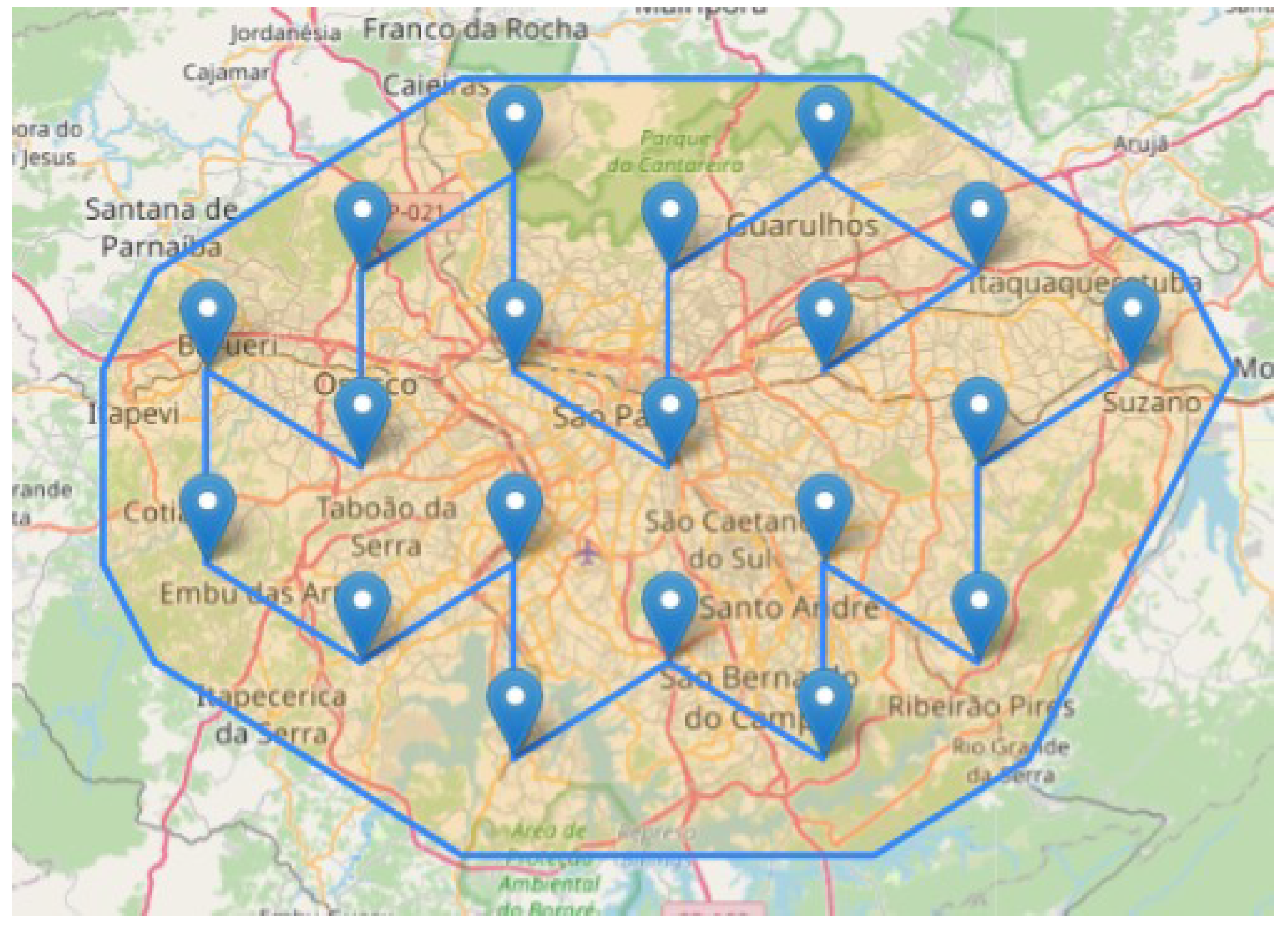
Through computer simulations, a hexagonal sensor network mesh has been designed to extend the respective coverage area throughout the studied region, as shown in Figure 2.

To calculate and create the geographic areas, the minimum number of sensors and their respective locations must first be established. Using Equation (1) to formulate the suggested structure, 3 physical sensors were used to actively perform data collection 24/7, with another 20 sensors randomly assigned throughout the MRSP.

The purpose of replacing the CO network sensors with the least resultant quantity is to assess the feasibility of minimizing the number of these in each geographic area. By identifying the least number of CO sensors needed to cover an area, a consequent power reduction of 560 mW per sensor is achieved.

Data recorded by the physical sensors demonstrates a correlation between temperature, humidity, and CO, illustrated in

Table 2. Correlation between temperature, humidity, and CO.

	Latitude	Longitude	Temperature	Humidity	CO
Latitude	1.0	0.013	−0.048	0.0075	−0.048
Longitude	0.013	1.0	−0.089	−0.058	0.078
Temperature	−0.048	−0.089	1.0	0.016	0.96
Humidity	0.075	−0.058	0.016	1.0	−0.27
CO	−0.048	0.078	0.96	−0.27	1.0

. This enables the creation of a mathematical model that measures the value of CO through temperature and humidity, as shown in

Table 3. Mathematical model that measures the value of CO through temperature and humidity.

Dependent Variable	Method	Independent Variables	Linear Equation	${\mathit{R}}^2$	Prob (F-Statistic)
$CO$	Least squares	T e H	$CO=1.9 T-0.3 H+10$	1.0	0.0

and Equation (1), where $C{O}_{concentration}$ indicates the concentration of carbon monoxide in particles per million (ppm), T the temperature in °C, and H the relative humidity.

$$C{O}_{concentration}=1.9T-0.3H+10,$$

(1)

In this research, the data values of CO, temperature, and humidity are provided by three physical sensors distributed geographically in the MRSP. These data are used to calculate an equation that predicts CO using the method of least squares, and the 20 other previously calculated random sensors. Consequently, the temperature and humidity data from INMET’s temperature and humidity records were used as climatological measurement units for Equation (1) to define CO distribution in the MRSP.

To predict CO in particles per million (ppm) in locations not covered by physical sensors, the numerical method of spatial interpolation called IDW was employed. This technique is intended to predict the value of a variable ĥ($z_0$), based on the sum of the selection of values from h($z_i$), weighted by the coefficients $\lambda$($z_0$), as indicated by Equation (2) and presented by [25].

$$\widehat{h}\left(z_0\right)=\sum _{i=1}^N{\lambda }_i\left(z_0\right)h\left(z_i\right)where\sum _{i=1}^N{\lambda }_i\left(z_0\right)=1$$

(2)

Using Equation (3) as a basis and using CO measurement of the $z_1$ coordinate as a reference, CO value of the $z_0$ coordinate can be estimated. Accordingly, Equation (3) can be defined using Equation (2).

$$\widehat{CO}\left(z_0\right)=\sum _{i=1}^N{\lambda }_i\left(z_0\right)CO\left(z_i\right)where\sum _{i=1}^N{\lambda }_i\left(z_0\right)=1$$

(3)

As per Equation (4), each coefficient $\lambda$($z_0$) is given by means of the weight quotient $w_i$($z_0$) using the sum of all the other coefficients. Every weight $w_k$($z_0$) indicated in Equation (5) is obtained using the inverse of the vector distance defined by $d^{{}^p}$($z_0,z_k$)${}^{\mu }$, where $z_0$ and $z_k$ are the Cartesian coordinates of ĥ($z_0$), respectively. This is to predict Cartesian coordinates of h($z_1$) and to calculate their $w_k$($z_0$) and $\mu$ with the purpose of decreasing the data coefficient with the longest vector distance of ĥ($z_0$) [25].

$${\lambda }_i\left(z_0\right)=\frac{w_i\left(z_0\right)}{{\sum }_{k=1}^N{w}_k\left(z_0\right)}$$

(4)

$$w_k\left(z_0\right)=\frac{1}{d^{{}^p}{(z_0,z_k)}^{\mu }}$$

(5)

However, to estimate the CO value in any given region, the Cartesian coordinates of $z_0$ must have two directions: one horizontal (latitude) and the other vertical (longitude). Thus, the vector distance $d^{{}^p}$($z_0,z_k$)${}^{\mu }$ in Equation (5) is calculated using Equation (6), where $x_0$ and $y_k$ are the latitude and longitude of ĥ($z_0$), and $x_0$ and $y_k$ are the latitude and longitude of h($z_i$), respectively, as shown by [25].

$$d^{{}^p}{(z_0,z_k)}^{\mu }={\left(\sqrt{{\left(x_0-x_k\right)}^2+{\left(y_0-y_k\right)}^2}\right)}^{\mu }$$

(6)

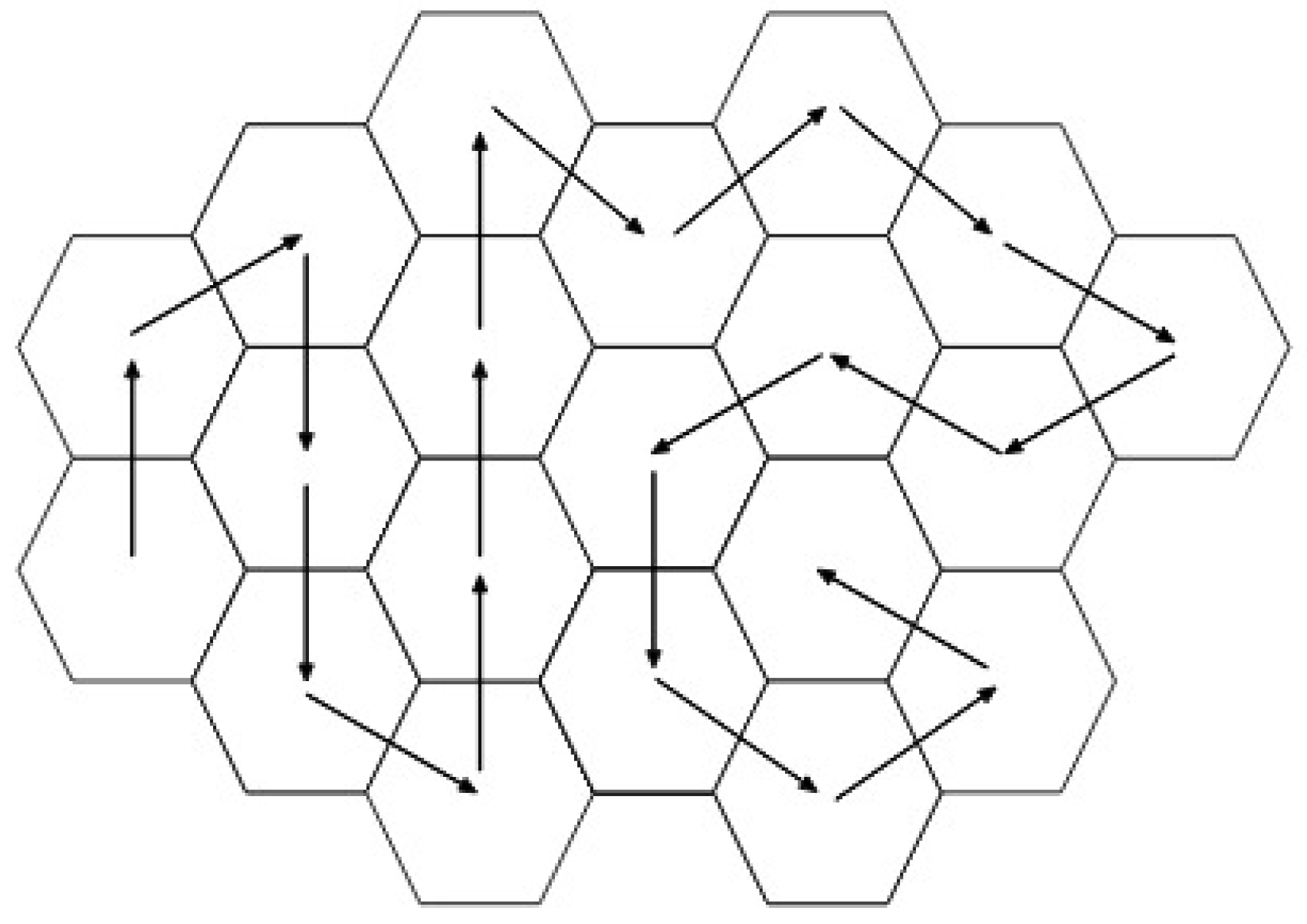
This research proposes to elaborate a route that goes through all the sensors (route), and fragment it into smaller regions (groups), replacing the sensors in these regions with a single point to cover each area. To reduce any errors in sensor location regions, a GA was constructed to establish a route and set of groups with the smallest possible variance.

In order to minimize the sensor network and conserve the main characteristics of CO distribution through FGR, developmental computation through a genetic algorithm was chosen, as the sensor locations resulting from the minimization would favour the most relevant areas within the MRSP. To establish these areas, a path (route) that ran through all the sensors in the network was chosen, as shown in Figure 3.

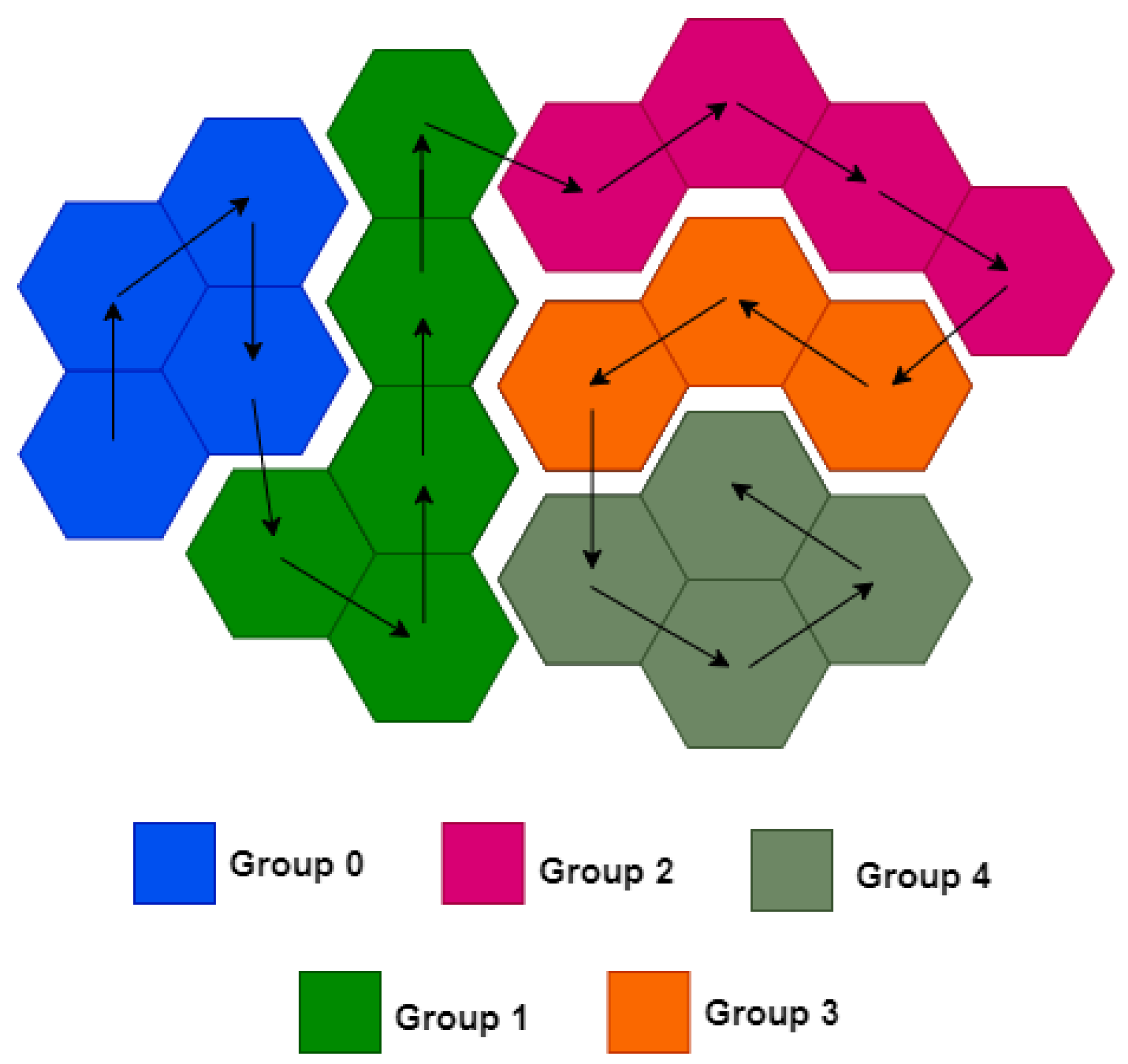
To analyze the most relevant areas of the route, it was decided to fragment the sensor network into smaller sub-regions called groups. Figure 4 illustrates this procedure.

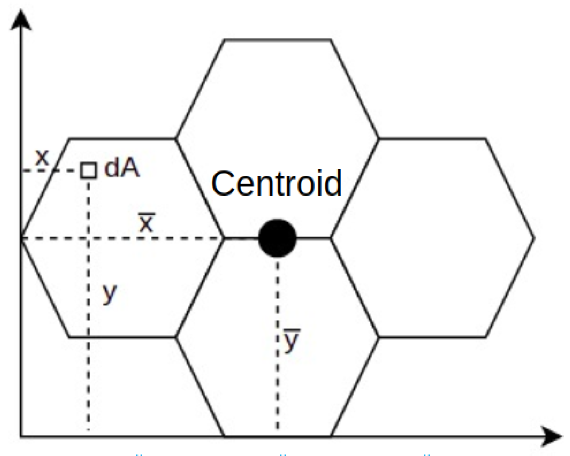
As illustrated in Figure 4, once the groups have been formed, the resulting sensor location is calculated from the centroid of each group’s coverage area. According to [26], the centroid of an area can be defined as the Cartesian coordinate [$\overline{x}$,$\overline{y}$], calculated at that moment. The result is the total of each area’s particles dA calculated by their respective distances $\tilde{x}$ and $\tilde{y}$, which make up one or more areas in question, and then divided by the total area ${\int }_{A}dA$, as illustrated in Figure 5 and by Equation (7).

$$\begin{array}{c}\hfill \overline{x}=\frac{{\int }_A\tilde{x}dA}{{\int }_{A}dA}\overline{y}=\frac{{\int }_A\tilde{y}dA}{{\int }_{A}dA}\end{array}$$

(7)

To estimate the significance of any given group, variance was selected as an indicator of data dispersion between group sensors, suggesting little variation existed between sensors. The average error was directly proportionate to the indicator, as shown in Equation (9). Here, n represents the amount of data, otal of each area’s particles dA calculated by their respective distances x, the data of the entire sample area, and ${\overline{x}}_{obs}$ the average of these as described in Equation (8) and defined by [27].

$${\overline{x}}_{obs}=\frac{1}{n}\sum _{i=1}^{n}x$$

(8)

$$va{r}_{obs}=\frac{1}{n}\sum _{i=1}^n{(x-{\overline{x}}_{obs})}^2$$

(9)

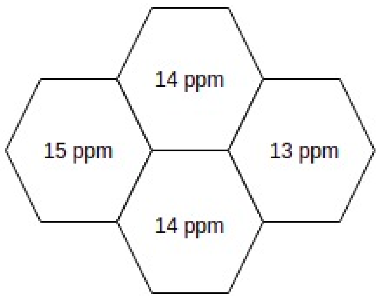
Using these concepts to calculate the dispersion of CO in a group, Equation (9) can be rewritten according to Equation (10), where CO indicates the value predicted by (IDW) for any given sensor, ${\overline{CO}}_{obs}$ the average values of CO sensors of the group, and COobs their variance. Therefore, it is possible to calculate the dispersion of the group illustrated in Figure 6 through Equation (10), as seen by the result in Equation (11).

$$C{O}_{obs}=\frac{1}{n}\sum _{i=1}^n{(CO-{\overline{CO}}_{obs})}^2$$

(10)

$$C{O}_{obs}=0.5\mathrm{ppm}$$

(11)

Using Equation (10), the dispersion of the route can be calculated through the sum of the dispersions in each group. Using Equations (12) and (13) to arrive at a resolution, a greater dispersion in groups 1, 2, and 4 can be seen in Equation (12), as they presented greater $C{O}_{obs}$ than other groups.

$$Sum=\sum _{j=1}^{len\left(A\right)}\sum _{i=1}^{A_j}\frac{{(C{O}_i-{\overline{CO}}_{Aj})}^2}{A_j}$$

(12)

$$\begin{array}{cc}\hfill C{O}_{obs}& \left(GROUP0\right)=0.68\mathrm{ppm}\hfill \\ \hfill C{O}_{obs}& \left(GROUP1\right)=1.36\mathrm{ppm}\hfill \\ \hfill C{O}_{obs}& \left(GROUP2\right)=1.25\mathrm{ppm}\hfill \\ \hfill C{O}_{obs}& \left(GROUP3\right)=0.66\mathrm{ppm}\hfill \\ \hfill C{O}_{obs}& \left(GROUP4\right)=1.18\mathrm{ppm}\hfill \\ \hfill & Sum=5.15\mathrm{ppm}\hfill \end{array}$$

(13)

The result obtained through Equation (13) (resolution) indicates the total dispersion of sensors present in the groups indicated in Figure 7’s example. From this, the genetic algorithm has the final objective of matching the groups and routes, resulting in the smallest sum of sensor network variances, indicated in Equation (12).

The purpose of this article is to present a novel technique of minimizing the number of sensors needed to cover a given geographic area. For this purpose, the region under scrutiny is split in hexagonal cells and a genetic algorithm is applied to minimize the number of required sensors.

4. Structure and Organization

In this section, details regarding the structure and organization of the FGR technique will be explained. To achieve the proposed objectives, it is necessary to address the main concepts that constitute their respective applications in this research, including the following:

• Individual: Any system input that could become a possible solution to the problem at hand. From this concept each pair constituted by a set of groups and a route (chromosome group and chromosome route) forms a possible solution to minimize the sensor network [28].
• Population: A collection of individuals, i.e., a number of pairs consisting of a route and a set of groups [28].
• Allele or Locus: Indicates a position within a chromosome, as shown in Figure 8 [28].
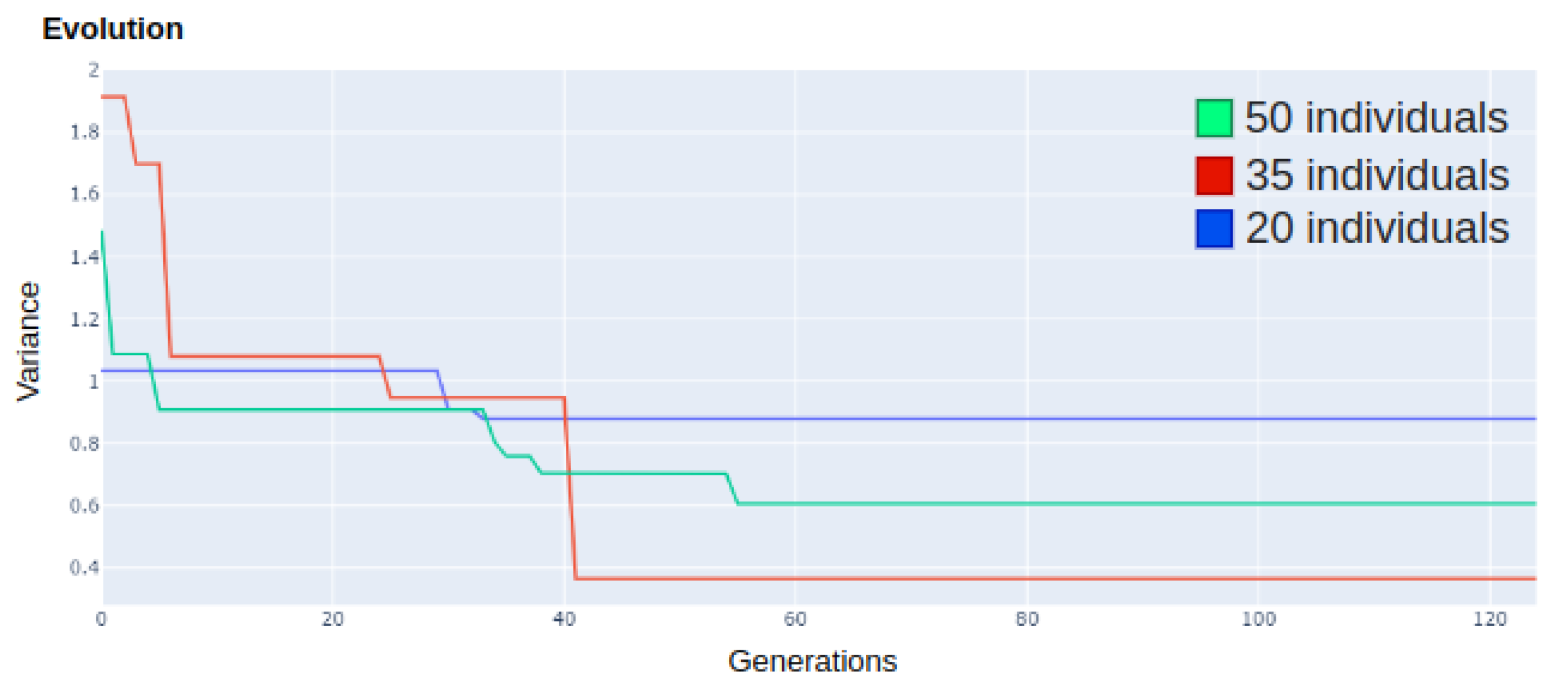
• Generations: Term to quantify the improvements achieved among all individuals of a population [28].
• Elitism: Name given to the process where characteristics of an individual remain unchanged within a generation [28].
• Elitism rate: Coefficient that indicates what percentage of the population should be kept unchanged [28].
• Chromosome: Defined as any data that has the characteristics of an individual [28]. Based on this, each individual must have the following two chromosomes:

  -

  Chromosome group: Indicates a set of groups that make up the sensor network.

  -

  Chromosome route: Indicates a route.

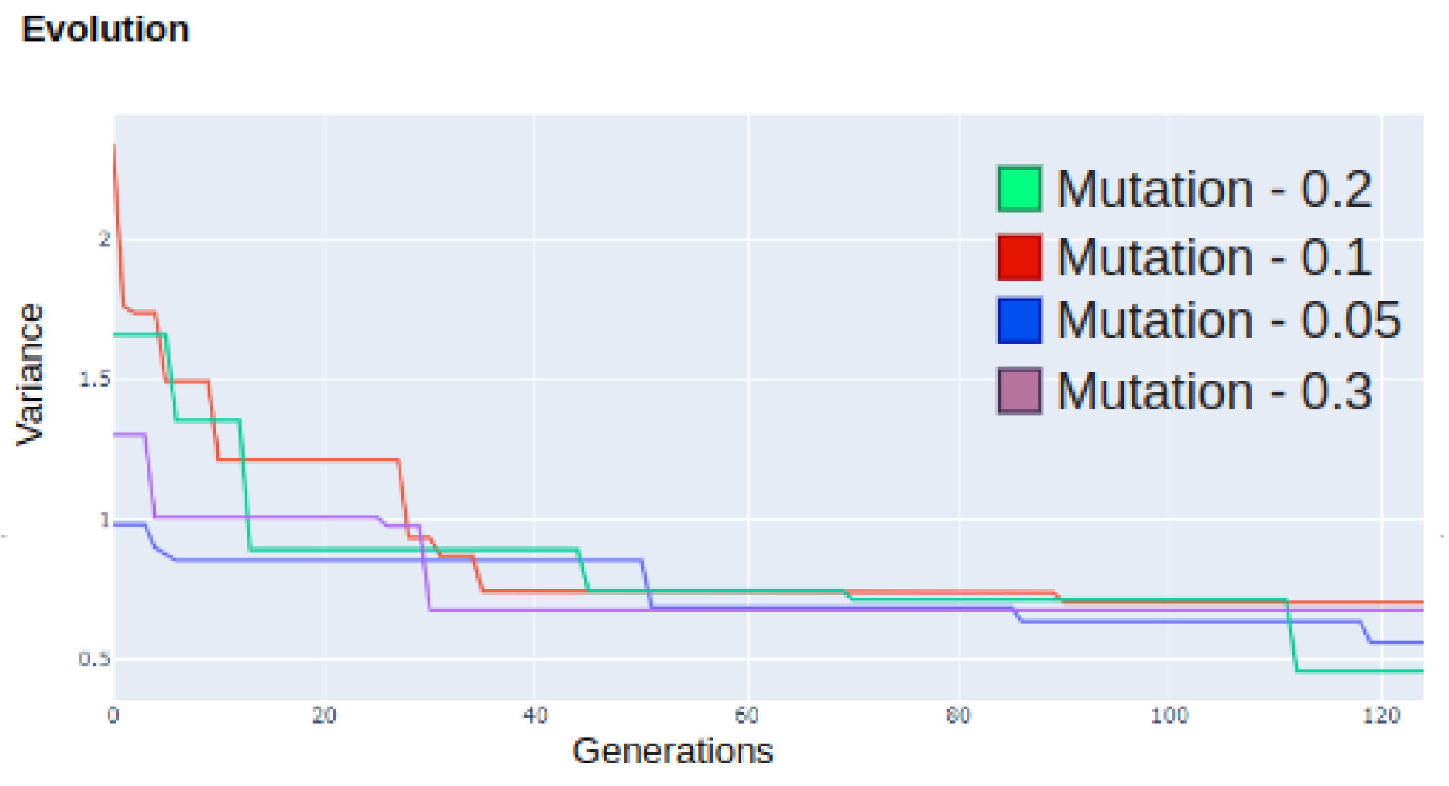
• Evolution: Process responsible for making changes to chromosomes, with the objective of finding the best possible solution for the problem in question. In this work, ref. [28], recombination techniques were not used.
• Mutation: Occurs when there is a random change in the chromosomes of an individual [18].
• Mutation Rate: Coefficient that indicates the probability of mutation occurring within the chromosomes of an individual [18].

As Figure 7 illustrates, the hexagons (which represent the coverage area of each sensor) are numbered from the top-left to the bottom-right-hand side of the image. The numeration was defined in compliance with the collected CO data, taking into account the geographic area.

In this work, the GA presents two chromosomes, one for the group and another for the route. The length of the group chromosome varies under a controlled fashion. Once the maximum and minimum values of sensors per group are defined, the algorithm increases the length in integer increments until it reaches the number of sensors in the network. This happens because the number of alleles in a chromosome is equal to the number of sensors contained in each group. Figure 9 illustrates the number of sensors belonging to a particular group. To create this chromosome, Algorithm 1 was used, as will be explained next.

Algorithm 1 Separation by groups

1: while SUM(group) != NS do 2:      N_num <- number_random(max_S,min_S) 3:      if $SUM\left(group\right)+N\_num<=NS$ then 4:             group.increase(N_num) 5:      else 6:             group.increase(NS-SUM(group)) 7:      end if 8: end while

In Algorithm 1, the variable NS in line 1 represents the number of sensors in the architecture. In this case, while the sum of all numbers contained within the chromosome group is different from NS, it is concluded that the chromosome has not yet managed to extend through the entire architecture. To avoid creating some groups with an excessive amount of sensors and others with a minimum amount, the algorithm alternatively chooses a random number indicated by the variable N_num, within the maximum and minimum limit of sensors per group indicated, respectively, by max_S and min_S in line 2. In other words, the user defines the minimum and maximum number of sensors per group. Using this definition, the algorithm calculates the distribution with the lowest possible variance.

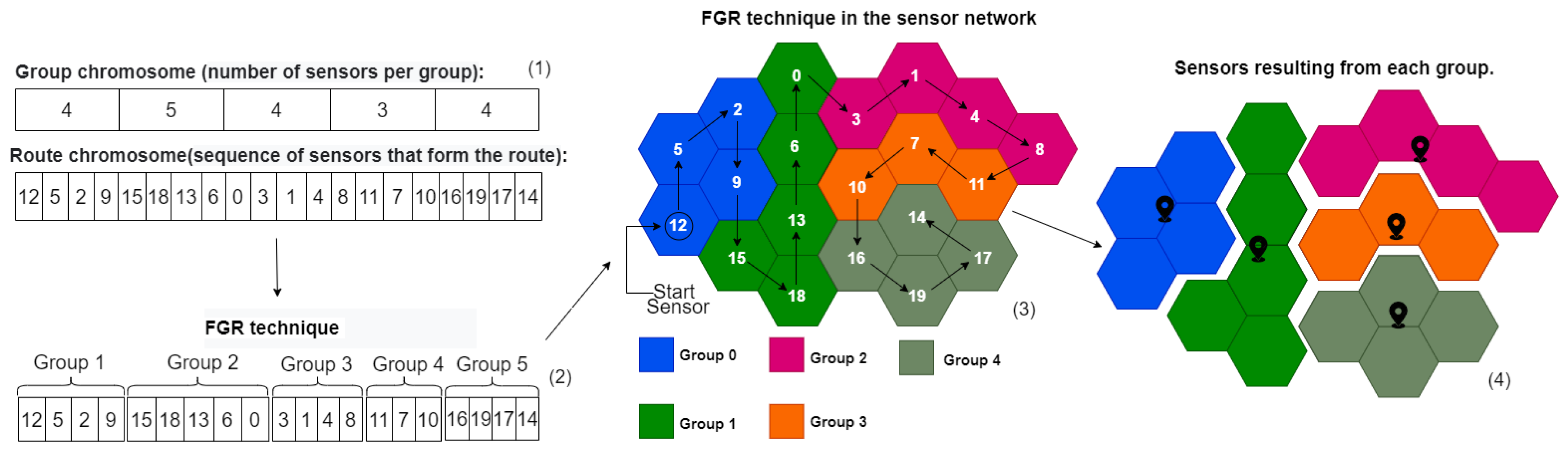
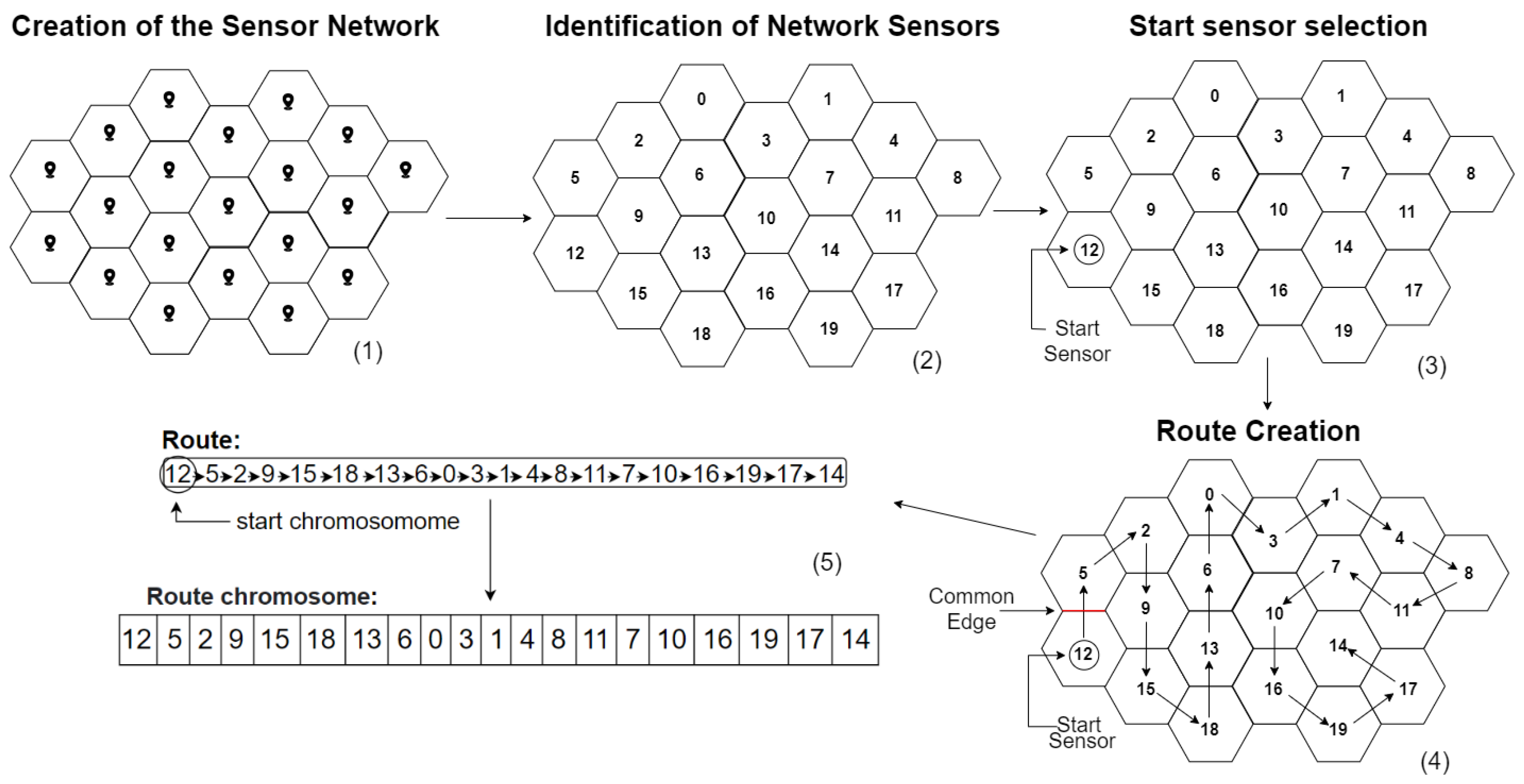
The length of the route chromosome is the number of sensors in the overall network as the route must pass through all sensors, the composition is developed from identifiers provided for each sensor in the structure, illustrated in Figure 10(2). The position of each allele indicates the sequence of sensor indentifiers added to the route during the development process, starting with the sensor that indicates the first position of the route, as shown in Figure 10(3). Each sensor n at a specific position in the route has an edge in common with the next sensor of the sequence, as shown in Figure 10.

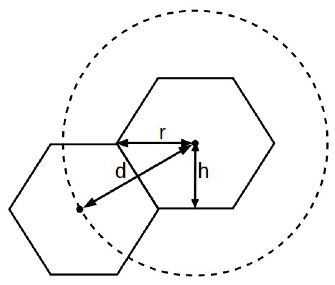
Each hexagon has a distance, d, which separates it from neighboring hexagons. Such a distance can be described by Equation (14), which is used to find the neighboring hexagons to the polygon in question, as described in Figure 11.

$$\begin{array}{cc}\hfill & h=\frac{r\sqrt{3}}{2}\hfill \\ \hfill & d=2h\hfill \\ \hfill & d=r\sqrt{3}\hfill \end{array}$$

(14)

r = hexagon edge

The second step of FGR is to create the chromosome route. The following two assumptions are made:

• The chromosome route must have a length equivalent to the number of sensors.
  All sensors in allele n + 1 must have an edge in common with sensor n, as shown in Figure 10(4).
• The chromosome route cannot contain duplicate sensors.

With these assumptions, it is suggested that each chromosome route created by the algorithm contains all the sensors indicated by the hexagons illustrated in Figure 2 (approximately 20 hexagons). To avoid repetition of sensors during route creation, Algorithm 2 was developed, which has the function of creating the chromosome route. According to these assumptions, Figure 10(4) illustrates a route model that can be developed from the algorithm.

In line 2 of the same pseudocode, the while instruction ensures that all routes have a size equivalent to the number of sensors (assumption 1). To ensure that assumption 2 can be met, the algorithm tries 12 times (line 4) to select a different network sensor (line 8) with an edge in common with the sensor in the last position of the route (line 3).

If the chosen sensor is not yet part of the route, it is added to it (line 9) and this sensor becomes the last sensor of the route.

If the algorithm does not find any sensor that is not already on the route during all attempts (line 6), it chooses to exclude the last sensors that were added to the route (line 18). For this, a return variable is declared (line 1), which indicates the number of sensors in that route to be excluded. In order to prevent this being repeated indefinitely, the value of this variable is increased (line 16) when it is required consecutively.

In case there is an error caused by a return variable with a value greater than the length of the route (line 19), it is initiated only with a randomly selected sensor (line 20) and the return variable is re-initiated with an indicated value on line 1 (line 21).

To prevent the variable in line 1 from experiencing excessive growth in its value and causing a large number of restarts as sensors are added to the route, this variable either has its value reduced (line 10) or reset to an initial value indicated on line 1 (line 11).

Algorithm 2 Route Creation

1: return <- 2   2: while SIZE(route) != number_of_sensors do   3:       sensor <- route.last   4:       for $iteration=1,2,\dots ,12$ do   5:             select a random neighbouring sensor   6:             if $neighbourINSIDE\_OFroute$ then   7:                    pass   8:             else   9:                    route.add(sensor) 10:                    return - - 11:                    return <- MAXIMUM(2,return) 12:                    end for 13:                    continue 14:             end if 15:       end for 16:       return <- return + 3 17:       if $LENGTH\left(route\right)>return$ then 18:             route.delete(last_return_sensors) 19:       else 20:             route <- LIST[select a random sensor] 21:             return <- 2 22:       end if 23: end while

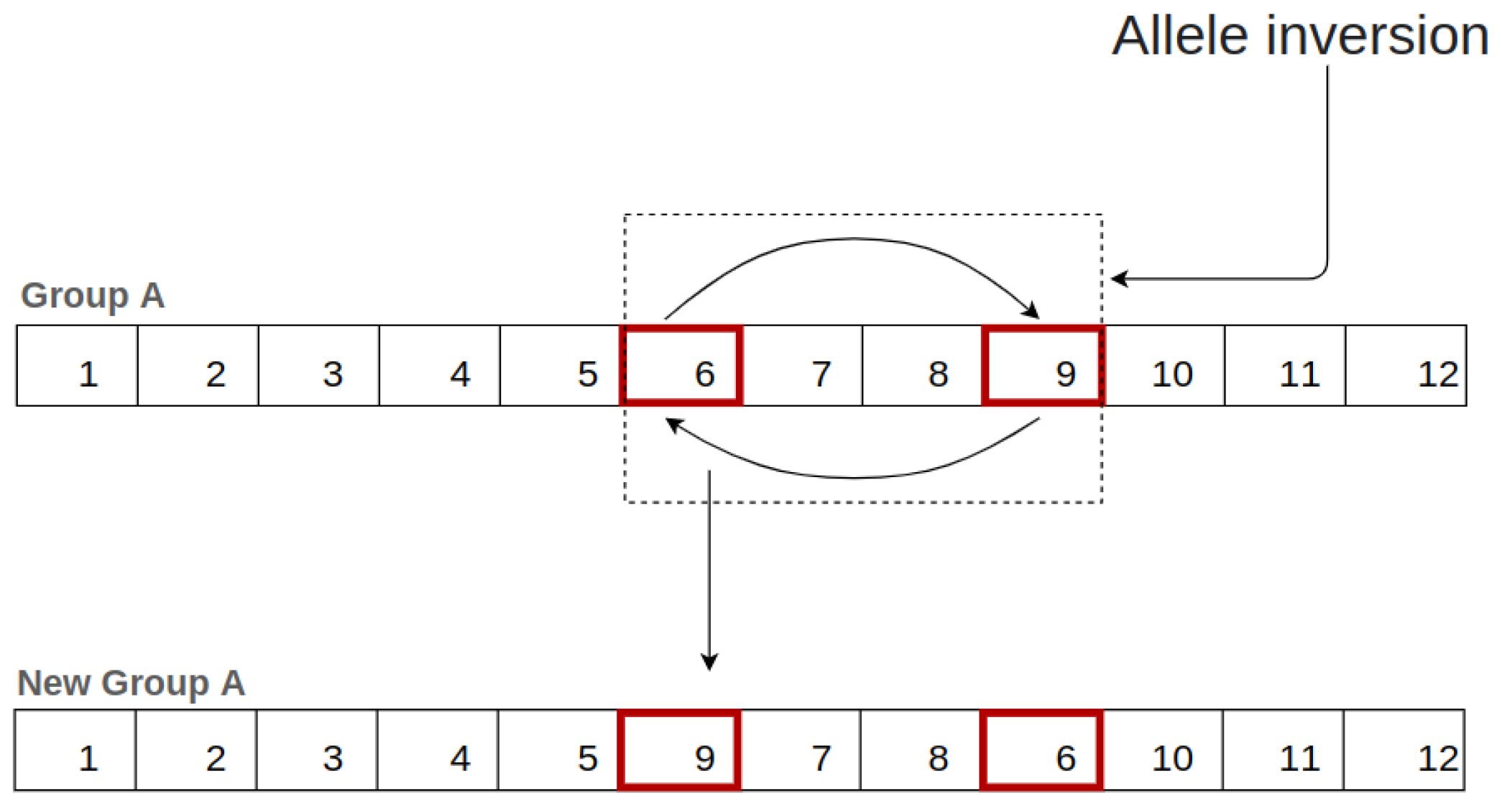
For the reconstruction of chromosome groups and routes, two strategies were selected, the first strategy being applied only to the chromosome group.

This strategy inverts the position of two groups within the chromosome, so there is no change in the total number of sensors. However, the inversion between the positions reorganizes the sensor groups in their respective chromosome route, changing their variance as illustrated in Figure 12.

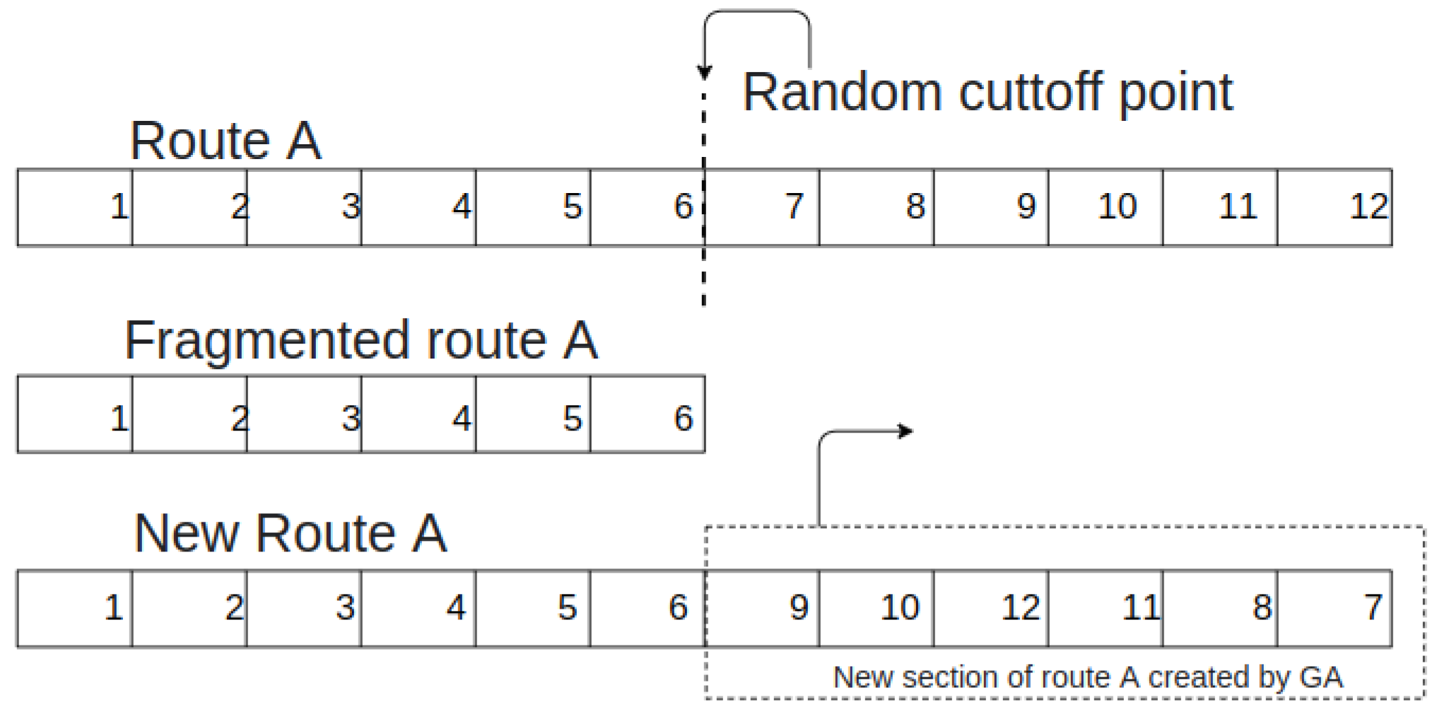
The second development strategy has application for both group and route. Should this technique randomly fragment through development Algorithms 1 and 2, a new chromosome group or route is produced (Figure 13).

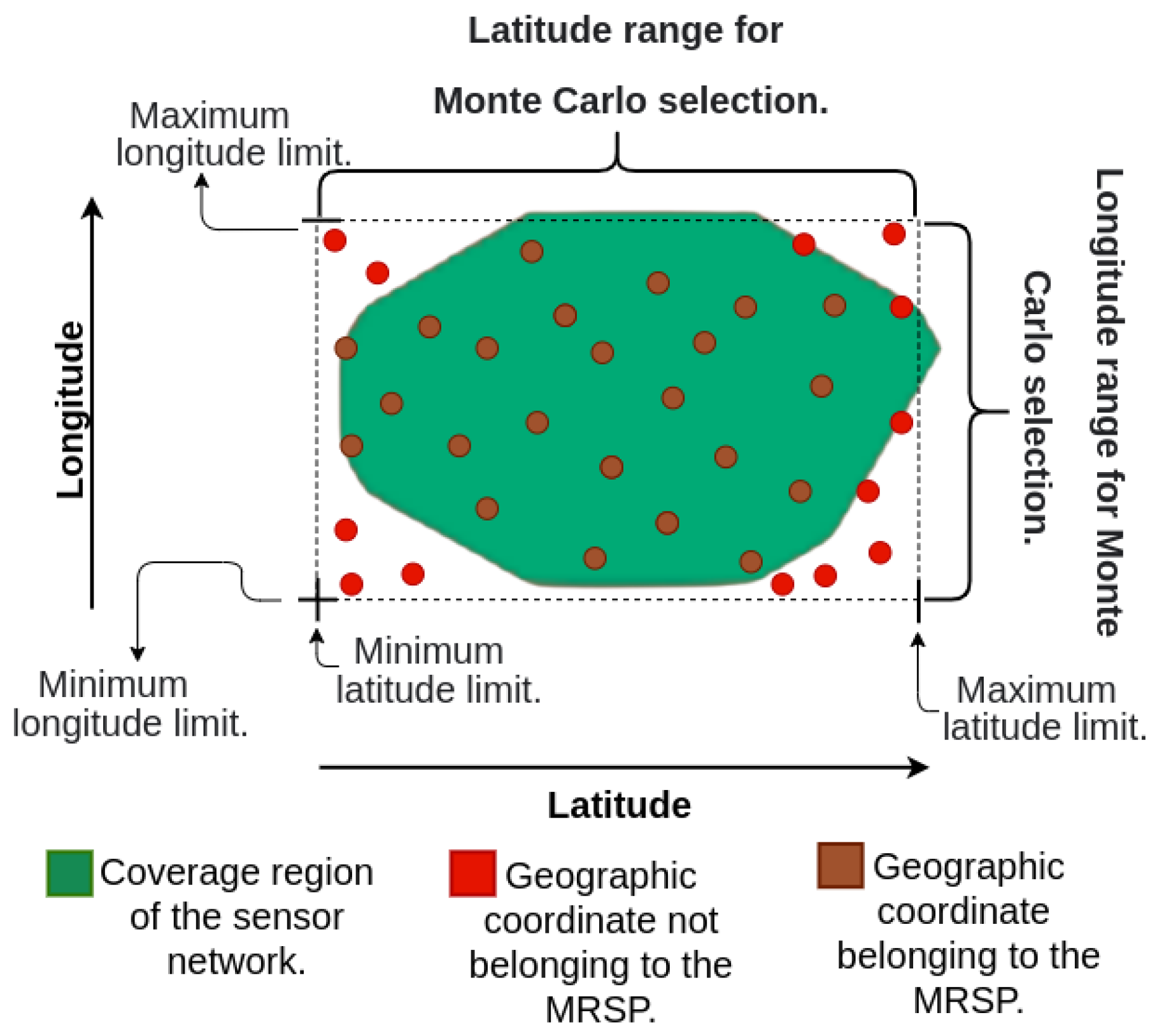
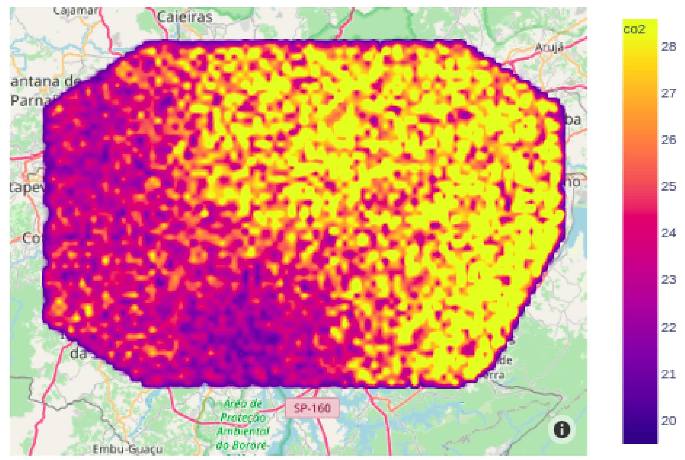
To predict the distribution of carbon monoxide throughout the MRSP in a thorough and more detailed way, the numerical method IDW was chosen. This model reuses its database, weighting it according to respective distances during the data prediction process. However, due to the irregular spatial distribution of the MRSP, the prediction of CO concentration in the MRSP becomes a complex task. In order to estimate the value of the variable at any given point, it is necessary to ascertain the respective geographic coordinates. To define a large amount of geographic coordinates within the MRSP, the Monte Carlo method was used.

The relevant application of this research is to select geographic coordinates within the maximum and minimum latitude and longitude limits of the MRSP, where only those coordinates belonging to the MRSP are preserved, as in Figure 14. The numerical IDW method was selected to assess the carbon monoxide distribution throughout the MRSP in a complete and detailed way. As depicted in Figure 15, this method estimates the CO concentration based on Equation (1), using the humidity and temperature data collected by INMET, weighting it as per the distance between the measurement station locations and the Monte Carlo generated geographical coordinates, if this latter parameter is within the MRSP.

Taking as input the boundaries maximum and minimum latitude and longitude of the area under consideration, as if this area were a rectangle the Monte Carlo method generates tentative geographical coordinates inside this area as initial positions of the sensors. Since this is a very specific application of the Monte Carlo Method with 4 input parameters, the efficiency of the algorithm is not challenged in this research.

5. Minimization of CO Sensor Quantity

In this section, the details of of the MSR technique will be presented.

Implementing the IDW method to a database provided by INMET, it becomes possible to predict CO for each of the 20 sensors represented by the hexagons in Figure 2, as the database provides information on 43 regions of the state of São Paulo. From there, the number of sensors present in the network is minimized by Algorithm 3.

Line 1 of Algorithm 3 has a sequence of iterations called by the operator for, and limited by the variable $n\_starts$, where each iteration triggers a restart of the pseudocode, initiated itself by the creation of the chromosome group and route (lines 2 and 3). This development method is described in Algorithms 1 and 2, respectively.

The sequence of iterations described in line 4 signals the number of generations to be performed by the algorithm. In lines 6 and 7, $elitism$ is called to avoid large oscillations between the sequence results, so that chromosome groups and routes that were not maintained are replaced. A series of iterations is initiated, described in line 8, with each iteration corresponding to a new improvement. Chromosome groups and routes are then generated from those maintained through elitism (lines 6 and 7).

To improve the chromosome route, a random cutoff point p (line 10) is selected from a chromosome route that has undergone elitism r (line 9). The chromosome is fragmented at this point and through pseudocode Algorithm 2, a new route is developed from r (line 12), a process illustrated in Figure 13.

From the chromosome group, a chromosome g that has undergone elitism is selected (line 13), and randomly assigned one of the options from either CUT or CROSSOVER (line 14). If the assigned option is CUT, a process similar to the one described between lines 9 and 12 is carried out, see Figure 13. However, this step is applied to the chromosome group (lines 15 to 19), rather than the chromosome route. Otherwise, the option chosen is CROSSOVER. From this, a number of random c crossovers are selected (line 21), and a sequence of iterations equivalent to c is generated (line 22), where each iteration corresponds to an inversion of positions within the selected chromosome group. For this to occur, 2 positions are selected at random from the group g (lines 23 and 24), where the values contained in these positions are inverted (line 25), illustrated by Figure 12.

The process of mutation is described between lines 28 and 31, where a new chromosome group and route are created randomly (lines 29 and 30, respectively). This occurs when a randomly chosen real number is lower than the mutation rate (line 28). This method is used as an attempt to randomly generate new data with a lower variance than the other existing individuals.

Algorithm 3 Genetic algorithm

1: for $iteration=1,2,\dots ,n\_starts$ do   2:       route generation   3:       group generation   4:       for $iteration=1,2,\dots ,n\_generations$ do   5:             calculate variance   6:             select the best individuals   7:             maintain the best individuals   8:             for $iteration=1,2,\dots ,(1-rate\_elitism)\ast individuals$ do   9:                   select a route r at random from the best 10:                   select a random point p within r 11:                   r = r[ : p] 12:                   create new route a from r 13:                   select a group g at random from the best 14:                   select an option between CUT and CROSSOVER 15:                   if $CUT$ then 16:                         select a point p at random from g 17:                         g = g[ : p] 18:                         create a new group from g 19:                   end if 20:                   if $CROSSOVER$ then 21:                         a quantity c at random from CROSSOVER 22:                         for $iteration=1,2,\dots ,c$ do 23:                               select a point p1 at random from g 24:                               select a point p2 at random from g 25:                               invert p1 with p2 26:                         end for 27:                   end if 28:                   if $generate\_number\_real\_random(0,1)<rate\_mutation$ then 29:                         r <- create new route 30:                         g <- create new group 31:                   end if 32:             end for 33:             routes <- routes_maintained + routes_created 34:             groups <- groups_maintained + groups_created 35:       end for 36: end for

6. Results

In this section, the test results are presented.

To obtain a more accurate result, 40,000 geographic latitude and longitude coordinates within the MRSP were selected through the Monte Carlo method, of which 90.945% could be used, as illustrated in Figure 14. Using this data, around 36,378 measurements of CO in the MRSP were projected using spatial interpolation with the IDW method, as shown in Figure 16.

After performing numerous tests, this research discovered from the algorithm that the value of the smallest variance was 0.507, with each group being formed by two or three sensors, according to the chromosome route created by the genetic algorithm in Figure 17. The optimal positioning of the nine sensors is given after the deployment of the genetic algorithm’s spatial interpolation, shown in Figure 18. Through this method, the benefit referenced by Equation (15) can be seen.

$$\eta =1-\frac{q_f}{q_0}=1-\frac{9}{21}=57.14\%$$

(15)

q₀ = initial quantity of sensors

q_f = final quantity of sensors

Equation (15) shows how the percentage reduction of sensors is calculated by the genetic algorithm, and Figure 19, Figure 20 and Figure 21 demonstrate the genetic algorithm evolution process through approximately 120 generations. This is reached through the sum of the variances according to the different values of individuals, mutation and elitism rates.

The block diagram in Figure 22 describes the operation of the genetic algorithm. Starting from a sequence of generations, each generation presents a set of results, represented by individuals. Each of them indicates a reorganization of the sensor network using a reduced number of nodes. The process of individual selection occurs initially by the segmentation of the MRSP into regions (R) whose sensors are organized as per their locations. Then, the total variance in each region is calculated in order to determine the smaller total as the best suited result.

During the evolution process, the elitism parameter was employed to preserve the groups and routes with the lowest variance from the previous generation. This enabled the creation of a lower sensor variance for the next generation. Figure 19 shows some elitism comparison rates.

Three different quantities of individuals were selected, as shown in Figure 20. It was observed that when using a quantity equivalent to 20, the algorithm performed slower. On the other hand, faster performance was seen when employing a quantity equivalent to 35 individuals. The result of this parameter was better than when 50 individuals were used. Although the computational resource was higher, the greater the quantity of individuals, the greater the probability of obtaining a smaller variance.

The following four mutation rates were used: 0.05; 0.1; 0.2; and 0.3. It can be seen in Figure 21 that the third parameter achieved better performance, since its variance was the smallest.

7. Conclusions and Future Works

This research was able to define algorithms that provide optimal CO sensor positioning from collected data with a maximized range and a minimized number of sensors. To achieve this, decomposition techniques, a spatial interpolation method, and a genetic algorithm were used.

The computational models discussed in this work were able to achieve the proposed objective, demonstrated by a 57.14% reduction in the number of sensors, according to Equation (15). From the variance calculation of the best route, an average dispersion smaller than 1 ppm per group has been identified. It has been concluded that the implementation of evolutionary computation to solve sensory optimization problems, combined with spatial interpolation techniques and a genetic algorithm to predict redundant points, has contributed to the minimization of CO sensors in the MRSP. Committing to sensor coverage throughout the analyzed area, it is understood that these methods have achieved the proposed objectives.

As an addition to this article, the genetic algorithm was chosen due to the ease of its implementation when facing similar problems. Since this model works using recombination of the most relevant properties (genes) of each individual (possible answer) without the need for complex mathematical models, it is suitable for optimization problems involving combinatorics. No tests were performed with other algorithms because other optimization algorithm methods do not apply to recombination problems where two distinct variables (groups and routes) generate a response (variance). In contrast, considering that the generic algorithm is based on human biology, the core of its method involves the recombination of genes with equivalent functions of different individuals to generate a new individual.

The presented method, based on GA, is used to reliably decrease the number of sensors necessary to monitor a given geographical area such as a city or a neighborhood. Despite the fact that CO monitoring is used as example, the novel heuristics here introduced can be applied to diverse kind of monitoring devices, making the deployment of intelligent cities less expensive. A lesser number of sensor stations to be treated leads to faster responses to sudden changes in urban conditions. Therefore, municipality authorities can take quick measures to improve the population wellness such as close to transit areas in which the pollution is above a established limit, preventing polluting industries to worsen conditions even more, etc. All this promotes public health and population living standards.

The results of the implementation of the technique presented in this article can be compared to the readings of physical sensors provided by the authorities of an intelligent city. Unfortunately, the authors did not have access to these readings while developing the algorithm that will eliminate some of these physical sensors. Therefore, it was only possible to compare the results obtained from the case study in MRSP with the few available sensors. As the algorithm of minimizing the number of sensors using GA and IDW is the main objective of this research, the authors opted for not including this comparison.

The presented study also does not end by itself, leaving some open issues for future research work. These are some, as follows: perform tests employing different optimization algorithms to obtain a more efficient solution, use pattern performed techniques to identify trends in the pollution index of subareas of the segmented urban space, use the presented algorithm with multi-parameter sensors that will measure Co-NOx particles, etc.