Multi-View Stereo Network Based on Attention Mechanism and Neural Volume Rendering

Abstract

Due to the presence of regions with weak textures or non-Lambertian surfaces, feature matching in learning-based Multi-View Stereo (MVS) algorithms often leads to incorrect matches, resulting in the construction of the flawed cost volume and incomplete scene reconstruction. In response to this limitation, this paper introduces the MVS network based on attention mechanism and neural volume rendering. Firstly, we employ a multi-scale feature extraction module based on dilated convolution and attention mechanism. This module enables the network to accurately model inter-pixel dependencies, focusing on crucial information for robust feature matching. Secondly, to mitigate the impact of the flawed cost volume, we establish a neural volume rendering network based on multi-view semantic features and neural encoding volume. By introducing the rendering reference view loss, we infer 3D geometric scenes, enabling the network to learn scene geometry information beyond the cost volume representation. Additionally, we apply the depth consistency loss to maintain geometric consistency across networks. The experimental results indicate that on the DTU dataset, compared to the CasMVSNet method, the completeness of reconstructions improved by 23.1%, and the Overall increased by 7.3%. On the intermediate subset of the Tanks and Temples dataset, the average F-score for reconstructions is 58.00, which outperforms other networks, demonstrating superior reconstruction performance and strong generalization capability.

1. Introduction

With the rapid development of computer vision technology, multi-view stereo (MVS) has become a highly prominent field of interest. Research in MVS aims to reconstruct three-dimensional information of a scene from multiple perspective images with known camera parameters, playing a crucial role in various domains such as virtual reality, augmented reality, and visual effects in the film industry.

In existing MVS methods, traditional methods based on geometric context [1,2,3,4,5] have achieved good reconstruction results in texture-rich areas, especially in terms of accuracy. However, challenges persist in reconstructing the three-dimensional information of the scene from images in areas with low texture, image occlusions, variations in radiance, or non-Lambertian surfaces. To address this issue, some researchers [6] have employed deep learning techniques, utilizing Convolutional Neural Network (CNN) to extract image features. They perform robust feature matching within the field of view of the reference camera to construct a cost volume representing the geometric information of the scene. Subsequently, they employ a 3D U-Net network for regularization to regress depth maps. Finally, the scene’s three-dimensional information is reconstructed through depth maps fusion. While this approach enhances the overall quality of reconstructing scenes, it encounters challenges in challenging areas with low texture or non-Lambertian surfaces, where features at the same 3D position exhibit significant differences between different views. Incorrect feature matching results in the construction of the flawed cost volume by the network, leading to poor completeness in the final reconstruction. This is due to traditional CNN having fixed receptive field sizes, which limit feature extraction networks to capture only local features, hindering the perception of global contextual information. The lack of global contextual information often causes the network to exhibit local ambiguities in challenging regions, thus reducing matching robustness. Recent studies have employed self-attention mechanism [7,8] to capture crucial information for cost volume computation by considering context similarity and spatial proximity. This has improved matching robustness and enhanced the ability of the cost volume to represent scene geometry information. However, there remains significant potential for enhancing the reconstruction quality, especially in challenging areas.

Recently, the Neural Radiance Field (NeRF) [9] rendering technique has made significant advancements in the fields of computer vision and computer graphics. NeRF models view-dependent photometric effects using differentiable volume rendering, enabling it to reconstruct implicit 3D geometric scenes. Additionally, it learns volume density, which can be interpreted as depth, allowing it to explicitly represent the reconstructed geometric scene information through indirectly rendering depth. Subsequent works [10,11,12,13,14,15] have focused on accelerating its rendering speed and implicitly learning the 3D scene’s geometry with a strong generalization capability by inputting a few views and combining them with the MVS network to synthesize higher-quality novel views or more accurate depth maps. However, these efforts have primarily advanced the development of the Neural Radiance Field while overlooking the quality of point cloud reconstruction by the MVS network. Therefore, our method leverages the precise neural volume rendering of the Neural Radiance Field to build 3D geometric information about the scene. This approach enables the rendering of depth, even in challenging areas with low texture or non-Lambertian surfaces, allowing the MVS network to learn rich scene geometry information beyond the cost volume that represents scene geometry. This overcomes issues arising from rough depth maps due to incorrect matching in the network, ultimately enhancing the quality of the reconstructed point cloud.

In conclusion, we propose an end-to-end MVS network based on attention mechanism and neural volume rendering. By combining dilated convolution and attention mechanism during feature extraction, we extract rich feature information. This allows the network to achieve reliable feature matching in challenging regions. Leveraging the capacity of neural volume rendering to resolve scene geometry information, our approach mitigates the impact of the flawed cost volume arising from incorrect feature matching. Our method exhibits high completeness in reconstructing point clouds on the competitive DTU dataset concerning indoor objects and demonstrates robust performance on the Tanks and Temples dataset, which pertains to outdoor scenes. It outperforms many learning-based MVS networks, thus advancing 3D reconstruction based on MVS networks in crucial domains such as virtual reality, augmented reality, autonomous driving, and other significant applications.

In summary, our primary contributions can be outlined as follows:

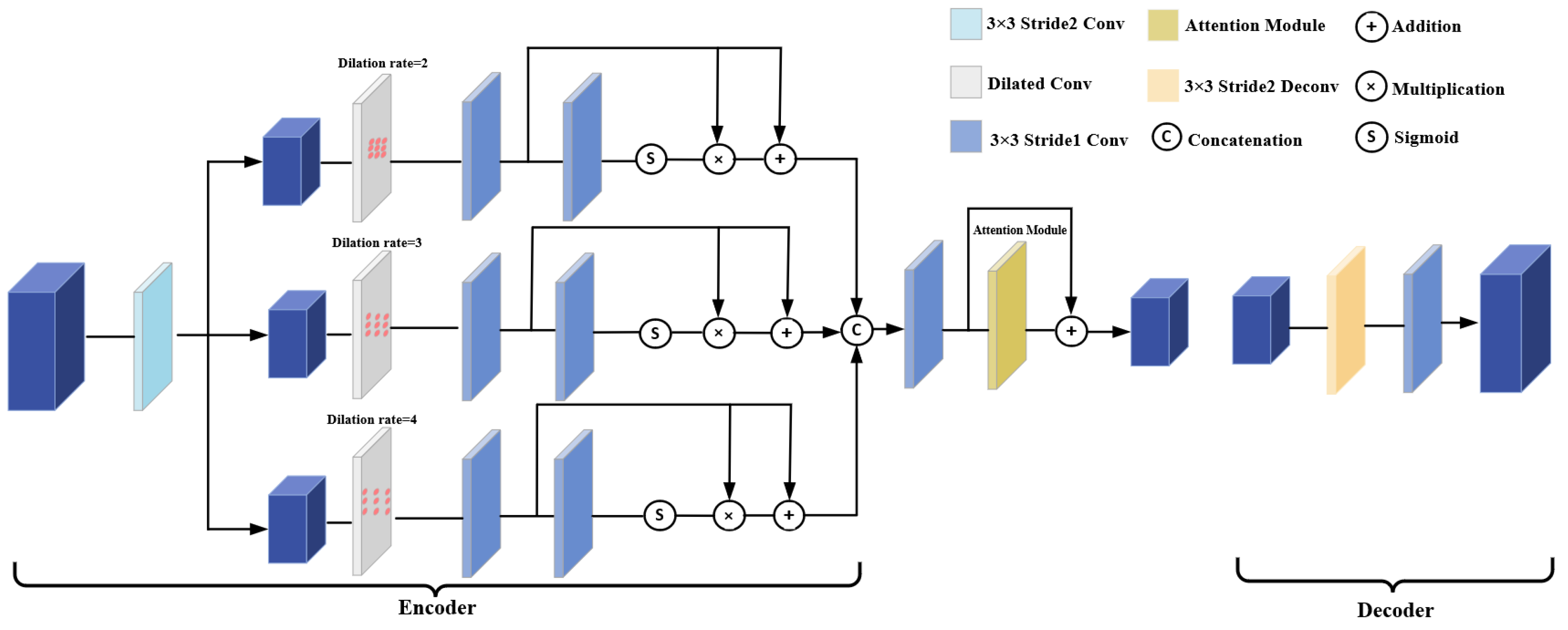
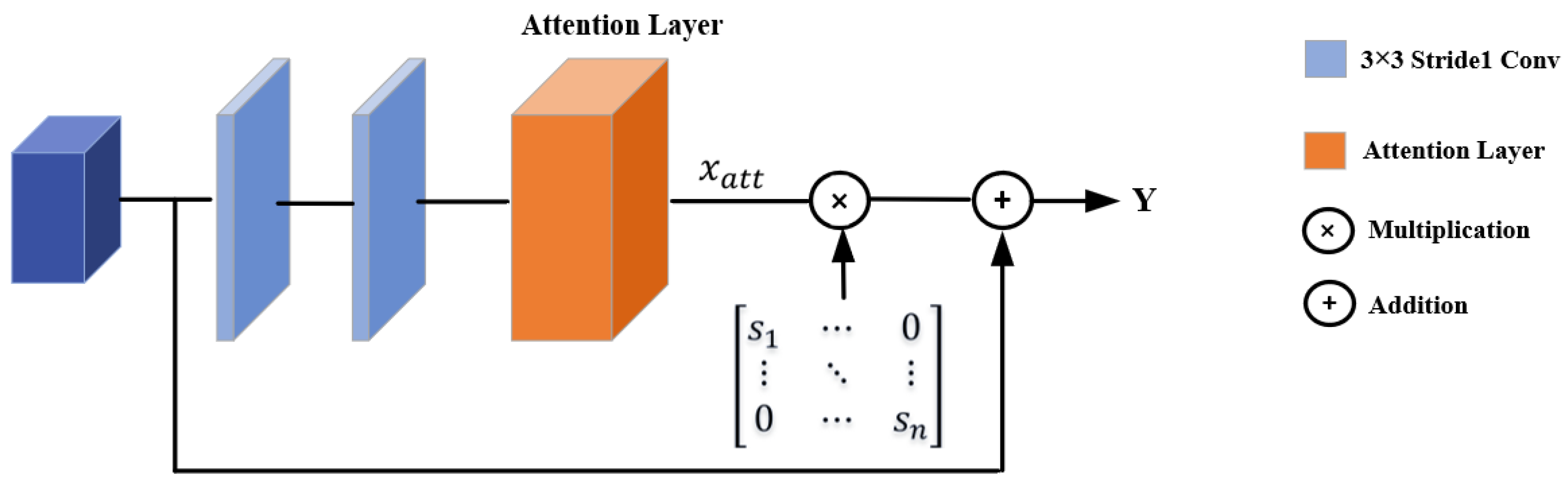
• We introduce a multi-scale feature extraction module based on triple dilated convolution and attention mechanism. This module increases the receptive field without adding model parameters, capturing dependencies between features to acquire global context information and enhance the representation of features in challenging regions;
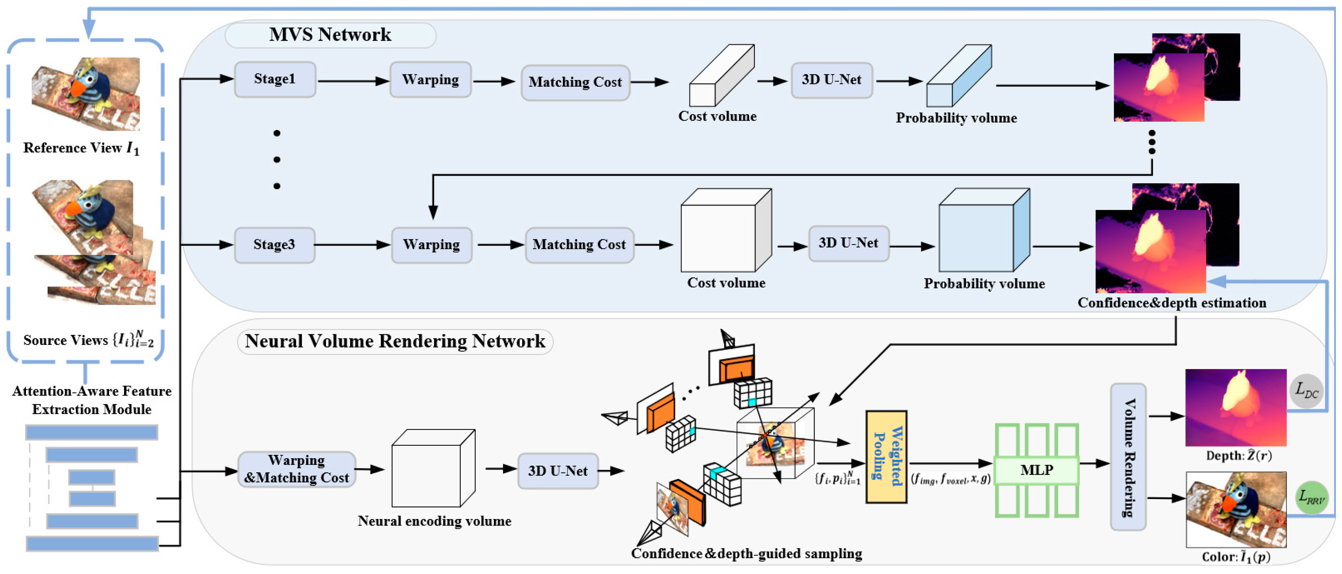
• We establish a neural volume rendering network using multi-view semantic features and neural encoding volume. The network is iteratively optimized through the rendering reference view loss, enabling the precise decoding of the geometric appearance information represented by the radiance field. We introduce the depth consistency loss to maintain geometric consistency between the MVS network and the neural volume rendering network, mitigating the impact of the flawed cost volume;
• Our approach demonstrates state-of-the-art results on the DTU dataset and the Tanks and Temples dataset.

The remaining structure of this paper is as follows. In Section 2, we present an overview of related work related to learning-based MVS networks and neural volume rendering. Subsequently, in Section 3, we delve into the various components of our proposed MVS network based on attention mechanism and neural volume rendering. Section 4 reports an extensive set of experimental results on the DTU dataset and the Tanks and Temples dataset, supplemented by ablation experiments to validate the effectiveness of the proposed modules. Finally, in Section 5, we offer the conclusion of the article.

2. Related Work

2.1. Learning-Based Multi-View Stereo

In light of the flourishing progress in deep learning technologies, a multitude of researchers have harnessed CNN to tackle MVS tasks. As a representative work, MVSNet [6] has established a deep learning-based MVS pipeline. This pipeline generates a 3D cost volume by integrating features from various perspectives through differentiable homography transformations. Subsequently, 3D CNN are employed to refine the cost volume to perform depth regression. Nonetheless, MVSNet consumes a substantial amount of memory, prompting subsequent efforts to seek more lightweight approaches. The study [16] has employed the recurrent architecture, which adjusts two-dimensional feature maps along the depth direction sequentially using Gated Recurrent Units (GRUs). This approach avoids the memory consumption associated with adjusting the entire cost volume at once, enabling high-resolution reconstructions. Another approach [17] estimates and refines depth maps in a coarse-to-fine manner. Initially, it predicts low-resolution depth maps with a large depth interval. As the depth range decreases, the algorithm iteratively increases the depth map resolution. This algorithm effectively reduces memory consumption caused by excessively large cost volumes. However, due to the limitations of CNN in capturing feature information in challenging regions, such as areas with weak textures and non-Lambertian surfaces, subsequent efforts have introduced attention mechanism into the MVS network to enhance feature representations of images. Works like [7] have incorporated self-attention mechanism at the feature extraction stage, enabling the network to focus more on crucial information and capture interdependencies between pixels. Nevertheless, there remains significant room for improvement in point cloud reconstruction, particularly in challenging areas. Due to the inherent advantage of capturing global contextual information using self-attention mechanism in Transformer models [18], subsequent works [19,20,21] have introduced it into MVS, enabling a comprehensive understanding of the global context within the MVS model to extract rich information from the environment. However, this often leads to increased computational time and memory consumption, especially in the reconstruction of high-resolution and large-scale scenes, incurring substantial computational costs.

2.2. Neural Volume Rendering Based on Multi-View Stereo

The Neural Radiance Field (NeRF) [9] represents scenes as continuous implicit functions of position and direction for high-quality view synthesis, achieving photorealistic rendering results at a pixel level. Subsequent works [15,22] have extended NeRF using MVS to support various other neural rendering tasks. MVSNeRF [15] utilizes cost volume constructed by MVS for geometric-aware scene inference, combining it with neural volume rendering for radiance field reconstruction, enabling high-quality view synthesis even with a limited number of images. RC-MVSNet [22], on the other hand, leverages a strongly generalized cost volume derived from MVS, combining it with neural volume rendering to reconstruct implicit scenes. It introduces a neural volume rendering-based reference view synthesis loss to optimize implicit scene information, alleviating photometric blur issues on non-Lambertian reflecting surfaces encountered by unsupervised learning MVS network. Our method leverages a strongly generalized cost volume and incorporates crucial 2D feature information from multiple views for neural volume rendering. In an end-to-end learning manner, it precisely conducts geometric inference for scene perception, mitigating the impact of flawed cost volumes constructed due to incorrect matches in challenging regions by the MVS network.

3. Methods

In this section, we elucidate the overall architecture of the proposed method, as illustrated in Figure 1. This architecture primarily comprises the MVS network and the neural volume rendering network. Specifically, in the feature extraction stage, we introduce the attention-aware feature extraction module. This module combines dilated convolution with attention mechanism to extract more comprehensive feature information. The MVS network progressively constructs a probability volume in a coarse-to-fine manner to estimate the depth maps and confidence maps. Subsequently, we design a novel neural volume rendering network.

The multi-layer perceptron (MLP) network uses multi-view 2D feature along with the 3D neural encoding volume containing geometric-aware information as the mapping condition. Additionally, we adopt a uniform sampling strategy guided by depth maps and confidence maps to focus the scene sampling on the estimated depth surface region. Finally, we apply the rendering reference view loss $L_{RRV}$ to precisely resolve the geometric shape of the scene from the radiance field. We also introduce the depth consistency loss $L_{DC}$ to ensure geometric consistency between the MVS network and the neural volume rendering network. It is noteworthy that the proposed network architecture functions as a universal framework for training the MVS network, making it applicable to any learning-based MVS network. The two networks provide mutual supervision and are simultaneously optimized.

3.1. Attention-Aware Feature Extraction Module

We propose the attention-aware feature extraction module. This module exhibits resemblances to a 2D U-Net, featuring elementary units that encompass both an encoder and a decoder, complete with skip connections. The encoder forms a network composed of dilated convolutional layers and an attention module, as depicted in Figure 2. In the encoder section, the features are initially subsampled using a convolutional layer with a stride of 2. Subsequently, dilated convolutional layers with 3 × 3 kernel are employed to expand the receptive field of the input features. To address potential information correlation issues associated with the use of dilated convolution, we adopt a strategy similar to that of [23], where feature maps are passed through a residual network structure with Sigmoid function after undergoing dilated convolutional layer with different dilation rate. To create the final feature map, the three fine-grained features are combined and run through a convolutional layer with an attention module. A convolutional layer and deconvolutional layer with 3 × 3 kernel make up the decoder. When provided with a reference image $I_1$ and source images ${\left\{I_i\right\}}_{i=2}^N$ at a resolution of $H\times W$ captured from different viewpoints, the attention-aware feature extraction module outputs three different scales of features, denoted as ${\left\{F_{i,k=1}\in R^{\frac{H}{4}\times \frac{W}{4}\times 32},F_{i,k=2}\in R^{\frac{H}{2}\times \frac{W}{2}\times 16},F_{i,k=3}\in R^{H\times W\times 8}\right\}}_{i=1}^N$, where $k$ represents the $k$-th stage.

Figure 3 provides a visual representation of the attention module’s architectural design. The features, which have undergone triple dilated convolution, are input into two convolutional layers with 3 × 3 kernel. Each of these layers goes through Group Normalization (GN) and a ReLU activation function. Subsequently, we incorporate a LayerScale-based local attention layer [24]. The operational details of this local attention layer are elucidated in Figure 4, illustrating the mapping of queries and a collection of key-value pairs to generate an output, with pixel outputs computed via Softmax operation.

$$y_{ij}={\displaystyle \sum _{a,b\in R}{\omega }_{ab}\left(q_{ij}^T\right(k_{ab}+r_{ab}\left)\right)v_{ab}}$$

(1)

In this equation, $q_{ij}=W_q{x}_{ij},k_{ab}=W_k{x}_{ab}$ and $v_{ab}=W_v{x}_{ab}$ represent the queries, keys, and values, respectively, with the matrices $W_n(n=q,k,v)$ composed of learnable parameters. Here, $R$ denotes a local region with a 3 × 3 input size. To address the issue of permutation equivariance resulting from the lack of encoded positional information, we introduce relative positional embeddings by incorporating learnable parameters into the keys, as described in [25]. The relative distance vector $r_{ab}$ is partitioned along the dimensions, with half of the dimension of the output channel allocated for encoding the row direction and the remaining half for encoding the column direction. Furthermore, the features $x_{att}$, produced by the attention layer, need to be multiplied by the learned diagonal matrix weights within the network.

$$Y=diag(s_1,\dots ,s_n)\times x_{att}+x$$

(2)

where $s_1$ to $s_n$ are learnable weights.

3.2. Cost Volume Construction

Subsequently, we perform adaptive depth hypothesis sampling using $J$ layers of depth hypothesis planes ${\left\{D_j\right\}}_{j=1}^J$. Based on these assumptions, we construct feature volumes ${\left\{V_i\right\}}_{i=1}^N$, which are constructed by differential warping 2D source views features to the reference view. Under the depth plane hypothesis $d$, the warping between a pixel $p$ in the reference view and its corresponding pixel $p_i^{\prime }$ in the $i$-th source view is defined as follows:

$$p_i^{\prime }=K_i[(R_i(d{K}^{-1}p)+t_i]$$

(3)

where $K_i$ and $K$ are the intrinsic matrix of the $i$-th source camera and the reference camera, respectively, $R_i$ and $t_i$ represent the rotation and translation between the two views.

Subsequently, we consolidate multiple feature volumes ${\left\{V_i\right\}}_{i=1}^N$ into a 3D cost volume $V$ using the variance-based aggregation strategy. Then, the cost volume is then regularized into a depth probability volume using a 3D U-Net. We determine the probability $P_j\left(p\right)$ on a specified depth plane $D_j\left(p\right)$ for the pixel $p$ in the reference view. Following this, we calculate the estimated depth value $\widehat{D}\left(p\right)$ for the pixel $p$ using the method outlined below:

$$\widehat{D}\left(p\right)={\displaystyle \sum _{j=1}^J{P}_j\left(p\right)D_j\left(p\right)}$$

(4)

3.3. Neural Volume Rendering Network

To further alleviate the issue of incorrect feature matching in MVS caused by significant differences in 3D location of features between adjacent views, we introduced a neural volume rendering network. This network is trained in a self-supervised manner to learn the scene geometry, providing the network with rich scene geometry information. This addition helps mitigate the impact of the flawed cost volume generated by incorrect matching issues in the MVS network.

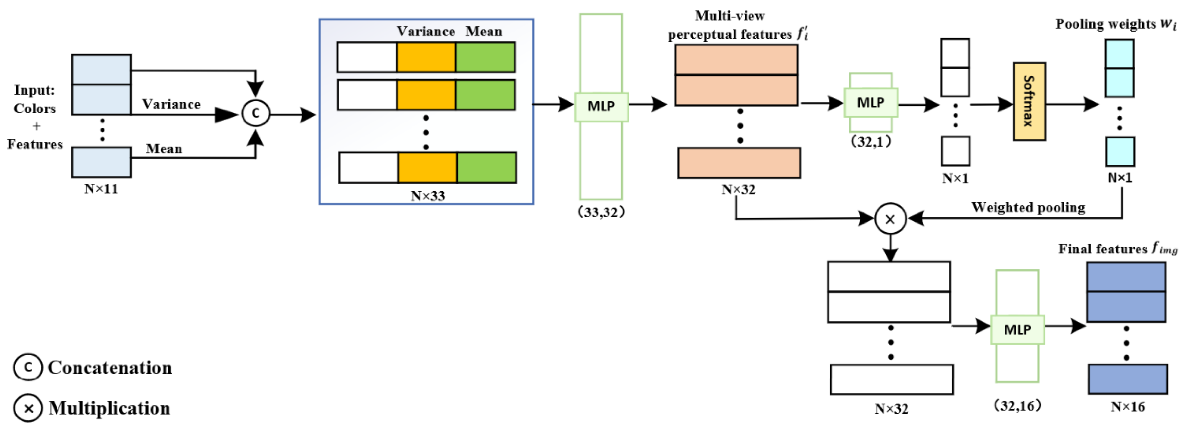
3.3.1. Scene Representation Based on Multi-View Features and Neural Encoding Volume

Our network extracts potential 2D feature vectors from the encoded contextual information of the source views. These multi-view 2D features provide additional semantic information about the scene, addressing 3D geometric ambiguity and enhancing the network’s ability to handle occlusion. Inspired by PixelNeRF [13], we project 3D points from arbitrary space into the input multi-view images. For N different views ${\left\{I_i\right\}}_{i=1}^N$, each having its corresponding extrinsic matrix $T_i=\left[R_i| t_i\right]$ concerning the target reference image and intrinsic matrix $K_i$. To acquire the color $c$ and volume density $\sigma$ of the 3D point, we begin by converting its 3D position $x$, and its reference view direction $g$, into the coordinate system of each view, leading to the 3D point $x_i=R_{i}x+t_i$. Subsequently, we project this point onto the corresponding pixel and feature maps and employ bilinear interpolation to sample its pixel $p_i$, and feature vector $f_i$:

$$f_i=F_i\left[K_i\left(R_{i}x+t_i\right)\right],g_i=R_{i}g$$

(5)

where $g_i$ represents the projection of the 3D point $x$’s reference view direction onto the respective observation directions of the multi-view images.

We utilize a weighted pooling operator, denoted as $\psi$, to aggregate the multi-view feature vectors, as illustrated in Figure 5. Initially, we combine the feature vector $f_i$ with the pixel information $p_i$ to create a two-dimensional feature vector. Subsequently, we compute the mean $\mu$ and variance $\nu$ of the two-dimensional feature vector to capture both local and global information. Then, the two-dimensional feature vector is concatenated with $\mu$ and $\nu$ fed into our specially designed lightweight MLP, extracting the multi-view perceptual features, denoted as $f_i^{\prime }$, and the pooling weights, denoted as $w_i$. Finally, by applying a Softmax operation to the weight vector, we perform a weighted pooling operation on the multi-view perceptual features, resulting in the final feature vector $f_{img}$:

$$f_{img}=\psi \left(f_1,\dots ,f_N\right)$$

(6)

Subsequently, following the same approach as in RC-MVSNet [22], we performed trilinear interpolation on the 3D neural encoding volume constructed using MVS, resulting in voxel-aligned three-dimensional feature voxel denoted as $f_{voxel}$. We then passed the weighted pooled final feature vector $f_{img}$ and the three-dimensional feature voxel $f_{voxel}$ through an MLP network to obtain RGB color $c$ and volume density $\sigma$ at 3D sampling points in the reference view direction.

$$[c,\sigma ]=\phi (f_{img},f_{voxel},{\gamma }_x(x),{\gamma }_g(g))$$

(7)

where, the position encoding function $\gamma$ aids in the network’s ability to recover high-frequency depth information.

3.3.2. Confidence and Depth-Guided Sampling for Volume Rendering

In the reference view $I_1$, each pixel $p$ corresponds to a ray defined in the world coordinate system. The 3D point associated with the pixel $p$ along this ray originating at a distance $e$ from the origin $o$ can be represented as $r_p=o+eg$. To render the color ${\tilde{I}}_1\left(p\right)$ at the pixel $p$, rays are uniformly sampled at $M$ discrete sample distances $e_m$ within the original NeRF near and far planes $[e_n,e_f]$. The radiance field $\phi$ at the 3D point is then queried:

$$e_m~\mu \left[e_n+\frac{m-1}{M}\left(e_f-e_n\right),t_n+\frac{m}{M}\left(e_f-e_n\right)\right]$$

(8)

Due to the uniform sampling probability within a sampling range in the original NeRF, the points may not be concentrated on the surface of the object, leading to a decrease in the quality of the rendered reference view. Therefore, for pixel $p$, we propose to sample candidate points under the guidance of the prior range defined by the depth estimation value $\widehat{D}\left(p\right)$ and its confidence from the MVS network.

We define the standard deviation $\widehat{S}$ as the degree of confidence for pixel $p$ with depth estimation value $\widehat{D}\left(p\right)$:

$$\widehat{S}\left(p\right)=\sqrt{{\displaystyle \sum _{j=1}^J{P}_j(p){(D_j(p)-\widehat{D}(p))}^2}}$$

(9)

The potential location of the object surface corresponding to each pixel should be confined within the interval defined by the depth estimation value $\widehat{D}\left(p\right)$ and the standard deviation $\widehat{S}\left(p\right)$, represented as $\widehat{U}\left(p\right)$:

$$\widehat{U}\left(p\right)=\left[\widehat{D}\left(p\right)-\widehat{S}\left(p\right),\widehat{D}\left(p\right)+\widehat{S}\left(p\right)\right]$$

(10)

Confidence and depth range $\widehat{U}\left(p\right)$ contain valuable signals to guide sampling along rays, thus, for rendering the color of a 3D point $x$ in the geometric scene, we replaced the coarse network used for hierarchical sampling in the original NeRF. We distribute half of the sampled points between the near plane $e_n$ and the far plane $e_f$. The second half of the sampled points are extracted within the range of the confidence and depth prior $\widehat{U}\left(p\right)$. This ensures both the network’s generalization capability and model convergence. Figure 6 presents a comparison between the two sampling methods.

Next, we render the predicted colors and volume density values ${\left\{\left(c_m,{\sigma }_m\right)\right\}}_{m=1}^M$ for each sampling point into the predicted reference pixel:

$${\tilde{I}}_1\left(p\right)={\displaystyle \sum _{m=1}^M{\alpha }_m}{c}_m$$

(11)

$${\alpha }_m=E_m\left(1-\exp \left(-{\sigma }_m{\delta }_m\right)\right)$$

(12)

$$E_m=\exp \left(-{\displaystyle \sum _{m^{\prime }=1}^m{\sigma }_{m^{\prime }}{\delta }_{m^{\prime }}}\right)$$

(13)

where $E_m$ represents the cumulative transmittance along the ray $e_m$, and ${\delta }_m=e_{m+1}-e_m$ is the distance between adjacent samples.

Our objective is to precisely deduce the depth value corresponding to the reference view from the radiance field. Therefore, we achieve the depth value for pixel $p$ by performing a density integral along the rays in the direction of the reference view.

$$\widehat{Z}\left(r\right)={\displaystyle \sum _{m=1}^M{\alpha }_m{e}_m}$$

(14)

3.4. Loss Function

Within the neural volume rendering network, following the methodology established in the original NeRF, we introduce the rendering reference view loss. This loss function utilizes mean squared error to quantify the disparity between the color of volume rendering along rays from the reference view and the color of the corresponding ground truth reference view. By optimizing the pixel values of the rendered reference view ${\tilde{I}}_1\left(p\right)$, we enhance the implicit geometric representation capability of the 3D scene.

$$L_{RRV}={\displaystyle \sum _p{‖{\tilde{I}}_1\left(p\right)-I_1\left(p\right)‖}_2^2}$$

(15)

To ensure geometric consistency between the two networks, we propose the depth consistency loss. This loss function employs $L_1$ loss to minimize the difference between the rendered depth and the estimated depth from the MVS network, while also minimizing the difference between the rendered depth and the ground truth depth.

$$L_{DC}={\displaystyle \sum _p{\displaystyle \sum _r\left[{\lambda }_{D{C}_1}{‖D_{GT}\left(p\right)-\widehat{Z}\left(r\right)‖}_{{}_1}+{\lambda }_{D{C}_2}{‖\widehat{D}\left(p\right)-\widehat{Z}\left(r\right)‖}_{{}_1}\right]}}$$

(16)

Within the MVS network, we utilize the $L_1$ loss as the training loss, quantifying the divergence between the ground truth depth and the estimated depth.

$$L_{MVS}={\displaystyle \sum _p{‖D_{GT}\left(p\right)-\widehat{D}\left(p\right)‖}_{{}_1}}$$

(17)

In the end, the overall training loss function for the end-to-end network is given by the following:

$$L= {\lambda }_{RRV}{L}_{RRV}+{\lambda }_{\mathrm{DC}}{L}_{DC}+{\lambda }_{MVS}{L}_{MVS}$$

(18)

4. Experiments

We comprehensively present the performance of our proposed method through a series of experiments. Additionally, we perform ablation experiments to validate the efficacy of our proposed attention-aware feature extraction module, loss functions, and the confidence and depth-guided sampling strategy.

4.1. Datasets

We conducted model training and evaluation using the DTU dataset [26] and the Tanks and Temples dataset [27]. The DTU dataset comprises 124 scenes captured from 49 distinct viewpoints, covering a range of 7 diverse lighting conditions, and collected using a robotic arm in indoor environments. We assess the reconstructed point cloud using three measurement criteria: Accuracy, Completeness, and Overall.

Accuracy represents the average distance between the reconstructed point cloud and the ground truth point cloud, calculated by the Formula (20). Completeness indicates the number of surfaces from the ground truth point cloud that are captured in the reconstructed point cloud within the same world coordinates, computed using Formula (22). Overall is the average of Accuracy and Completeness, calculated as per Formula (23).

$$di{s}_{re\to gr}=\underset{gr\in GR}{min}|re-gr|$$

(19)

$$Acc.= \frac{100}{\left|RE\right|}{\displaystyle \sum _{re\in RE}di{s}_{re\to gr}}$$

(20)

where $RE$ denotes the reconstructed point cloud, $GR$ represents the ground truth point cloud, and $di{s}_{re\to gr}$ signifies the shortest distance from a point in the reconstructed point cloud to the ground truth point cloud.

$$di{s}_{gr\to re}=\underset{re\in RE}{min}|gr-re|$$

(21)

$$Comp.= \frac{100}{\left|GR\right|}{\displaystyle \sum _{gr\in GR}di{s}_{gr\to re}}$$

(22)

where $di{s}_{gr\to re}$ represents the shortest distance from a point in the ground truth point cloud to the reconstructed point cloud.

$$Overall= \frac{Acc.+Comp.}{2}$$

(23)

The Tanks and Temples dataset, on the other hand, captures complicated real-world sceneries with 8 intermediate subsets and 6 advanced subsets.

We utilize the F-score as the evaluation metric for the Tanks and Temples dataset. The F-score takes into account the precision $PR$ and recall $RE$ of the reconstructed point cloud, with precision defined as in Equation (20) and recall as in Equation (22). The F-score is calculated according to the formula in Equation (24).

$$F-score= \frac{2PR\cdot RE}{PR+RE}$$

(24)

4.2. End-to-End Training Details

We fixed the number of input images at $N=4$ and resized the original images to a resolution of 512 × 640 pixels during the training phase. We divided the MVS network into three stages, with each stage taking input images at 1/16, 1/4, and 1 of the original resolution, respectively. We assumed the same number of plane sweep depths and depth intervals as [17]. Specifically, for the three stages, we assumed 48, 32, and 8 plane sweep depths and depth intervals of 4, 2, and 1, respectively. In the neural volume rendering network, we set the number of ray samples to 1024. We used the Adam optimizer with ${\lambda }_{D{C}_1}$ = 0.8, ${\lambda }_{D{C}_2}$ = 0.2, ${\lambda }_{RRV}$ = 1, ${\lambda }_{DC}$ = 0.01 and ${\lambda }_{MVS}$ = 1. The training process comprised 16 epochs, commencing with an initial learning rate of 0.0001. This learning rate was halved at the 10th, 12th, and 14th epoch. Our method was trained with a batch size of 2 using 2 Nvidia GTX 3090ti GPUs.

4.3. Experimental Results

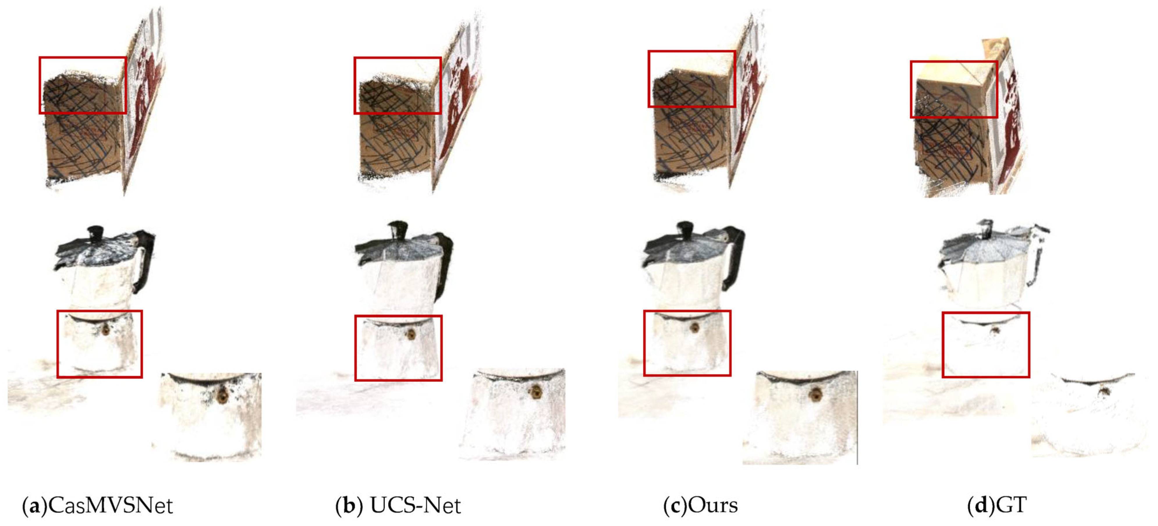
4.3.1. Results on DTU Dataset

Our model was assessed with 5 neighboring views ($N=5$) and input images at a resolution of 1152 × 864 pixels. We conducted a comparative analysis between our outcomes and those obtained from various traditional techniques as well as cutting-edge learning-based approaches. The quantitative evaluation results are presented in

Table 1. Quantitative results for the DTU dataset are presented. (lower scores indicate better performance). These results are categorized into traditional methods and learning-based methods. The other research results referenced in this study, other than our own, are taken from previously released research.

	Method	Acc. (mm)	Comp. (mm)	Overall (mm)
Traditional	Tola [30]	0.613	0.941	0.777
	Furu [2]	0.342	1.190	0.766
	Camp [1]	0.835	0.554	0.695
	Gipuma [3]	0.283	0.873	0.578
	Colmap [4]	0.400	0.644	0.532
Learning-based	MVSNet [6]	0.396	0.527	0.462
	CIDER [31]	0.417	0.437	0.427
	R-MVSNet [16]	0.383	0.452	0.417
	P-MVSNet [32]	0.406	0.434	0.420
	Point-MVSNet [33]	0.342	0.411	0.376
	Fast-MVSNet [34]	0.336	0.403	0.370
	PVA-MVSNet [35]	0.379	0.336	0.357
	CasMVSNet [17]	0.325	0.385	0.355
	UCS-Net [29]	0.338	0.349	0.344
	CVP-MVSNet [28]	0.296	0.406	0.351
	PatchmatchNet [36]	0.427	0.277	0.352
	EPP-MVSNet [37]	0.413	0.296	0.355
	AA-RMVSNet [38]	0.376	0.339	0.357
	Ours	0.363	0.296	0.329

. Our method excelled in terms of completeness, exhibiting a significant 27% improvement compared to CVP-MVSNet [28]. Moreover, our approach outperformed existing advanced methods in terms of overall reconstruction quality. In addition to quantitative analysis, Figure 7 provides visual qualitative results of the reconstructed point clouds. Our model generated more complete point clouds with finer texture details in challenging regions characterized by weak textures and lighting reflections compared to CasMVSNet [17] and UCS-Net [29].

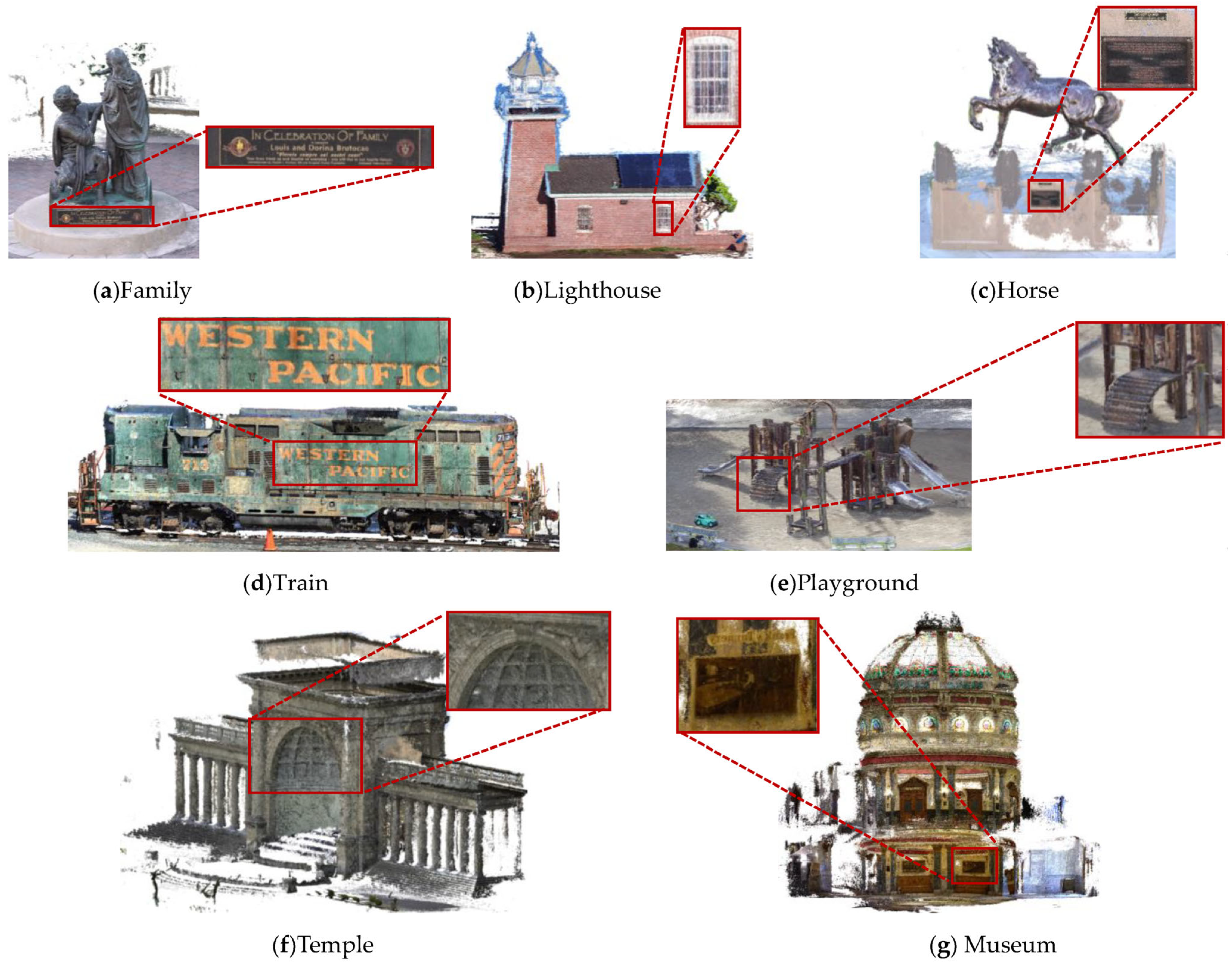
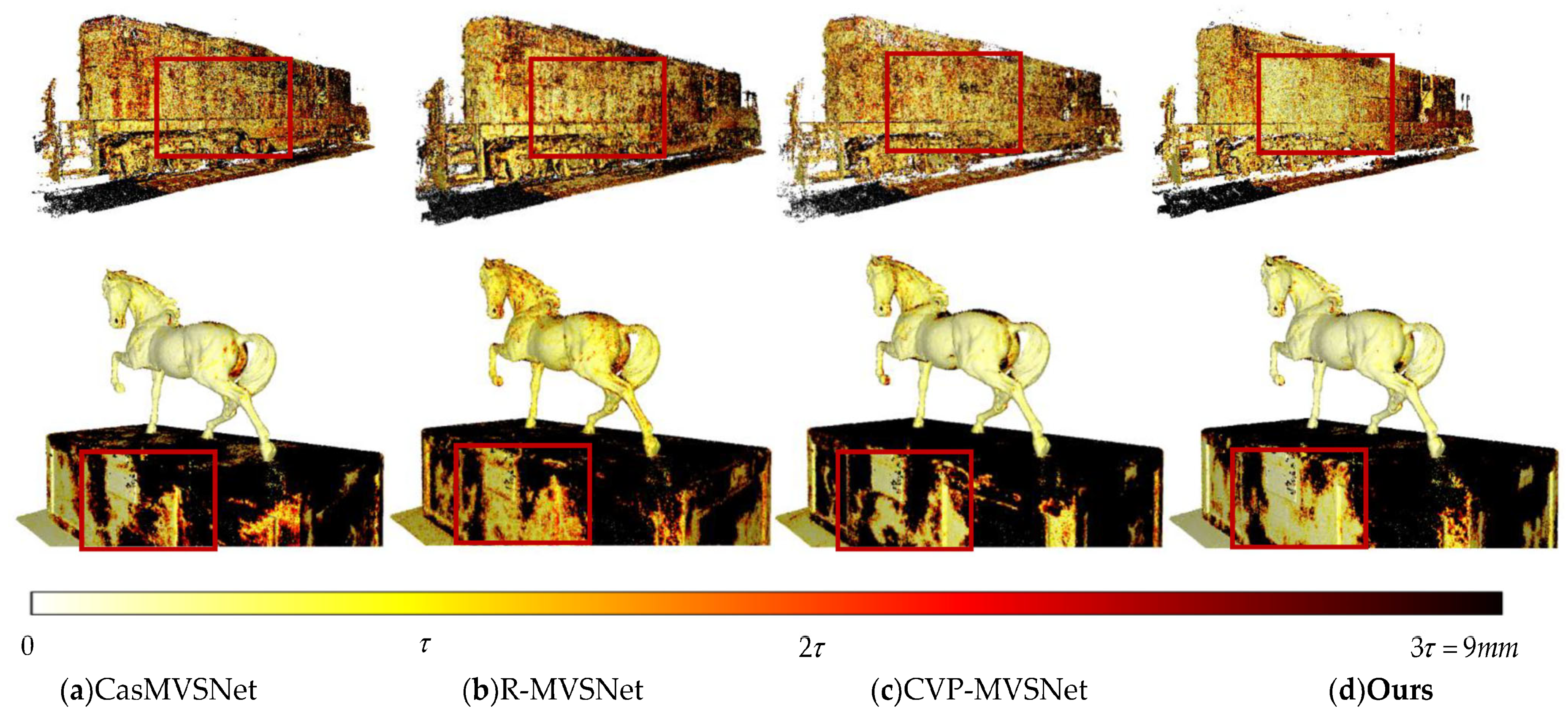
4.3.2. Results on Tanks and Temples Dataset

We conducted assessments using input images at a resolution of 1920 × 1080 and a neighboring view count set to $N=$ 5.

Table 2. The quantitative results of the F-score in the intermediate subset of the Tanks and Temples dataset are presented below (higher scores indicate better performance).

Method	Mean	Fam.	Fra.	Hor.	Lig.	M60.	Pan.	Pla.	Tra.
Point-MVSNet [33]	48.27	61.79	41.15	34.20	50.79	51.97	50.85	52.38	43.06
MVSNet [6]	43.48	55.99	28.55	25.07	50.79	53.96	50.86	47.90	34.69
Fast-MVSNet [34]	47.39	65.18	39.59	34.98	47.81	49.16	46.20	53.27	42.91
UCS-Net [29]	54.83	76.09	53.16	43.03	54.00	55.60	51.49	57.38	47.89
CIDER [31]	46.76	56.79	32.39	29.89	54.67	53.46	53.51	50.48	42.85
R-MVSNet [16]	48.40	69.96	46.65	32.59	42.95	51.88	48.80	52.00	42.38
P-MVSNet [32]	55.62	70.04	44.64	40.22	65.20	55.08	55.17	60.37	54.29
PatchmatchNet [36]	53.15	66.99	52.64	43.24	54.87	52.87	49.54	54.21	50.81
PVA-MVSNet [35]	54.46	69.36	46.80	46.01	55.74	57.23	54.75	56.70	49.06
CVP-MVSNet [28]	54.03	76.50	47.74	36.34	55.12	57.28	54.28	57.43	47.54
MVSTR [20]	56.93	76.92	59.82	50.16	56.73	56.53	51.22	56.58	47.48
CasMVSNet [17]	56.42	76.36	58.45	46.20	55.53	56.11	54.02	58.17	46.56
Ours	58.00	76.65	56.19	50.20	55.69	60.69	57.34	53.86	53.43

presents quantitative results for the intermediate subset. Our method demonstrates superior performance across most intermediate subsets, underscoring its effectiveness and generalization capability. Figure 8 offers illustrative qualitative visualizations of the 3D point clouds reconstructed, highlighting the robust reconstruction capabilities of our algorithm. Figure 9 showcases qualitative results for the “Train” and “Horse” scenes within the intermediate subset. Our method excels in producing more precise and comprehensive points, particularly in regions with low-texture attributes or non-Lambertian surfaces. In the more complex advanced subsets, as delineated in

Table 3. We present the quantitative results of the F-score within the advanced subset of the Tanks and Temples dataset, with higher scores indicative of superior performance.

Method	Mean	Aud.	Bal.	Court.	Mus.	Pal.	Tem.
R-MVSNet [16]	24.91	12.55	29.09	25.06	38.68	19.14	24.96
CIDER [31]	23.12	12.77	24.94	25.01	33.64	19.18	23.15
PatchmatchNet [36]	32.31	23.69	37.73	30.04	41.80	28.31	32.29
CasMVSNet [17]	31.12	19.81	38.46	29.10	43.87	27.36	28.11
Ours	31.66	22.75	38.77	28.55	39.46	30.53	29.91

, our approach performs better than previous advanced learning-based approaches in the scene “Ballroom” and scene “Palace”.

4.4. Ablation Study

We conducted four comparative experiments on the DTU evaluation dataset. We investigated the impact of different loss functions and the attention-aware feature extraction module on the reconstruction results. Additionally, we examined the impact of varying dilation rates in the attention-aware feature extraction module on the reconstruction results. We also assessed the influence of confidence and depth-guided sampling strategy under different view counts on the reconstruction results. Finally, we evaluated the network’s performance when varying the number of rays used for sampling.

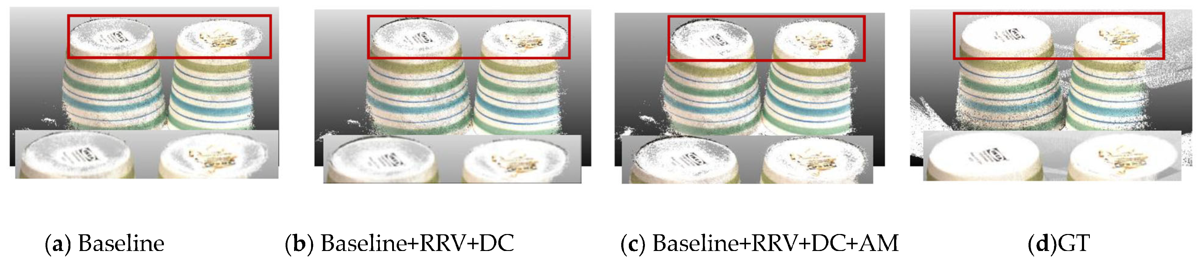
4.4.1. Influence of Attention-Aware Feature Extraction Module and Different Loss Functions

We have discussed the impact of the attention-aware feature extraction module and different loss functions on the final reconstruction of point clouds and the associated effects on model parameters, inference time, and memory usage during testing, building upon the baseline model CasMVSNet. The outcomes are displayed in

Table 4. Ablation study of attention-aware feature extraction module and different loss functions. The baseline represents CasMVSNet. AM represents the attention-aware feature extraction module. RRV represents rendering reference view loss. DC represents depth consistency loss.

Method	Acc. (mm)	Comp. (mm)	Overall (mm)	Test Param.	Test Time (s)	Test Memory (GB)
Baseline	0.325	0.385	0.355	934,304	0.49	5.3
Baseline + AM	0.357	0.324	0.340	964,943	0.528	5.4
Baseline + RRV	0.359	0.313	0.336	934,304	0.49	5.3
Baseline + RRV + DC	0.364	0.305	0.334	934,304	0.49	5.3
Baseline + RRV + DC + AM	0.363	0.296	0.329	964,943	0.528	5.4

, clearly illustrating that the attention-aware feature extraction module along with the two loss functions significantly enhances the integrity of the point cloud reconstruction. When these components are combined with the baseline CasMVSNet model, the improvement in point cloud reconstruction is most prominent in terms of integrity assessment, while maintaining a high overall evaluation level. Our proposed model, during the evaluation process on the test dataset, bypasses the neural volume rendering network. Instead, it utilizes the MVS network to estimate depth maps based on the learned feature weights. As a result, a minor increase in the number of parameters, inference time, and memory usage over the baseline model is introduced to enhance the completeness and overall quality of the reconstructed point clouds. We also visualize the influence of these components on the reconstruction results, as shown in Figure 10. By adding the neural volume rendering network and incorporating rendering reference view loss and depth consistency loss to the baseline CasMVSNet, the neural volume rendering network learns additional scene geometry information beyond the cost volume representing scene geometry. This leads to an enhancement in the completeness of the reconstructed point cloud. Additionally, the inclusion of the attention-aware feature extraction module extracts rich feature information to mitigate feature-matching errors, resulting in improved reconstruction results for point clouds in regions with weak texture and non-Lambertian surfaces.

4.4.2. Impact of Different Dilation Rates in the Attention-Aware Feature Extraction Module

Table 5. Different dilation rates of the dilated convolutions in the attention-aware feature extraction module on the reconstruction results.

Dilation Rate	Acc. (mm)	Comp. (mm)	Overall (mm)
(1, 2, 3)	0.358	0.306	0.332
(2, 3, 4)	0.363	0.296	0.329
(2, 3, 5)	0.365	0.313	0.339
(1, 3, 5)	0.370	0.312	0.341
(3, 4, 5)	0.379	0.329	0.354

presents the influence of different dilation rates in the attention-aware feature extraction module on the reconstruction results. When the dilation rates of the three dilated convolutions are set to 2, 3, and 4, the overall quality of point cloud reconstruction is the best. However, as the dilation rate increase, the continuity of extracted feature information decreases, resulting in reduced information coherence, and consequently, the overall quality of point cloud reconstruction by the network deteriorates.

4.4.3. Effect of Confidence and Depth-guided Sampling Strategy under Different Numbers of Input Views

Table 6. Ablation study of confidence and depth-guided sampling strategy under different view counts. CDG represents the confidence and depth-guided sampling strategy.

Nviews	CDG	Acc. (mm)	Comp. (mm)	Overall (mm)
3		0.377	0.325	0.351
3	✓	0.367	0.315	0.341
4		0.374	0.299	0.336
4	✓	0.363	0.296	0.329
5		0.379	0.305	0.342
5	✓	0.370	0.302	0.336

demonstrates the impact of sampling within the confidence and depth prior range on the reconstruction results under varying numbers of views. The point cloud reconstruction achieves the best overall quality when the number of views is set to 4. Therefore, we adopted this view count for other ablation analyses. Furthermore, the confidence and depth-guided sampling strategy concentrates on collecting points near the object’s surface. This allows the network to accurately construct the geometric shape of the neural radiance field, thereby mitigating the impact of the flawed cost volume on the network. Consequently, the point cloud reconstruction exhibits an overall improvement in performance.

4.4.4. Performance of Sampling with Varying Numbers of Rays

During volume rendering, we quantitatively assessed the impact of varying the number of sampled rays on point cloud reconstruction results. As shown in

Table 7. The quantitative performance with different quantities of ray sampling.

Num_Rays	Acc. (mm)	Comp. (mm)	Overall (mm)
256	0.371	0.304	0.337
1024	0.363	0.296	0.329
4096	0.369	0.300	0.334
8192	0.363	0.297	0.330

, we conducted experiments with four different sampling quantities. The point cloud reconstruction achieved the best accuracy and completeness evaluation results when the number of sampled rays reached 1024.

5. Conclusions

In this research, we introduce an attention-aware feature extraction network to capture inter-pixel dependencies and adequately extract semantic information from the original views. Furthermore, we establish a novel neural volume rendering network based on multi-view semantic features and neural encoding volume, utilizing rendering reference view loss to reconstruct the 3D scene geometry. Additionally, we introduce depth consistency loss to maintain the consistency of scene geometry, alleviating the impact of incorrect matching in regions with weak texture or non-Lambertian surfaces. Extensive experimentation on both the DTU and Tanks and Temples datasets showcases the superior performance of our network compared to previous state-of-the-art approaches. Comprehensive ablation studies validate the effectiveness of the individual modules introduced.

References

1. Campbell, N.D.; Vogiatzis, G.; Hernández, C.; Cipolla, R. Using multiple hypotheses to improve depth-maps for multi-view stereo. In Proceedings of the European Conference on Computer (ECCV), Marseille, France, 12–18 October 2008; pp. 766–779. [Google Scholar]
2. Ponce, J.; Furukawa, Y. Accurate, Dense, and Robust Multiview Stereopsis. IEEE Trans. Pattern Anal. Mach. Intell. 2010, 32, 1362–1376. [Google Scholar] [CrossRef]
3. Galliani, S.; Lasinger, K.; Schindler, K. Massively parallel multiview stereopsis by surface normal diffusion. In Proceedings of the IEEE International Conference on Computer Vision (ICCV), Santiago, Chile, 7–13 December 2015; pp. 873–881. [Google Scholar]
4. Schönberger, J.L.; Zheng, E.; Frahm, J.-M.; Pollefeys, M. Pixelwise view selection for unstructured multi-view stereo. In Proceedings of the European Conference on Computer (ECCV), Amsterdam, The Netherlands, 11–14 October 2016; pp. 501–518. [Google Scholar]
5. Xu, Q.; Tao, W. Multi-scale geometric consistency guided multi-view stereo. In Proceedings of the IEEE/CVF Conference on Computer Vision and Pattern Recognition (CVPR), Long Beach, CA, USA, 16–20 June 2019; pp. 5483–5492. [Google Scholar]
6. Yao, Y.; Luo, Z.; Li, S.; Fang, T.; Quan, L. MVSNet: Depth inference for unstructured multi-view stereo. In Proceedings of the European Conference on Computer Vision (ECCV), Munich, Germany, 8–14 September 2018; pp. 767–783. [Google Scholar]
7. Yu, A.; Guo, W.; Liu, B.; Chen, X.; Wang, X.; Cao, X.; Jiang, B.J.I.J.o.P.; Sensing, R. Attention aware cost volume pyramid based multi-view stereo network for 3d reconstruction. ISPRS J. Photogramm. Remote Sens. 2021, 175, 448–460. [Google Scholar] [CrossRef]
8. Li, J.; Bai, Z.; Cheng, W.; Liu, H. Feature Pyramid Multi-View Stereo Network Based on Self-Attention Mechanism. In Proceedings of the 2022 5th International Conference on Image and Graphics Processing, Beijing, China, 7–9 January 2022; pp. 226–233. [Google Scholar]
9. Mildenhall, B.; Srinivasan, P.P.; Tancik, M.; Barron, J.T.; Ramamoorthi, R.; Ng, R. NeRF: Representing scenes as neural radiance fields for view synthesis. Commun. ACM 2020, 65, 99–106. [Google Scholar] [CrossRef]
10. Xu, Q.; Xu, Z.; Philip, J.; Bi, S.; Shu, Z.; Sunkavalli, K.; Neumann, U. Point-NeRF: Point-based Neural Radiance Fields. In Proceedings of the 2022 IEEE/CVF Conference on Computer Vision and Pattern Recognition (CVPR), New Orleans, LA, USA, 19–24 June 2022; pp. 5428–5438. [Google Scholar]
11. Yang, J.; Pavone, M.; Wang, Y. FreeNeRF: Improving Few-shot Neural Rendering with Free Frequency Regularization. In Proceedings of the IEEE/CVF Conference on Computer Vision and Pattern Recognition (CVPR), Oxford, UK, 15–17 September 2023; pp. 8254–8263. [Google Scholar]
12. Wang, Q.; Wang, Z.; Genova, K.; Srinivasan, P.; Zhou, H.; Barron, J.T.; Martin-Brualla, R.; Snavely, N.; Funkhouser, T. IBRNet: Learning Multi-View Image-Based Rendering. In Proceedings of the 2021 IEEE/CVF Conference on Computer Vision and Pattern Recognition (CVPR), Nashville, TN, USA, 19–25 June 2021; pp. 4688–4697. [Google Scholar]
13. Yu, A.; Ye, V.; Tancik, M.; Kanazawa, A. pixelNeRF: Neural radiance fields from one or few images. In Proceedings of the IEEE/CVF Conference on Computer Vision and Pattern Recognition (CVPR), Nashville, TN, USA, 19–25 June 2021; pp. 4578–4587. [Google Scholar]
14. Garbin, S.J.; Kowalski, M.; Johnson, M.; Shotton, J.; Valentin, J. FastNeRF: High-Fidelity Neural Rendering at 200FPS. In Proceedings of the IEEE/CVF International Conference on Computer Vision (ICCV), Montreal, QC, Canada, 10–17 October 2021; pp. 14326–14335. [Google Scholar]
15. Chen, A.; Xu, Z.; Zhao, F.; Zhang, X.; Xiang, F.; Yu, J.; Su, H. MVSNeRF: Fast generalizable radiance field reconstruction from multi-view stereo. In Proceedings of the IEEE/CVF International Conference on Computer Vision (CVPR), Nashville, TN, USA, 19–25 June 2021; pp. 14124–14133. [Google Scholar]
16. Yao, Y.; Luo, Z.; Li, S.; Shen, T.; Fang, T.; Quan, L. Recurrent MVSNet for High-Resolution Multi-View Stereo Depth Inference. In Proceedings of the IEEE/CVF Conference on Computer Vision and Pattern Recognition (CVPR), Long Beach, CA, USA, 16–20 June 2019; pp. 5520–5529. [Google Scholar]
17. Gu, X.; Fan, Z.; Zhu, S.; Dai, Z.; Tan, F.; Tan, P. Cascade cost volume for high-resolution multi-view stereo and stereo matching. In Proceedings of the IEEE/CVF Conference on Computer Vision and Pattern Recognition (CVPR), Seattle, WA, USA, 14–19 June 2020; pp. 2495–2504. [Google Scholar]
18. Vaswani, A.; Shazeer, N.; Parmar, N.; Uszkoreit, J.; Jones, L.; Gomez, A.N.; Kaiser, Ł.; Polosukhin, I. Attention is all you need. Adv. Neural Inf. Process. Syst. 2017, 30, 5998–6008. [Google Scholar]
19. Ding, Y.; Yuan, W.; Zhu, Q.; Zhang, H.; Liu, X.; Wang, Y.; Liu, X. TransMVSNet: Global Context-aware Multi-view Stereo Network with Transformers. In Proceedings of the IEEE/CVF Conference on Computer Vision and Pattern Recognition (CVPR), New Orleans, LA, USA, 19–24 June 2022; pp. 8575–8584. [Google Scholar]
20. Zhu, J.; Peng, B.; Li, W.; Shen, H.; Zhang, Z.; Lei, J. Multi-View Stereo with Transformer. arXiv 2021, arXiv:2112.00336. [Google Scholar]
21. Wang, X.; Zhu, Z.; Huang, G.; Qin, F.; Ye, Y.; He, Y.; Chi, X.; Wang, X. MVSTER: Epipolar transformer for efficient multi-view stereo. In Proceedings of the European Conference on Computer Vision (ECCV), Tel-Aviv, Israel, 23–27 October 2022; pp. 573–591. [Google Scholar]
22. Chang, D.; Božič, A.; Zhang, T.; Yan, Q.; Chen, Y.; Süsstrunk, S.; Nießner, M. RC-MVSNet: Unsupervised Multi-View Stereo with Neural Rendering. In Proceedings of the European Conference on Computer (ECCV), Tel-Aviv, Israel, 23–27 October 2022; pp. 665–680. [Google Scholar]
23. Lin, L.; Zhang, Y.; Wang, Z.; Zhang, L.; Liu, X.; Wang, Q. A-SATMVSNet: An attention-aware multi-view stereo matching network based on satellite imagery. Front. Earth Sci. 2023, 11, 1108403. [Google Scholar] [CrossRef]
24. Touvron, H.; Cord, M.; Sablayrolles, A.; Synnaeve, G.; Jégou, H. Going deeper with Image Transformers. arXiv 2021, arXiv:2103.17239. [Google Scholar]
25. Shaw, P.; Uszkoreit, J.; Vaswani, A. Self-attention with relative position representations. arXiv 2018, arXiv:1803.02155. [Google Scholar]
26. Aanæs, H.; Jensen, R.R.; Vogiatzis, G.; Tola, E.; Dahl, A.B. Large-scale data for multiple-view stereopsis. Int. J. Comput. Vis. 2016, 120, 153–168. [Google Scholar] [CrossRef]
27. Knapitsch, A.; Park, J.; Zhou, Q.-Y.; Koltun, V. Tanks and temples: Benchmarking large-scale scene reconstruction. ACM Trans. Graph. 2017, 36, 1–13. [Google Scholar] [CrossRef]
28. Yang, J.; Mao, W.; Alvarez, J.M.; Liu, M. Cost Volume Pyramid Based Depth Inference for Multi-View Stereo. In Proceedings of the IEEE/CVF Conference on Computer Vision and Pattern Recognition (CVPR), Seattle, WA, USA, 14–19 June 2020; pp. 4876–4885. [Google Scholar]
29. Cheng, S.; Xu, Z.; Zhu, S.; Li, Z.; Li, L.E.; Ramamoorthi, R.; Su, H. Deep Stereo Using Adaptive Thin Volume Representation With Uncertainty Awareness. In Proceedings of the IEEE/CVF Conference on Computer Vision and Pattern Recognition (CVPR), Seattle, WA, USA, 14–19 June 2020; pp. 2521–2531. [Google Scholar]
30. Tola, E.; Strecha, C.; Fua, P. Efficient large-scale multi-view stereo for ultra high-resolution image sets. Mach. Vis. Appl. 2012, 23, 903–920. [Google Scholar] [CrossRef]
31. Xu, Q.; Tao, W. Learning inverse depth regression for multi-view stereo with correlation cost volume. In Proceedings of the AAAI Conference on Artificial Intelligence, New York, NY, USA, 7–12 February 2020; pp. 12508–12515. [Google Scholar]
32. Luo, K.; Guan, T.; Ju, L.; Huang, H.; Luo, Y. P-MVSNet: Learning Patch-Wise Matching Confidence Aggregation for Multi-View Stereo. In Proceedings of the IEEE/CVF International Conference on Computer Vision (ICCV), Seoul, Republic of Korea, 27 October–2 November 2019; pp. 10451–10460. [Google Scholar]
33. Chen, R.; Han, S.; Xu, J.; Su, H. Point-Based Multi-View Stereo Network. In Proceedings of the IEEE/CVF International Conference on Computer Vision (ICCV), Seoul, Republic of Korea, 27 October–2 November 2019; pp. 1538–1547. [Google Scholar]
34. Yu, Z.; Gao, S. Fast-MVSNet: Sparse-to-Dense Multi-View Stereo With Learned Propagation and Gauss-Newton Refinement. In Proceedings of the IEEE/CVF Conference on Computer Vision and Pattern Recognition (CVPR), Seattle, WA, USA, 14–19 June 2020; pp. 1946–1955. [Google Scholar]
35. Yi, H.; Wei, Z.; Ding, M.; Zhang, R.; Chen, Y.; Wang, G.; Tai, Y.-W. Pyramid multi-view stereo net with self-adaptive view aggregation. In Proceedings of the European Conference on Computer (ECCV), Glasgow, UK, 23–28 August 2020; pp. 766–782. [Google Scholar]
36. Wang, F.; Galliani, S.; Vogel, C.; Speciale, P.; Pollefeys, M. Patchmatchnet: Learned multi-view patchmatch stereo. In Proceedings of the IEEE/CVF Conference on Computer Vision and Pattern Recognition (CVPR), Nashville, TN, USA, 19–25 June 2021; pp. 14194–14203. [Google Scholar]
37. Ma, X.; Gong, Y.; Wang, Q.; Huang, J.; Chen, L.; Yu, F. EPP-MVSNet: Epipolar-assembling based Depth Prediction for Multi-view Stereo. In Proceedings of the IEEE/CVF International Conference on Computer Vision (ICCV), Montreal, QC, Canada, 10–17 October 2021; pp. 5712–5720. [Google Scholar]
38. Wei, Z.; Zhu, Q.; Min, C.; Chen, Y.; Wang, G. AA-RMVSNet: Adaptive Aggregation Recurrent Multi-view Stereo Network. In Proceedings of the IEEE/CVF International Conference on Computer Vision (ICCV), Montreal, QC, Canada, 10–17 October 2021; pp. 6167–6176. [Google Scholar]
Figure 1. Illustration of the proposed approach. Our network consists of the MVS network and the neural volume rendering network.
Electronics 12 04603 g001
Figure 2. The design of the feature extraction module we propose.
Electronics 12 04603 g002
Figure 3. The architecture of the attention module. This module is a residual structure composed of a mixture of convolutional layers and a local attention layer.
Electronics 12 04603 g003
Figure 4. The architecture of the local attention layer.
Electronics 12 04603 g004
Figure 5. Weighted pooling operation. Here, N represents the number of input views. The notation below the MLP denotes the dimensions of input and output variables in the linear layer, respectively.
Electronics 12 04603 g005
Figure 6. Comparison of two sampling methods. In contrast to the uniform sampling employed in the original NeRF, the sampling method within confidence and depth prior range concentrates the samples more on the surface of the object.
Electronics 12 04603 g006
Figure 7. On the DTU dataset scan 13 and scan 77, we compare the reconstruction results with CasMVSNet, UCS-Net, and ground truth.
Electronics 12 04603 g007
Figure 8. Visualization of 3D point clouds of (a) the scene “Family”, (b) the scene “Lighthouse”, (c) the scene “Horse”, (d) the scene “Train”, (e) the scene “Playground”, (f) the scene “Temple”, and (g) the scene “Museum” on the intermediate and advanced subsets of the Tanks and Temples dataset.
Electronics 12 04603 g008
Figure 9. The precision results of the “Train” ( τ = 5   mm ) and the recall results of the “Horse” ( τ = 3   mm ) scenes reconstructed on the Tanks and Temples dataset are compared with the CasMVSNet, R-MVSNet, and CVP-MVSNet. Here, τ represents the official distance threshold, and darker regions indicate higher errors relative to τ .
Electronics 12 04603 g009
Figure 10. Qualitative results of scan 48 on the DTU dataset using the attention-aware feature extraction module and various loss functions.
Electronics 12 04603 g010