Article

RCA-GAN: An Improved Image Denoising Algorithm Based on Generative Adversarial Networks

1
Shijiazhuang Campus, Army Engineering University of PLA, Shijiazhuang 050003, China
2
Hebei University of Science and Technology, Shijiazhuang 050018, China
*
Author to whom correspondence should be addressed.
Electronics 2023, 12(22), 4595; https://doi.org/10.3390/electronics12224595
Submission received: 9 October 2023 / Revised: 26 October 2023 / Accepted: 3 November 2023 / Published: 10 November 2023
(This article belongs to the Special Issue Application of Machine Learning in Graphics and Images)

Abstract

:
Image denoising, as an essential component of image pre-processing, effectively reduces noise interference to enhance image quality, a factor of considerable research importance. Traditional denoising methods often lead to the blurring of image details and a lack of realism at the image edges. To deal with these issues, we propose an image denoising algorithm named Residual structure and Cooperative Attention mechanism based on Generative Adversarial Networks (RCA-GAN). This algorithm proficiently reduces noise while focusing on preserving image texture details. To maximize feature extraction, this model first employs residual learning within a portion of the generator’s backbone, conducting extensive multi-dimensional feature extraction to preserve a greater amount of image details. Secondly, it introduces a simple yet efficient cooperative attention module to enhance the representation capacity of edge and texture features, further enhancing the preservation of intricate image details. Finally, this paper constructs a novel loss function—the Multimodal Loss Function—for the network training process. The experimental results were evaluated using Peak Signal-to-Noise Ratio (PSNR) and Structural Similarity (SSIM) as evaluation metrics. The experimental results demonstrate that the proposed RCA-GAN image denoising algorithm has increased the average PSNR from 24.71 dB to 33.76 dB, achieving a 36.6% improvement. Additionally, the average SSIM value has risen from 0.8451 to 0.9503, indicating a 12.4% enhancement. It achieves superior visual outcomes, showcasing the ability to preserve image texture details to a greater extent and excel in edge preservation and noise suppression.

1. Introduction

Due to the inevitable noise during the image acquisition and transmission process, image quality frequently experiences degradation [1], impacting the reliability of subsequent image-related tasks across various fields [2]. Therefore, the need for achieving adaptive image enhancement is increasingly pressing. Image denoising, a classical technique in computer vision, aims to restore noise-free images from noisy counterparts, ensuring effective subsequent processing of high-quality images [3,4,5]. Hence, the pursuit of more practical image denoising methods to enhance image quality remains a focal point in the realm of image processing [6].
There are mainly traditional denoising methods and denoising methodologies rooted in deep learning techniques [7,8,9]. The traditional denoising methods include spatial domain filtering [10,11] and transform domain filtering [12]. Spatial domain filtering employs convolution techniques with image signals and filtering templates to complete the filtering process [13], including median filtering [14,15], mean filtering [16,17], and more. Transform domain filtering involves taking a noisy image and filtering it in the transform domain to obtain a denoised image. This process includes methods such as wavelet transform domain [18,19] and Fourier transform domain [20]. The Block-Matching and 3D filtering (BM3D) [21] method utilizes self-similar patches to attain superior outcomes with respect to both image fidelity and visual quality. While these methods are effective in noise suppression, the quality of the denoised images often falls short, and the feature extraction process they entail is laborious, time-consuming, and computationally intensive. This makes them less suitable for handling real noise characterized by intricate distributions.
In contrast to conventional image denoising algorithms, deep learning-based image denoising algorithms are data-oriented, capable of achieving higher performance metrics in fixed-mode image denoising, and enhancing image quality to some extent. Burger et al. [22] introduced the Multi-Layer Perceptron (MLP) algorithm for image denoising, which iteratively learns by constraining the difference between network outputs and actual images using the L2 loss function. Zhang et al. [23] introduced the Denoising Convolutional Neural Network (DnCNN) image denoising algorithm, which incorporates residual learning [24] and batch normalization to broaden the scope of denoising tasks, encompassing universal image denoising and enhancing denoising performance. In the literature [25], a two-channel residual convolutional network was proposed to address underwater image denoising. This approach utilizes both local residual and global sparse blocks for feature extraction and employs feature processing blocks to achieve feature fusion, ultimately leading to an improvement in image quality. To enhance the denoising capabilities of traditional Convolutional Neural Network (CNN), Lan et al. [26] introduced the deep residual convolutional neural network in 2019. They harnessed the power of residual learning and skip connections to facilitate deep neural network processing, thereby mitigating the denoising limitations stemming from network depth. Addressing the prevalent issue of texture detail loss in existing denoising methods, Chen et al. [27] proposed a creative two-step denoising network framework. Initially, they employed approximate noise blocks extracted from noisy images to train the Generative Adversarial Network (GAN). Subsequently, the combination of extracted and generated noise blocks, in conjunction with clean images, was used as training data for network training. In response to the complexity and instability challenges associated with GAN training, literature [28] adopted a GAN incorporating Wasserstein distance and perceptual loss for image denoising. This approach not only bolstered GAN’s performance but also concurrently improved subjective perception. Zhu et al. [29] introduced a GAN-based, robust denoising network to tackle challenges in image denoising. This approach yielded substantial improvements in both accuracy and robustness, with a noteworthy enhancement in defense against adversarial attacks.
The above-mentioned algorithm has significantly improved denoising performance. However, due to ineffective extraction of image edge features, it leads to the loss of certain texture details. To tackle this issue, this paper proposes an image denoising method named RCA-GAN, which combines a cooperative attention module with a residual module within a GAN. The network’s input exhibits flexibility as it can directly generate clean images from the noisy ones. Furthermore, while enhancing network stability, this approach places a stronger emphasis on the restoration of fine-grained image texture details.
The main contributions of this paper are as follows:
  • We proposed the RCA-GAN image denoising algorithm which enhances crucial features by incorporating residual learning into the generator’s backbone network, thus improving the model’s capability to recover image details and edge information.
  • We devised a cooperative attention mechanism that proves highly effective in dealing with complex noise distributions. It can model and address intricate noise distributions within images, thereby enhancing the accurate restoration of the original image information.
  • We constructed a Multimodal Loss Function that guides network parameter optimization by weighting and summing perceptual feature loss, pixel space content loss, texture loss, and adversarial loss, thereby enhancing the model’s reconstruction performance for image texture details.

2. Background Techniques

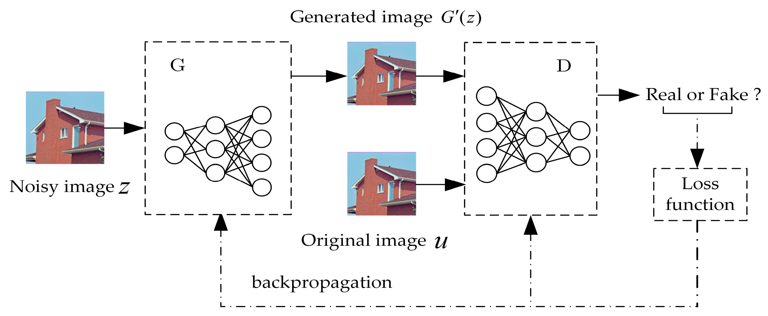
2.1. Generative Adversarial Network

The GAN is a deep learning model capable of producing high-quality outputs through the adversarial training of its Generator and Discriminator models within a framework. This network, introduced by Ian Goodfellow et al. [30] in their 2014 paper “Generative Adversarial Networks”, represents an unsupervised learning approach widely employed in tasks such as image denoising. Its structure is shown in Figure 1.
The noisy image z is input into the generator G , resulting in the acquisition of the generated image G ( z ) . The generated image G ( z ) is then fed into the discriminator D together with the original image u to output the probability that the generated image bearing resemblance to the original image. Finally, the loss function is adjusted in reverse and iteratively trained for both the generator network G and the discriminator network D . This iterative process aims to make the generated image G ( z ) from the generator network G closely resemble the original image. Simultaneously, it strives to make the discriminator D unable to accurately recognize the generated image from the original image. In other words, it seeks to achieve the optimal denoising effect through the generation network G .

2.2. Residual Learning

In light of the progress in deep learning techniques, more researchers are opting to increase the depth of neural networks to enhance model performance and extract more intricate image features for image denoising. However, studies have revealed that excessively deep networks often lead to information loss during feature extraction, negatively impacting image feature reconstruction. Consequently, He et al. [31] introduced the residual structure, where a skip connection forms a path between the input and output of each block, effectively addressing this issue. The residual block is illustrated in Figure 2.
Given an input F i and an output F i + 1 , where the convolution operation is denoted as H , the input-output relationship can be represented as follows:
F i + 1 = F i + H ( F i )
Within the context of the residual structure, the input F i undergoes a convolution operation, and the resulting outcome H ( F i ) is then added to the original input F i to yield the output F i + 1 of the residual module. In contrast to the output F i + 1 = H ( F i ) of the traditional CNN, the residual network primarily involves the calculation of a minor adjustment to the input F i . Subsequently, this adjustment is applied to transform the output H ( F i ) , resulting in a composition of both the original input F i and the magnitude of the calculated adjustment. By transferring information to deeper layers of the neural network through skip connections, it ensures that even in deeper networks, image features are retained. This effectively addresses the issues of gradient disappearance and gradient explosion, thereby stabilizing the network’s performance.

3. Design of Network Architecture and Denoising Model

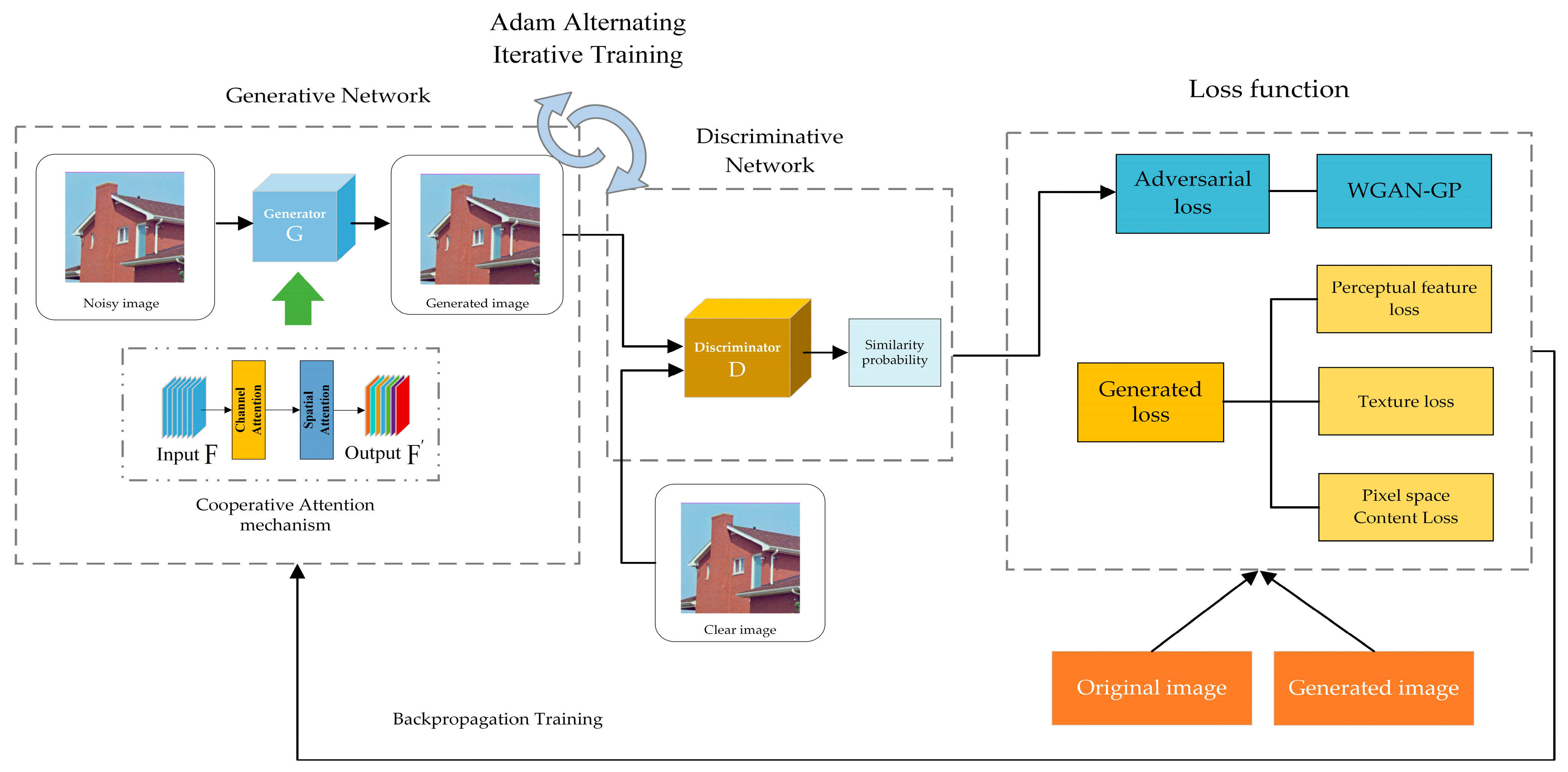
3.1. RCA-GAN Network Architecture

This paper introduces an image denoising approach based on GAN, referred to as RCA-GAN, which combines a Cooperative Attention mechanism with residual learning. The algorithm framework outlined in this study is visually depicted in Figure 3. Initially, the noisy image is fed into the generator G , which incorporates the Cooperative Attention mechanism, resulting in the generation of a reconstructed image. Subsequently, both the generated image and the original image are jointly provided as input to the discriminator D , which evaluates the likelihood of the input image being similar to the original image. Finally, network parameter optimization is guided using a composite loss function that combines adversarial loss and generation loss with appropriate weighting. The iterative training of both the generator G and discriminator D incorporates the utilization of the Adam momentum optimizer. The purpose of this process is to refine the generated images, bringing them closer to the original images, ultimately resulting in the training of a generator model with enhanced denoising performance.

3.1.1. Generator Network Architecture

The generator network, serving as the core component of the denoising model, is primarily tasked with generating a low-noise image that faithfully preserves edge details, given a high-noise input image. This network operates through the cooperative action of the Cooperative Attention module and residual modules, facilitating the extraction of high-level features. The residual network retains more image details during convolution and pooling operations, enabling each channel to capture richer features for subsequent feature fusion. At the same time, the Cooperative Attention module assigns greater weights to crucial image textures and edge features, thereby enhancing high-frequency texture information and optimizing feature utilization. Consequently, this process brings the generated images closer to the original images. The improved generator network model is illustrated in Figure 4. In this context, k denotes the size of the convolution kernel, while n corresponds to the quantity of output channels allocated for the convolutional layer. s stands for the step size employed in the process, and C o n v refers to the convolutional layer itself. Additionally, B l o c k signifies the presence of the residual block, and B N is associated with the batch normalization process. The network comprises four modules: the feature extraction section, the feature domain denoising section, the high-level feature extraction section, and the feature dimensionality reduction fusion section.
The feature extraction section comprises multi-scale convolutional layers with kernel dimensions of 1 × 1, 3 × 3, 5 × 5, and 7 × 7, primarily employed to extract a sufficient number of features for subsequent network processing. The denoising component in the feature domain comprises a stack of eight convolutional layers, each followed by Batch Normalization (BN) layers and Rectified Linear Unit (ReLU) activation functions to enhance learning and accelerate network training. In the high-level feature extraction layer, an initial convolutional network is employed to fuse the denoising features, facilitating the subsequent extraction and processing of abstract high-level features. These convolutional layers contribute to capturing intricate patterns and minute details within the image. Following this initial fusion, a stack of residual blocks is utilized to further extract and multidimensionally fuse the denoising features. Leveraging skip connections, this combination enhances the network’s ability to model high-frequency image details by merging the abstraction capacity of high-dimensional features with the information preservation capability of low-dimensional features. RCA-GAN incorporates a Cooperative Attention mechanism before the residual structure, aiming to thoroughly explore key feature information such as edges and textures. It assigns higher weights to these critical features while suppressing relatively redundant or less important characteristics, thereby reducing the weight allocated to such information. The Cooperative Attention mechanism enhances the recovery capacity for image detail and edge information by allocating different weights selectively. Simultaneously, the inclusion of the attention module helps mitigate some noise in the skip connections, further contributing to denoising. Additionally, the residual network addresses optimization challenges linked to increased network depth, averting network degradation through skip connections, and mitigating the risk of gradient explosion. The feature dimensionality reduction fusion part employs a five-layer stacked convolutional network to select and fuse image features from different levels, ultimately reducing the image features to a single-channel image as the output. Finally, global cross-layer connections are employed to compensate for detail loss in the output image by utilizing information from the input image. The generated denoised image is subsequently reconstructed by mapping the output image to the pixel value range that aligns with it using the tanh activation function.

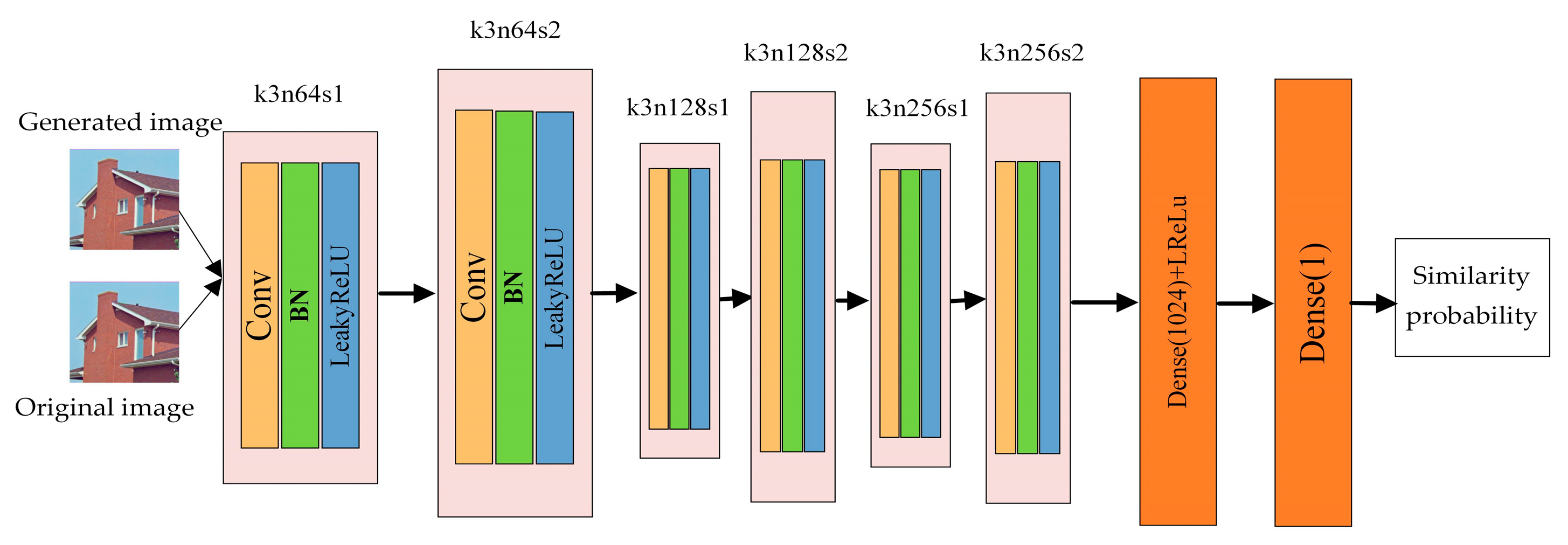
3.1.2. Discriminator Network Architecture

The discriminator network is constructed using a fully convolutional neural network, which serves the purpose of distinguishing whether the input image is an original real image or a generated image. By employing two different convolution kernel sizes for feature extraction and fusion, maximum pooling is chosen for image down-sampling, thus preserving more texture details. The architecture of the discriminator network is depicted in Figure 5.
Where k, n, and s represent the size of the convolutional kernel, number of channels, and step size, respectively. The discriminant network consists of six convolutional layers, followed by two fully connected layers. The input image is extracted and fused through six stacked convolutional layers. Each convolutional layer is processed with batch normalization and utilizes the Leaky Rectified Linear Unit (LReLU) activation function. Additionally, maximum pooling is employed for image down-sampling operations to retain more texture details. The quantity of kernels in the convolutional layer is increased, and the features are doubled each time. Two different step sizes for convolutions are employed to reduce the sharpness of the image. The final step involves processing the extracted 256 feature maps through two fully connected layers, with 1024 outputs in the first layer and a single output in the second layer. These fully connected layers handle the extracted features to determine the probability of the input image being similar to a real image. The 1024 outputs refer to the output dimension of the first fully connected layer, representing the information captured by the discriminator network at a high-level feature hierarchy. This layer of a fully connected network is employed for further processing the feature maps extracted from the convolutional layers, enhancing the network’s capability to distinguish between real and generated images. The purpose of using feature maps is to provide the discriminator with a rich feature representation, effectively distinguishing between original real images and generated images. Each feature map captures different aspects of the input image, enabling the network to consider a wide range of features in the decision-making process. The choice of the number of feature maps is typically determined based on various factors and experimental results. In this experiment, the use of 256 feature maps is considered a sufficient quantity to strike a balance between model complexity and performance. The cross-entropy layer is omitted at the end of the discriminator, and image patches are utilized for image training. The omission of the cross-entropy layer is a carefully considered decision stemming from the distinct nature of the discriminator’s role in GAN compared to traditional classification tasks. In traditional classification problems, cross-entropy loss is typically used to measure the disparity between predicted results and actual class labels. However, in the context of GANs, the primary task of the discriminator is not image classification but rather the identification of differences between generated images and real images. The crux of GAN training lies in the adversarial loss, which establishes a competitive adversarial relationship between the generator and discriminator, differing from conventional classification losses. The loss functions employed in this model already encompass adversarial losses. Therefore, the omission of the cross-entropy layer is a prudent choice based on the specific task and structure of GAN.

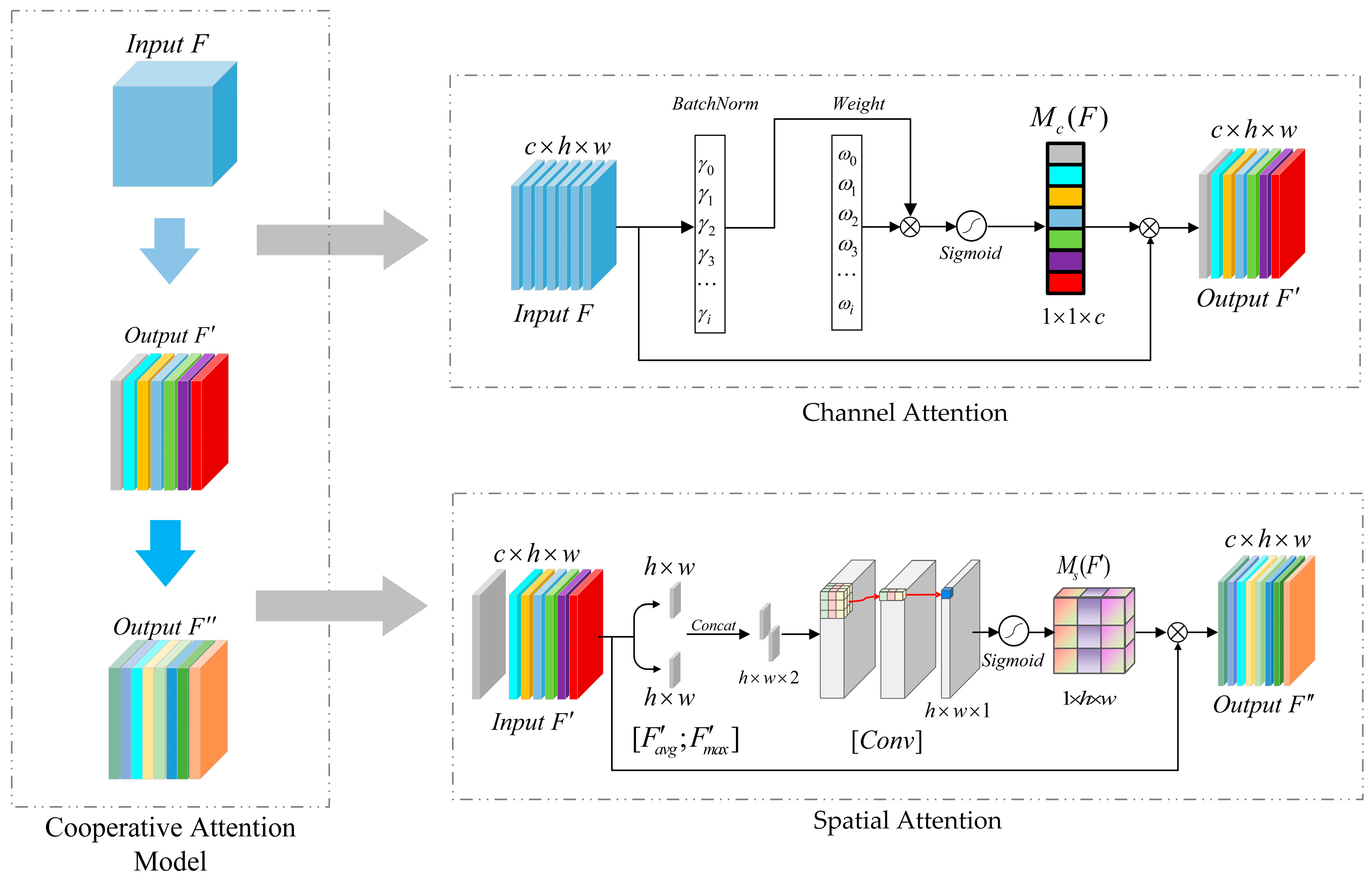
3.2. Cooperative Attention Mechanism

In the process of image denoising, image features can be categorized into key features (such as image edge features or texture features) and secondary features (such as redundant features). Traditional CNN [32,33,34,35] networks cannot effectively denoise images by extracting features since they fail to identify critical feature information. Attention mechanisms [36] address this issue by assigning higher weights to key features. In the literature [37], attention mechanisms and multi-scale feature fusion are employed to recover more image details. In [38], an adaptive attention module is utilized to extract image features while preserving more texture details in the images.
The channel attention mechanism dynamically modulates the weights of individual channels to enhance the representation capacity of channel features; however, it often overlooks crucial positional information. On the other hand, the spatial attention mechanism can adaptively choose the regions of interest, thereby preserving positional information. Therefore, this paper adopts a Cooperative Attention mechanism that combines channel attention and spatial attention. By leveraging the spatial attention structure to complement the shortcomings of the channel attention structure, it performs weighted processing on the input features in both spatial and channel dimensions, thereby enhancing the perceptual capabilities of features in spatial and channel dimensions, allowing for the exploration of more valuable information.
The Convolutional Block Attention Module (CBAM) [39] is a convolutional neural network model employed in the domain of computer vision, and it has demonstrated commendable results in visual tasks such as image classification and object detection. However, due to the multiple instances of pooling and dimension-reduction operations used within CBAM, it leads to the loss of vital information related to the spatial orientation and spatial attributes within images, which significantly affects the preservation of fine-grained texture details in the generated images. Therefore, this paper, drawing inspiration from CBAM, introduces a straightforward yet highly effective Cooperative Attention mechanism. This mechanism is integrated into the context of image denoising tasks within generative adversarial networks with the primary goal of extracting concealed noise information within complex backgrounds and enhancing the learning of image edges and texture features. The Cooperative Attention mechanism proves to be particularly proficient at addressing intricate noise distributions, enabling the modeling and processing of complex noise patterns within images, ultimately leading to a more accurate reconstruction of the original image information. In the case of handling noise with non-linear spatial correlations, the Cooperative Attention mechanism can perform varying degrees of weighted processing based on the intensity and location of the noise, thereby enhancing the utilization of feature information. Therefore, the introduction of the Cooperative Attention mechanism in RCA-GAN enables high-dimensional feature extraction for addressing both hidden noise and complex background noise. This not only improves denoising performance but also effectively preserves the fine texture details in the image. In the CBAM module, the conventional channel attention mechanism often employs dimensionality reduction operations on image features, which can lead to the loss of texture details in the channel dimension and a decrease in the efficiency of capturing interdependencies between channels. Therefore, this paper introduces improvements to the channel attention component. In contrast to the traditional channel attention module in the CBAM module, our approach adopts a strategy that does not reduce feature dimensions within the channel attention structure. Simultaneously, it retains the spatial attention component. By effectively combining the strengths of channel attention and spatial attention, our method focuses on critical image features while suppressing responses in unnecessary regions. The structural diagram of the Cooperative Attention mechanism model is presented in Figure 6.
When dealing with the input feature map F R c × h × w , the initial step involves calculating a one-dimensional attention weight matrix M c ( F ) R 1 × 1 × c using the enhanced channel attention module. Subsequently, a two-dimensional spatial attention weight matrix M s ( F ) R 1 × h × w is computed through the spatial attention module. These matrices are then utilized to derive the final enhanced feature maps, relying on attention weights. The entire process can be succinctly summarized using Equations (2) and (3). The channel attention module explicitly models the interdependencies among channels, thereby enhancing the feature representation of channels. To avoid the loss of high-dimensional information and mitigate the computational complexity resulting from an excessive number of parameters, this paper removes the fully connected layer and convolutional layer associated with traditional attention within the channel attention module. The process solely relies on batch normalization to compute the mean and variance across the channel. Additionally, it employs the learnable parameter γ to gauge the variance of each channel, signifying their individual importance. Subsequently, once the channel attention module conducts batch normalization on the input feature map F R c × h × w , it yields the channel attention weight matrix M c ( F ) . This matrix is then utilized to perform element-wise multiplication with the input feature map F , resulting in the weighted feature map F . The computation procedure for channel attention is detailed in Equations (4) and (5).
F = M c ( F ) F
F = M s ( F ) F
B N ( B i n ) = γ B i n μ I σ I 2 + τ + β
M c ( F ) = S i g m o i d ( γ i j = 0 γ j ( B N ( F ) ) )
where represents the pointwise matrix multiplication operation, μ I and σ I are the mean and standard deviation of the current batch I , respectively, while γ and β are designated as trainable scaling factors and displacements. Additionally, the hyperparameter τ serves as the minimal value introduced to prevent the denominator from reaching zero.
Based on the channel attention module, this paper employs a spatial attention mechanism to learn inter-feature correlations, thus capturing dependencies among feature regions. Within the spatial attention module, two critical operations take place: channel-based global maximum pooling F m a x and global average pooling F a v g . These operations are applied to the feature map F R c × h × w , which is the output from the Channel Attention module, along the channel dimension. Consequently, two two-dimensional maps, denoted as F m a x R 1 × h × w and F a v g R 1 × h × w , are generated through these pooling operations. By combining these two maps through concatenation, the module achieves the aggregation of feature map channel information and the selection of spatial information. Subsequently, by employing a convolution operation, the dimensionality is reduced to a single channel to derive the spatial attention weight matrix. Following this step, the Spatial Attention Map, which is the spatial weight matrix M s ( F ) , is generated through the Sigmoid activation layer. In the final step, the weight matrix output from the spatial attention module is multiplied with the input features to facilitate adaptive feature refinement. This step encourages the model to focus more on crucial information within the input features while attenuating less important details, consequently enhancing the model’s performance. The aforementioned process can be represented as Equation (6).
M s ( F ) = S i g m o i d ( f 7 × 7 ( [ F a v g ; F m a x ] ) )
In this context, f 7 × 7 signifies the convolution operation employing a 7 × 7 convolution kernel.

3.3. Multimodal Loss Function

In order to consider more texture detail information, this paper utilizes the weighted sum of perceptual feature loss, pixel space content loss, texture loss, and the adversarial loss is employed iteratively to fine-tune the network for achieving an improved denoising effect. The total loss function in this paper is defined as follows:
L l o s s = λ 1 L percep   + λ 2 L c o n + λ 3 L t e x + λ 4 L W G A N - G P
In the equation, λ 1 , λ 2 , λ 3 and λ 4 represent the weight of each loss, respectively. L percep   stands for perceptual feature loss; L c o n stands for pixel space content loss; L t e x stands for texture loss; L W G A N G P stands for adversarial loss. L percep   , L c o n , and L t e x are calculated as follows:
L percep   = ϕ I R I ϕ G I D I 2 2
L c o n = G ( I D I ) I R I 1 2 + ε 2
L tex   = Gram ϕ G I D I Gram ϕ I R I 2 2
In the equation, . 1 represents L1 norm, . 2 represents the L2 norm, ϕ denotes the feature extractor, I D I represents the noisy image, I R I represents the original image, and G . represents the generator network. Gram represents the Gram matrix, which is used to describe the texture information of an image. The Gram matrix allows for the reconstruction of fine texture details in an image.
RCA-GAN incorporates Wasserstein Generative Adversarial Network with Gradient Penalty (WGAN-GP), an enhanced iteration of WGAN’s discriminative loss, as the adversarial loss function for network training. The utilization of Wasserstein distance effectively addresses issues encountered in the original GAN network. Simultaneously, WGAN-GP proves to be effective in quantifying the distance between two data distributions, and its optimization objective function is depicted in Equation (11).
L W G A N - G P ( D ) = E u P d a t a [ D ( u ) ] + E u P g [ D ( u ) ] + λ E u ^ P u ^ [ u ^ D ( u ^ ) 2 1 2 ]
In the equation, E(⋅) represents the expectation operator, P d a t a stands for the original data distribution, P g represents the generated data distribution, D . represents the discriminator network, P u ^ is a random sample drawn from the space between P d a t a and P g , and u ^ D ( u ^ ) 2 signifies the gradient of the discriminator network. WGAN-GP stabilizes the gradient of the discriminant network by adding an additional loss on the basis of WGAN.

4. Experimental Comparisons and Analysis

4.1. Data Set

In this study, the Berkeley Segmentation Dataset 400 (BSD400) and Berkeley Segmentation Dataset and Benchmark500 (BSDS500) datasets [40], provided by the University of California, Berkeley, were used as training datasets for grayscale and color images, respectively. Due to the limited number of images in the training datasets, which were insufficient for network optimization, Gaussian white noise with mean zero and standard deviations of σ = 15, σ = 25, and σ = 50 was initially added to 500 color images from BSDS500, resulting in a dataset of 1500 noisy images. Subsequently, 3000 blurred, noisy image pairs were generated by applying image flipping, creating clear-noisy image pairs for training the color image denoising model. Additionally, the 400 grayscale images from BSD400 underwent the same data augmentation procedures, resulting in a final set of 2400 clear-noisy image pairs for training the grayscale image denoising model. The classic Color Set8 (CSet8) and Berkeley Segmentation Dataset 68 (BSD68) datasets [41] were employed to evaluate denoising performance on grayscale and color images, respectively. The training and testing datasets used in this study were mutually independent, with no dependencies between them. The effectiveness of the denoising algorithm for noisy images was validated through denoising tests conducted on the testing dataset.
In our experiments, we employed Gaussian noise to simulate the unknown real-world noise more accurately. In real environments, noise is often not caused by a single source but is a complex mixture of noise from various sources. If we consider real noise as the aggregation of random variables with different probability distributions, and each random variable is independent, then, according to the Central Limit Theorem, as the number of noise sources increases, their normalization tends to follow a Gaussian distribution. Based on this assumption, using synthesized Gaussian noise offers a straightforward and realistic approximation for addressing complex situations in which the noise distribution is unknown.
Data augmentation is a commonly employed deep learning training strategy used to generate more data from a limited set of original data by creating transformed versions of training samples. Its purpose is to enhance a model’s generalization capability. This technique encompasses various methods, including flipping, scaling, and rotation. In particular, flipping aids the model in learning spatial invariance within images from different perspectives, thus improving its generalization ability. Flipping allows the model to better comprehend images from various orientations, thereby enhancing its adaptability to variations.

4.2. Experimental Environment

The hardware and software environment configurations used in all experiments in this paper are shown in Table 1 and Table 2.

4.3. Evaluation Metrics

4.3.1. PSNR

Peak Signal-to-Noise Ratio (PSNR) is the most commonly used image quality assessment standard. It is employed to quantify the denoising performance of a model when ground truth noise-free images are available. PSNR is based on the magnitude of the Mean Square Error (MSE), which measures the pixel-wise differences between the denoised image and the ground truth image. The calculation equations for MSE and PSNR are provided in Equations (12) and (13), respectively.
MSE = 1 M × N i = 1 M j = 1 N X i j Y i j 2
PSNR = 10 log 10 n 2 MSE ( X , Y )
where, X i j and Y i j represent the pixel values in noise-free images of size M × N and noisy images, respectively. i and j denote the coordinates of the pixels within the image positions. n represents the maximum grayscale level of the image.

4.3.2. SSIM

Structural Similarity Index (SSIM) is a metric used to assess image similarity by considering multiple features, including contrast, brightness, and structure, making it a more objective image denoising evaluation indicator. The calculation process of SSIM is presented in Equations (14) and (15).
l ( X , Y ) = 2 μ X μ Y + C 1 μ X 2 + μ Y 2 + C 1 c ( X , Y ) = 2 σ X σ Y + C 2 σ X 2 + σ Y 2 + C 2 s ( X , Y ) = σ X Y + C 3 σ X σ Y + C 3
SSIM ( X , Y ) = l ( X , Y ) c ( X , Y ) s ( X , Y )
where X and Y represent the two images involved in structural similarity comparison, while l ( X , Y ) , c ( X , Y ) , and s ( X , Y ) , respectively, denote the similarity in luminance, contrast, and structure of the images. μ X and μ Y represent the pixel means of two images, while σ X and σ Y represent the pixel standard deviations of the two images. σ X Y stands for the covariance between the two images. C 1 , C 2 , and C 3 are all constants, ensuring the validity of the structure by avoiding a zero denominator. Where C 1 = ( K 1 × L ) , C 2 = ( K 2 × L ) , and C 3 = ( C 2 / 2 ) , under normal circumstances, take on the values K 1 = 0.01, K 2 = 0.03, and L = 255.

4.4. Experimental Results

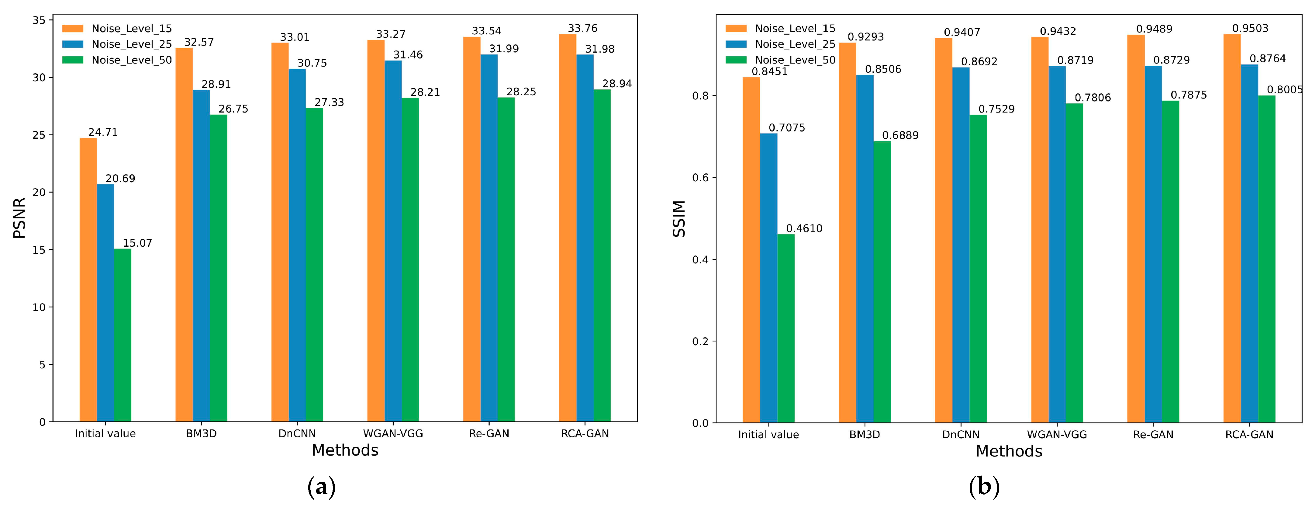
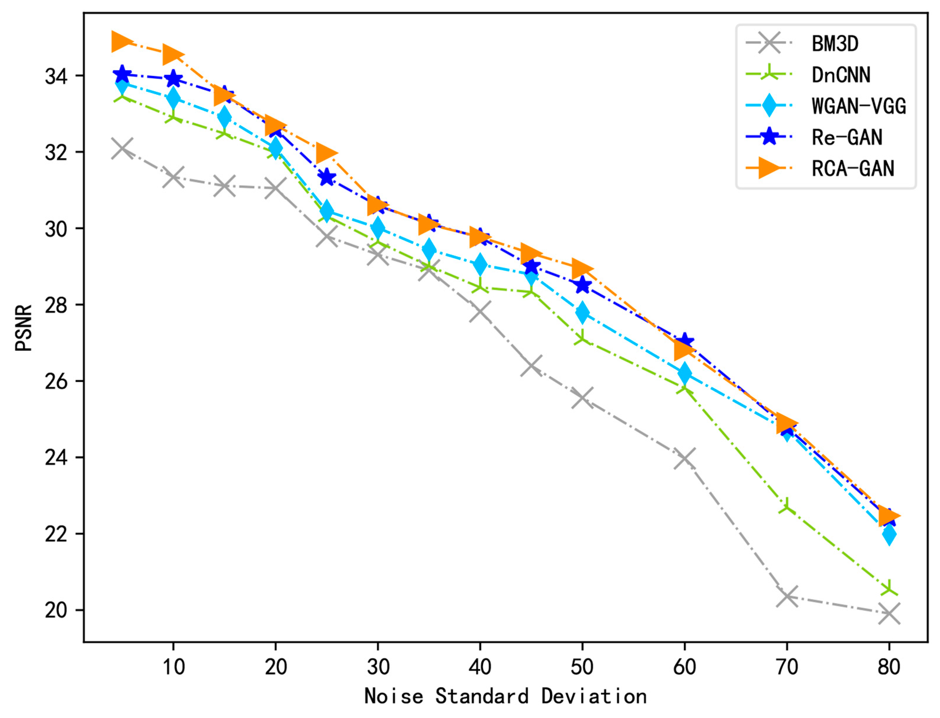
4.4.1. Quantitative Analysis

In this paper, some representative Block-Matching and 3D Filtering (BM3D) [21], DnCNN [23], Wasserstein Generative Adversarial Network with VGG Loss (WGAN-VGG) [28], and Residual-Generative Adversarial Network (Re-GAN) [42] are used as comparison algorithms, and Gaussian white noise with noise intensity σ of 15, 25 and 50 is added to the BSD68 dataset, respectively. The PSNR and SSIM of different image denoising methods are illustrated in Table 3. For a more intuitive representation, Figure 7 describes the PSNR values of different algorithms in the form of a bar chart under varying levels of noise intensity. The values of PSNR and SSIM represent the average results of all images in the entire dataset. The experimental data obtained in the table shows that the denoising effect of the algorithm proposed in this paper surpasses that of other comparable algorithms to a significant extent under different noise intensities, and both PSNR and SSIM have been improved to varying degrees.
When the noise intensity is set to σ = 15, the application of the algorithm proposed in this paper results in an impressive average increase of 9.05 dB in PSNR value after denoising. In direct comparison with the BM3D algorithm, both the PSNR and SSIM values show notable improvements, increasing by 3.7% and 2.3%, respectively. Similarly, in comparison to the fundamental DnCNN algorithm, the PSNR value and SSIM value demonstrate improvements of 2.3% and 1.0%, respectively. In contrast with WGAN-VGG, the PSNR value and SSIM value experience enhancements of 1.5% and 0.8%, respectively. Lastly, in comparison to Re-GAN, the PSNR value and SSIM value show increases of 0.7% and 0.1%, respectively. Notably, experimental data reveals that even when noise intensity remains relatively low, RCA-GAN consistently exhibits strong denoising capabilities, particularly in scenarios where differences between deep learning methods are not substantial.
When the noise intensity is set to σ = 25, the denoising capabilities of RCA-GAN far exceed those of the initial three denoising algorithms. In direct comparison to the denoising outcomes achieved by BM3D, DnCNN, and WGAN-VGG, the PSNR value exhibits substantial improvements, increasing by 10.6%, 4.0%, and 1.7%, respectively. Interestingly, the average PSNR value after applying the RCA-GAN denoising method is marginally lower than that of the Re-GAN algorithm. This suggests that the disparities in pixel values between the two resulting images are not particularly conspicuous. However, when evaluating structural similarity, it becomes evident that RCA-GAN surpasses Re-GAN by a margin of 0.4%. This signifies superior visual performance in images denoised by the algorithm presented in this paper.
At a noise intensity level of σ = 50, RCA-GAN demonstrates notably enhanced content integrity and improved structural similarity. In direct comparison to the BM3D algorithm, both the PSNR and SSIM values exhibit substantial increases, showing improvements of 8.2% and 16.2%, respectively. Similarly, when compared to the fundamental DnCNN method, both the PSNR value and SSIM value experience significant enhancements, demonstrating improvements of 5.9% and 6.3%, respectively. In contrast, when pitted against WGAN-VGG, the PSNR value and SSIM value demonstrate appreciable improvements of 2.6% and 2.5%, respectively. Additionally, compared to the Re-GAN algorithm, both the PSNR value and SSIM value register increases of 2.4% and 1.7%, respectively. What stands out is that, unlike scenarios with low noise, it becomes evident that the approach proposed in this paper exponentially augments the denoising effect in cases characterized by high noise intensity.
Apart from common metrics like PSNR and SSIM, time complexity is also an important criterion for evaluating image denoising algorithms. To clearly demonstrate the complexity of different algorithms, multiple experiments were conducted using images with a noise standard deviation of 15 and a resolution of 256 pixels × 256 pixels. The average execution times for different algorithms were obtained, and Table 4 presents the average runtime of different denoising algorithms. From the data in Table 4, it is evident that in a CPU runtime environment, RCA-GAN reduces the average denoising time by 8.06 s compared to BM3D, by 2.02 s compared to DnCNN, by 1.15 s compared to WGAN-VGG, and by 0.58 s compared to Re-GAN. In a GPU runtime environment, RCA-GAN exhibits a 35.3% improvement in average denoising efficiency compared to DnCNN, a 26.7% improvement compared to WGAN-VGG, and a 21.4% improvement compared to Re-GAN. In comparison to other deep learning denoising algorithms, our algorithm enhances effective feature utilization by incorporating an attention mechanism while reducing the number of feature extraction layers and residual blocks. This reduces computational complexity compared to traditional convolutional layers and enhances processing speed. Therefore, our algorithm demonstrates superior performance in terms of runtime.
In comparison to other conventional algorithms, although our algorithm excels in terms of the average denoising time per single image, it is important to note that our algorithm’s training time is relatively prolonged. This situation primarily arises from the utilization of the Deep GAN architecture, which demands a substantial number of training iterations and computational resources. Particularly, when handling high-resolution images or extensive datasets, the training time may experience significant extensions. While the extended training time stands as a limitation of our algorithm, it is imperative to recognize that this challenge is prevalent within the current domain of deep learning methodologies. Future endeavors may be directed toward further optimizing the training process, enhancing computational efficiency, and exploring swifter model architectures to augment the feasibility of our algorithm. We acknowledge this aspect and encourage prospective research to persistently refine and advance the technologies within this field to overcome the temporal constraints.
To ensure the experiment’s rigor, this study assesses the denoising effectiveness of RCA-GAN within a specific range of noise intensities. Initially, noise is incrementally added to the same test set image, commencing from a noise intensity of σ = 5, and progressing to a maximum noise intensity of σ = 80 (beyond which image repair becomes nearly impossible). This process yields a total of 13 noisy images. Subsequently, each of the five denoising models introduced in this paper is applied to denoise the aforementioned noisy images individually. Finally, the PSNR and SSIM values of the denoised images are computed to objectively evaluate the denoising capabilities of the RCA-GAN model. Figure 8 and Figure 9 depict the change curves in PSNR and SSIM values for each algorithm model within the specified range of noise intensities following image denoising.
The experimental results reveal that RCA-GAN exhibits enhanced PSNR and SSIM metrics in comparison to other benchmark algorithms. Consequently, with the incorporation of the mixed attention mechanism, RCA-GAN demonstrates superior capabilities in preserving image details while effectively eliminating noise.

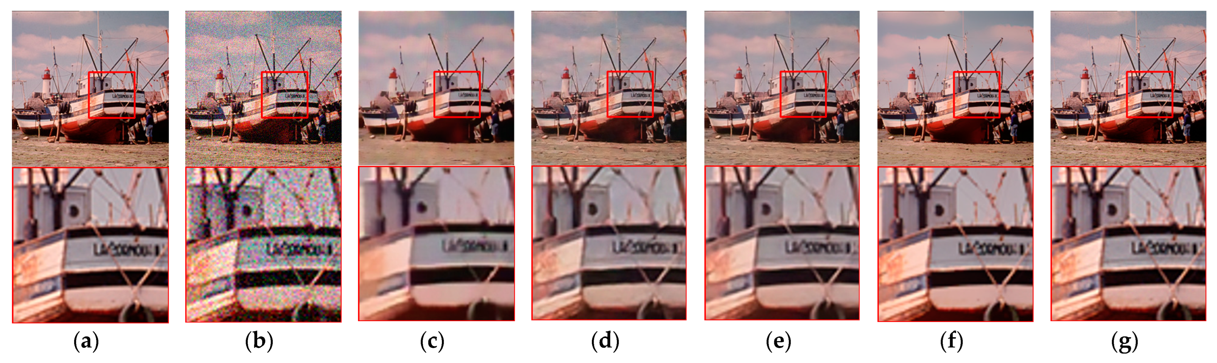
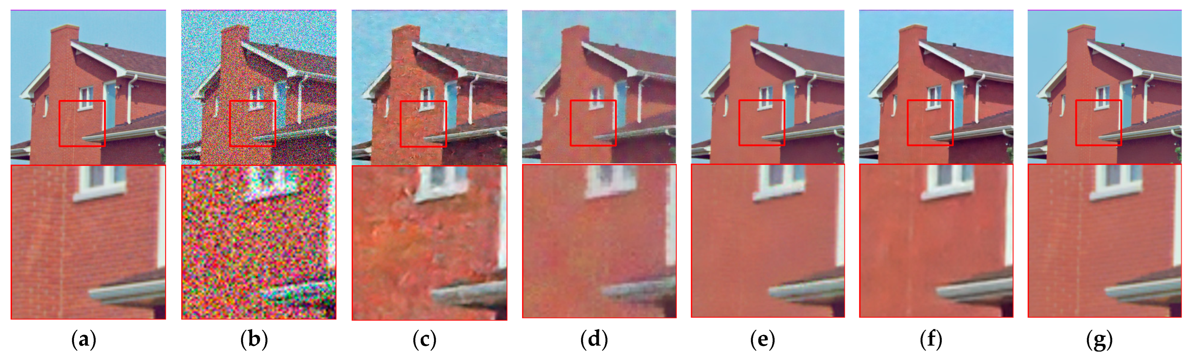
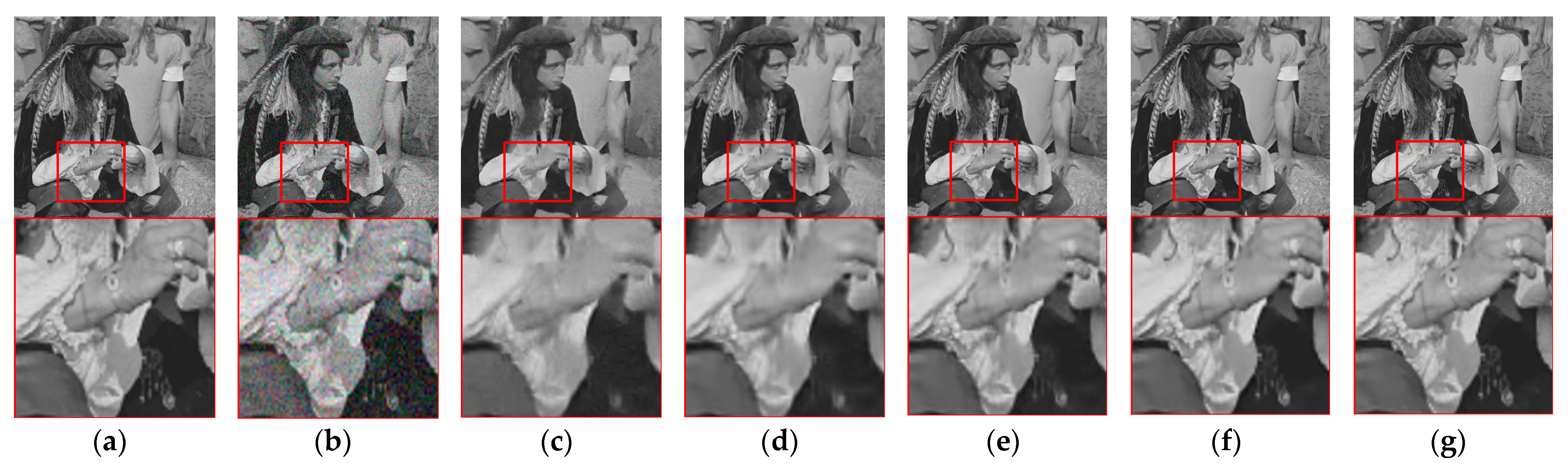
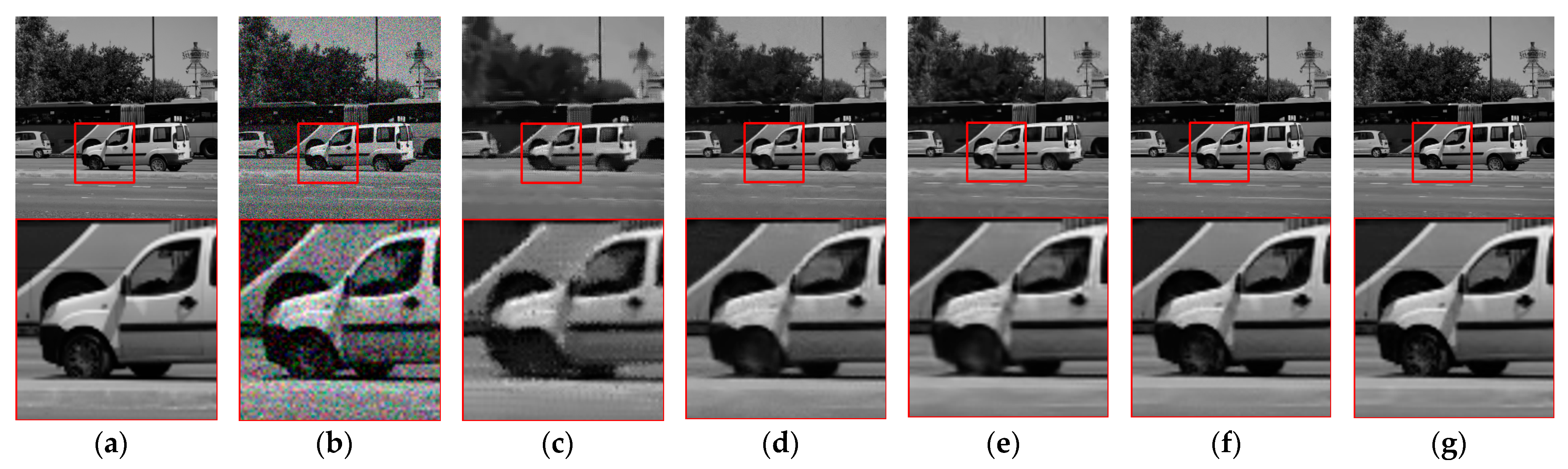
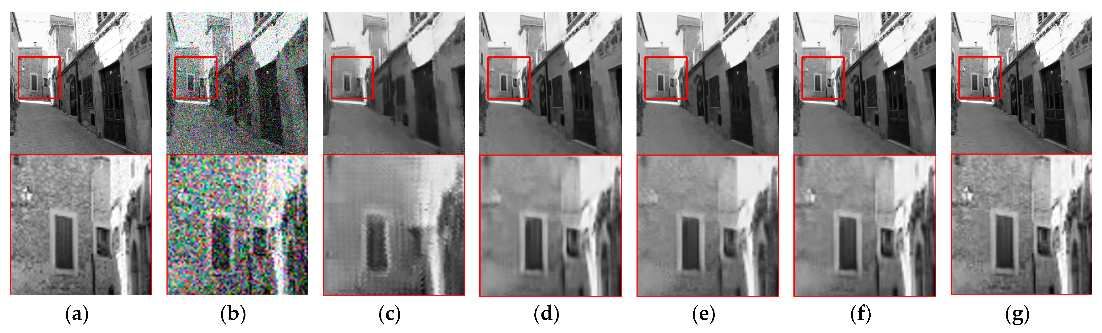
4.4.2. Qualitative Analysis

When evaluating denoising effects, subjective impressions are as crucial as objective experimental data. To comprehensively assess the disparities between our proposed approach and the comparison algorithms, we selected two images—Barbara and Boats—from the CSet8 test set. These images were subjected to different levels of Gaussian white noise ( σ = 25, 50) to evaluate denoising outcomes, as depicted in Figure 10 and Figure 11.
Figure 10 illustrates the denoising visual outcomes of the Boats image, alongside results obtained using other denoising algorithms, at a noise intensity of σ = 25. Upon close examination, it becomes evident that the traditional denoising algorithm BM3D effectively eliminates noise from the entire image. However, the processed image exhibits noticeable blurriness, resulting in a loss of vital image detail information. In the case of DnCNN and WGAN-VGG, their denoising processes introduce a blurred smoothing effect along the edges of the image. Meanwhile, Re-GAN succeeds in preserving a greater amount of detailed information, and its visual results closely resemble those produced by the algorithm presented in this paper. Nevertheless, upon closer scrutiny of enlarged detail areas, the algorithm proposed in this paper demonstrates superior capabilities in retaining image texture, edge definition, and other critical details, ultimately leading to enhanced visual effects.
Figure 11 illustrates the denoising visual results of the House image with a noise intensity of σ = 50 in comparison to other benchmark algorithms. From Figure 10, it is evident that as noise intensity increases, the traditional denoising algorithm BM3D struggles to effectively address the denoising task. DnCNN, while affected by noise, mistakenly preserves noise as useful information. WGAN-VGG and Re-GAN, though proficient at removing noise, overly smooth the image’s structure, resulting in a loss of fine texture details in the denoised images. In contrast, employing our proposed algorithm, RCA-GAN, not only retains a relatively higher level of fine detail information but also presents a clearer overall visual perception that closely resembles the original image. This demonstrates that our algorithm excels in effective noise removal while preserving more image texture details, showcasing its robust denoising performance.
The RCA-GAN model additionally chooses three monochrome images from the BSD68 dataset—Man, Traffic, and Alley—for testing and visualization purposes. The denoising effect diagrams for these images are presented in Figure 12, Figure 13 and Figure 14.
As demonstrated in the sleeve portion of the Man image within Figure 12g, it becomes evident that RCA-GAN achieves significantly higher image clarity and texture quality after denoising at low noise intensity, surpassing the performance of DnCNN and WGAN-VGG. Likewise, in the leafy region at the top-left corner of the Traffic image featured in Figure 13g, encompassing the outline of the white car and the shadow effects of the car door handle, RCA-GAN exhibits impressive pixel retention capabilities under medium noise intensity. Further observations, illustrated by the enlarged wall section in the Alley image showcased in Figure 14g, reveal that the RCA-GAN model excels in restoring texture details and preserving edge structures. Collectively, the experimental results establish that the RCA-GAN model excels in reconstructing intricate image features and texture characteristics while effectively reducing noise, thereby enhancing the quality and content accuracy of the generated image.

4.4.3. Loss Function Ablation Experiments

In the context of image denoising, the selection of a loss function significantly impacts the retention of textural intricacies within the denoised image. To assess the efficacy of the loss function in this study, the RCA-WGAN network is fine-tuned and trained using five distinct loss functions, including MSE and LWGAN-GP. An ablation experiment of the loss function is then conducted using the same test set images and identical noise intensity levels. The outcomes of these experiments are shown in Table 5.
Under the Gaussian white noise with noise intensity σ = 15, the proposed Multimodal Loss Function improves the PSNR by 7.0%, 5.3% and 4.4%, and the SSIM by 2.6%, 1.2% and 0.3%, respectively, compared to MSE, L W G A N - G P and L percep   + L W G A N - G P . After adding L t e x texture loss to the above loss function, the results show a slight decrease in PSNR values, but the denoised images are closer to the original images with regard to luminance, contrast, and structural characteristics, showing good denoising effects.

4.4.4. Analysis of Different Weight Coefficients in the Loss Function

In this experiment, the optimal combination of weighting factors for the Multimodal Loss Function was determined through multiple iterations. These weighting factors included perceptual feature loss, pixel space content loss, texture loss, and adversarial loss. The ideal set of weighting values, which resulted in the best performance in terms of evaluation metrics, was found to be λ 1 = 1.0, λ 2 = 0.01, λ 3 = 0.001, and λ 4 = 1.0, respectively. This specific set of weight values enabled our model to achieve its peak performance across various performance indicators. A quantitative comparison of denoising results with different weight coefficients for the loss function is presented in Table 6.
The adjustment of the perceptual feature loss weight impacts the perceptual quality and structural characteristics of the image. A lower weight leads to insufficient optimization of the network for the perceptual features of the input image, thereby affecting the quality and structural characteristics of the reconstructed image. Conversely, increasing the weight of the perceptual feature loss encourages the model to focus more on pixel-level details. Nevertheless, this might introduce some high-frequency noise, resulting in a decreased PSNR value.
When the weight of pixel space content loss is increased, the PSNR values demonstrate a relatively stable trend, signifying the preservation of pixel-level similarity. Nonetheless, we observe alterations in SSIM values, indicating a minor compromise in the model’s capacity to maintain the image’s structural and semantic information. This outcome highlights the delicate balance in weight settings, in which an elevation in pixel space content loss weight aids in conserving pixel-level similarity while concurrently diminishing structural similarity in the image.
Texture loss is intended to capture the details and textures within an image, and an increase in its weight encourages the model to focus more on these specific features. However, this adjustment can introduce high-frequency noise, leading to a reduction in pixel-level similarity and causing fluctuations in pixel-level comparisons. Simultaneously, we also observed slight variations in SSIM values, suggesting that the model’s treatment of the image’s structural and semantic information was only minimally affected. Nevertheless, these variations did not demonstrate a significant trend.
When adjusting the weight of the adversarial loss, there was no significant change in image reconstruction quality with this weight modification. However, the decrease in SSIM is relatively more pronounced, indicating a certain reduction in the visual quality of the images. This is because adversarial loss plays a crucial role in the image generation process and is essential for maintaining the visual and perceptual quality of the images. Therefore, fine-tuning the weight of the adversarial loss has a critically important impact on improving the image generation quality of the model.

4.4.5. Analysis of Visual Tasks and Applications

In the context of Synthetic Aperture Radar (SAR) image processing, image denoising holds significant importance. SAR images are obtained by transmitting radar signals and receiving their echoes to gather information about the Earth’s surface, making them susceptible to interference from noise. If not subjected to denoising, the noise in SAR images can substantially impact the extraction and recognition of ground features, consequently affecting the effectiveness of image applications. This paper conducts model training using existing real noise datasets and applies the trained RCA-GAN model to denoise real noise in SAR images, thereby validating the effectiveness of RCA-GAN in handling real noise and enhancing its capability to address complex real-world scenarios. For this purpose, SAR images with lower noise intensity are used as the original images, while images with higher noise intensity are utilized as noise images from the same category. The denoising performance of the proposed algorithm is evaluated using objective metrics such as PSNR and SSIM. The results of the SAR image denoising are depicted in Figure 15.
In this context, the first SAR image affected by noise, after denoising with RCA-GAN, saw an increase in PSNR value from 15.83 dB to 27.46 dB, representing a 73.5% improvement. The SSIM value increased from 0.4210 to 0.7954, showing an 88.9% improvement. The second and third SAR images, after noise removal, exhibited increases of 51.9% and 58.6% in PSNR values, and 92.7% and 94.8% in SSIM values, respectively. Based on the analysis of experimental data, it is evident that the proposed RCA-GAN model is effective in handling complex real noise. Furthermore, in the denoising process of SAR images, the RCA-GAN model holds significant practical value.

5. Conclusions

In response to the issue of traditional denoising algorithms causing the loss of edge and fine-grained details in denoised images, this paper introduces an enhanced GAN-based image denoising algorithm called RCA-WGAN. RCA-WGAN integrates residual structures and a cooperative attention mechanism within the feature extraction component of the generator network. Additionally, it incorporates a global residual connection to capture more image features, effectively eliminating noise while preserving image details. To optimize noise reduction, a Multimodal Loss Function is formulated through weighted summation, encompassing perceptual feature loss, pixel space content loss, texture loss, and adversarial loss. Furthermore, the proposed denoising method leverages essential features in the RGB channels to mitigate texture loss resulting from the denoising procedure. Through comparisons with four mainstream denoising algorithms—BM3D, DnCNN, WGAN-VGG, and Re-GAN—the efficacy of the proposed algorithm in restoring image texture details is demonstrated. Experimental results highlight that this algorithm, with enhancements in the denoising network module and loss function module, exhibits remarkable denoising performance, as evidenced by objective evaluation metrics such as PSNR and SSIM values. In contrast to alternative algorithms, the proposed method excels at noise removal while preserving image texture details. Effectively addressing complex noise in real-world scenarios continues to pose a significant challenge in the denoising procedure. Future work will concentrate on further optimizations of RCA-WGAN to enhance its performance in complex noise reduction and real-time processing.

Author Contributions

Conceptualization, Y.W. and S.L.; methodology, M.H.; software, Y.W. and L.M.; validation, Y.W., S.L. and M.H.; formal analysis, Y.W.; investigation, S.L.; resources, M.H.; data curation, Y.W.; writing—original draft preparation, S.L. and L.M.; writing—review and editing, S.L.; visualization, Y.W. and L.M.; supervision, S.L.; project administration, Y.W.; funding acquisition, Y.W. All authors have read and agreed to the published version of the manuscript.

Funding

This research was funded by the Defense Industrial Technology Development Program (grant number JCKYS2020DC01).

Data Availability Statement

This paper used the BSD400 and BSDS500 dataset, and according to the research requirements, the original dataset was augmented with various levels of Gaussian white noise to expand the data and increase the amount of data. Data source: http://www.eecs.berkeley.edu/Research/Projects/CS/vision/grouping/BSR/BSR_bsds500.tgz (accessed on 7 October 2023).

Conflicts of Interest

The authors declare no conflict of interest.

References

  1. Ihara, S.; Saito, H.; Yoshinaga, M.; Avala, L.; Murayama, M. Deep learning-based noise filtering toward millisecond order imaging by using scanning transmission electron microscopy. Sci. Rep. 2022, 12, 13462. [Google Scholar] [CrossRef] [PubMed]
  2. Zhang, D.; Zhou, F. Self-Supervised Image Denoising for Real-World Images with Context-Aware Transformer. IEEE Access 2023, 11, 14340–14349. [Google Scholar] [CrossRef]
  3. Nawaz, W.; Siddiqi, M.H.; Almadhor, A. Adaptively Directed Image Restoration Using Resilient Backpropagation Neural Network. Int. J. Comput. Intell. Syst. 2023, 16, 74. [Google Scholar] [CrossRef]
  4. Vimala, B.B.; Srinivasan, S.; Mathivanan, S.K.; Muthukumaran, V.; Babu, J.C.; Herencsar, N.; Vilcekova, L. Image Noise Removal in Ultrasound Breast Images Based on Hybrid Deep Learning Technique. Sensors 2023, 23, 1167. [Google Scholar] [CrossRef] [PubMed]
  5. Zhou, L.; Zhou, D.; Yang, H.; Yang, S. Two-subnet network for real-world image denoising. Multimed. Tools Appl. 2023. [Google Scholar] [CrossRef]
  6. Feng, R.; Li, C.; Chen, H.; Li, S.; Gu, J.; Loy, C.C. Generating Aligned Pseudo-Supervision from Non-Aligned Data for Image Restoration in Under-Display Camera. In Proceedings of the IEEE/CVF Conference on Computer Vision and Pattern Recognition, Vancouver, BC, Canada, 17–24 June 2023; pp. 5013–5022. [Google Scholar]
  7. Han, L.; Zhao, Y.; Lv, H.; Zhang, Y.; Liu, H.; Bi, G. Remote Sensing Image Denoising Based on Deep and Shallow Feature Fusion and Attention Mechanism. Remote Sens. 2022, 14, 1243. [Google Scholar] [CrossRef]
  8. Wang, Z.; Ng, M.K.; Zhuang, L.; Gao, L.; Zhang, B. Nonlocal Self-Similarity-Based Hyperspectral Remote Sensing Image Denoising with 3-D Convolutional Neural Network. IEEE Trans. Geosci. Remote Sens. 2022, 60, 1–17. [Google Scholar] [CrossRef]
  9. Zhang, F.; Liu, J.; Liu, Y.; Zhang, X. Research progress of deep learning in low-dose CT image denoising. Radiat. Prot. Dosim. 2023, 199, 337–346. [Google Scholar] [CrossRef]
  10. Fan, L.; Zhang, F.; Fan, H.; Zhang, C. Brief review of image denoising techniques. Vis. Comput. Ind. Biomed. Art 2019, 2, 7. [Google Scholar] [CrossRef]
  11. Ismael, A.A.; Baykara, M. Digital Image Denoising Techniques Based on Multi-Resolution Wavelet Domain with Spatial Filters: A Review. Trait. Signal 2021, 38, 639–651. [Google Scholar] [CrossRef]
  12. Kostadin, D.; Alessandro, F.; Vladimir, K.; Karen, E. Image restoration by sparse 3D transform-domain collaborative filtering. Proc. SPIE 2008, 6812, 681207. [Google Scholar]
  13. Ma, Y.; Zhang, T.; Lv, X. An overview of digital image analog noise removal based on traditional filtering. Proc. SPIE 2023, 12707, 665–672. [Google Scholar]
  14. Kumar, A.; Sodhi, S.S. Comparative Analysis of Gaussian Filter, Median Filter and Denoise Autoenocoder. In Proceedings of the 2020 7th International Conference on Computing for Sustainable Global Development (INDIACom), New Delhi, India, 12–14 March 2020; pp. 45–51. [Google Scholar]
  15. Wu, J. Wavelet domain denoising method based on multistage median filtering. J. China Univ. Posts Telecommun. 2013, 20, 113–119. [Google Scholar] [CrossRef]
  16. Lu, C.-T.; Chen, M.-Y.; Shen, J.-H.; Wang, L.-L.; Yen, N.Y.; Liu, C.-H. X-ray bio-image denoising using directional-weighted-mean filtering and block matching approach. J. Ambient Intell. Humaniz. Comput. 2018, 1–18. [Google Scholar] [CrossRef]
  17. Erkan, U.; Thanh, D.N.H.; Hieu, L.M.; Enginoglu, S. An Iterative Mean Filter for Image Denoising. IEEE Access 2019, 7, 167847–167859. [Google Scholar] [CrossRef]
  18. Feng, X.; Zhang, W.; Su, X.; Xu, Z. Optical Remote Sensing Image Denoising and Super-Resolution Reconstructing Using Optimized Generative Network in Wavelet Transform Domain. Remote Sens. 2021, 13, 1858. [Google Scholar] [CrossRef]
  19. Zhang, X. A denoising approach via wavelet domain diffusion and image domain diffusion. Multimed. Tools Appl. 2017, 76, 13545–13561. [Google Scholar] [CrossRef]
  20. Mousavi, P.; Tavakoli, A. A new algorithm for image inpainting in Fourier transform domain. Comput. Appl. Math. 2019, 38, 22. [Google Scholar] [CrossRef]
  21. Yang, D.; Sun, J. BM3D-Net: A Convolutional Neural Network for Transform-Domain Collaborative Filtering. IEEE Signal Process. Lett. 2018, 25, 55–59. [Google Scholar] [CrossRef]
  22. Burger, H.C.; Schuler, C.J.; Harmeling, S. Image denoising: Can plain neural networks compete with BM3D? In Proceedings of the 2012 IEEE Conference on Computer Vision and Pattern Recognition, Providence, RI, USA, 16–21 June 2012; pp. 2392–2399. [Google Scholar]
  23. Zhang, K.; Zuo, W.; Chen, Y.; Meng, D.; Zhang, L. Beyond a Gaussian Denoiser: Residual Learning of Deep CNN for Image Denoising. IEEE Trans. Image Process. 2017, 26, 3142–3155. [Google Scholar] [CrossRef]
  24. Singh, G.; Mittal, A.; Aggarwal, N. ResDNN: Deep residual learning for natural image denoising. IET Image Process. 2020, 14, 2425–2434. [Google Scholar] [CrossRef]
  25. Yang, J.; Xie, H.; Xue, N.; Zhang, A. Research on underwater image denoising based on dual-channels residual network. Comput. Eng. 2023, 49, 188–198. [Google Scholar] [CrossRef]
  26. Lan, R.; Zou, H.; Pang, C.; Zhong, Y.; Liu, Z.; Luo, X. Image denoising via deep residual convolutional neural networks. Signal Image Video Process. 2021, 15, 1–8. [Google Scholar] [CrossRef]
  27. Chen, J.; Chen, J.; Chao, H.; Yang, M. Image Blind Denoising with Generative Adversarial Network Based Noise Modeling. In Proceedings of the IEEE Conference on Computer Vision and Pattern Recognition (CVPR), Salt Lake City, UT, USA, 18–23 June 2018; pp. 3155–3164. [Google Scholar]
  28. Yang, Q.; Yan, P.; Zhang, Y.; Yu, H.; Shi, Y.; Mou, X.; Kalra, M.K.; Zhang, Y.; Sun, L.; Wang, G. Low-Dose CT Image Denoising Using a Generative Adversarial Network With Wasserstein Distance and Perceptual Loss. IEEE Trans. Med. Imaging 2018, 37, 1348–1357. [Google Scholar] [CrossRef]
  29. Zhu, M.-L.; Zhao, L.-L.; Xiao, L. Image Denoising Based on GAN with Optimization Algorithm. Electronics 2022, 11, 2445. [Google Scholar] [CrossRef]
  30. Goodfellow, I.; Pouget-Abadie, J.; Mirza, M.; Xu, B.; Warde-Farley, D.; Ozair, S.; Courville, A.; Bengio, Y. Generative Adversarial Nets. In Proceedings of the Neural Information Processing Systems, Montreal, QC, Canada, 8–13 December 2014. [Google Scholar]
  31. He, K.; Zhang, X.; Ren, S.; Sun, J. Deep Residual Learning for Image Recognition. In Proceedings of the IEEE Computer Society Conference on Computer Vision and Pattern Recognition (CVPR), Las Vegas, NV, USA, 27–30 June 2016; pp. 770–778. [Google Scholar] [CrossRef]
  32. Albawi, S.; Mohammed, T.A.; Al-Zawi, S. Understanding of a convolutional neural network. In Proceedings of the 2017 International Conference on Engineering and Technology (ICET), Antalya, Turkey, 21–23 August 2017; pp. 1–6. [Google Scholar]
  33. Ketkar, N.; Moolayil, J. Convolutional Neural Networks. In Deep Learning with Python: Learn Best Practices of Deep Learning Models with PyTorch; Ketkar, N., Moolayil, J., Eds.; Apress: Berkeley, CA, USA, 2021; pp. 197–242. [Google Scholar] [CrossRef]
  34. Khan, A.; Sohail, A.; Zahoora, U.; Qureshi, A.S. A survey of the recent architectures of deep convolutional neural networks. Artif. Intell. Rev. 2020, 53, 5455–5516. [Google Scholar] [CrossRef]
  35. Li, Z.; Liu, F.; Yang, W.; Peng, S.; Zhou, J. A Survey of Convolutional Neural Networks: Analysis, Applications, and Prospects. IEEE Trans. Neural Netw. Learn. Syst. 2022, 33, 6999–7019. [Google Scholar] [CrossRef]
  36. Niu, Z.; Zhong, G.; Yu, H. A review on the attention mechanism of deep learning. Neurocomputing 2021, 452, 48–62. [Google Scholar] [CrossRef]
  37. Wang, S.; Zeng, Q.; Zhou, T.; Wu, H. Image super-resolution reconstruction based on attention mechanism and feature fusion. Comput. Eng. 2021, 47, 269–275+283. [Google Scholar] [CrossRef]
  38. Ding, Z.; Yu, L.; Zhang, J.; Li, X.; Wang, X. Image super-resolution reconstruction based on depth residual adaptive attention network. Comput. Eng. 2023, 49, 231–238. [Google Scholar] [CrossRef]
  39. Ma, B.; Wang, X.; Zhang, H.; Li, F.; Dan, J. CBAM-GAN: Generative Adversarial Networks Based on Convolutional Block Attention Module. In Artificial Intelligence and Security; Springer: Cham, Switzerland, 2019; pp. 227–236. [Google Scholar]
  40. Martin, D.; Fowlkes, C.; Tal, D.; Malik, J. A database of human segmented natural images and its application to evaluating segmentation algorithms and measuring ecological statistics. In Proceedings of the IEEE International Conference on Computer Vision, Vancouver, BC, Canada, 7–14 July 2001. [Google Scholar]
  41. Roth, S.; Black, M.J. Fields of Experts: A Framework for Learning Image Priors. In Proceedings of the IEEE Computer Society Conference on Computer Vision & Pattern Recognition, San Diego, CA, USA, 20–25 June 2005. [Google Scholar]
  42. Shi, C.; Tu, D.; Liu, J. Re-GAN: Residual generative adversaria network algorithm. J. Image Graph. 2021, 26, 594–604. [Google Scholar]
Figure 1. GAN Network Architecture.
Electronics 12 04595 g001
Figure 2. Residual Network Architecture Diagram.
Electronics 12 04595 g002
Figure 3. RCA-GAN Network Architecture.
Electronics 12 04595 g003
Figure 4. Architecture of generator network.
Electronics 12 04595 g004
Figure 5. Architecture of discriminator network.
Electronics 12 04595 g005
Figure 6. Cooperative Attention mechanism network architecture diagram.
Electronics 12 04595 g006
Figure 7. (a) The PSNR values of different algorithms under varying levels of noise intensity; (b) the SSIM values of different algorithms under varying levels of noise intensity.
Electronics 12 04595 g007
Figure 8. The PSNR value variation curve.
Electronics 12 04595 g008
Figure 9. The SSIM value variation curve.
Electronics 12 04595 g009
Figure 10. Denoising results of Boats with noise level 25: (a) Original image; (b) Noisy; (c) BM3D; (d) DnCNN; (e) WGAN-VGG; (f) Re-GAN; (g) RCA-GAN.
Electronics 12 04595 g010
Figure 11. Denoising results of House with noise level 50: (a) Original image; (b) Noisy; (c) BM3D; (d) DnCNN; (e) WGAN-VGG; (f) Re-GAN; (g) RCA-GAN.
Electronics 12 04595 g011
Figure 12. Denoising results of Man with noise level 15: (a) original image; (b) noisy; (c) BM3D; (d) DnCNN; (e) WGAN-VGG; (f) Re-GAN; (g) RCA-GAN.
Electronics 12 04595 g012
Figure 13. Denoising results of Traffic with noise level 25: (a) original image; (b) noisy; (c) BM3D; (d) DnCNN; (e) WGAN-VGG; (f) Re-GAN; (g) RCA-GAN.
Electronics 12 04595 g013
Figure 14. Denoising results of Alley with noise level 50: (a) original image; (b) noisy; (c) BM3D; (d) DnCNN; (e) WGAN-VGG; (f) Re-GAN; (g) RCA-GAN.
Electronics 12 04595 g014
Figure 15. Display of SAR Image Denoising Results: (a) Original image; (b) Noisy image; (c) Denoised image.
Electronics 12 04595 g015
Table 1. Hardware environment.
Hardware Configuration ItemsHardware Configuration
CPUIntel(R) Core(TM) i9-10900X CPU @ 3.70 GHz
GPUNVIDIA GeForce GTX 3080
Memory64.0 GB
Hard disk capacity4 TB
Hardware configuration itemsHardware configuration
Table 2. Software environment.
Software Configuration ItemsSoftware Configuration
Operating systemWindows 10 64-bit
Python3.7
PyTorch1.8
Cuda11.2
Development toolsPyCharm 2020.2.1
Table 3. The PSNR and SSIM values of different algorithms under varying levels of noise intensity.
Metrics PSNR(dB) SSIM
Noisy ( σ )152550152550
Initial value24.7120.6915.070.84510.70750.4610
BM3D32.5728.9126.750.92930.85060.6889
DnCNN33.0130.7527.330.94070.86920.7529
WGAN-VGG33.2731.4628.210.94320.87190.7806
Re-GAN33.5431.9928.250.94890.87290.7875
RCA-GAN33.7631.9828.940.95030.87640.8005
Table 4. Average Running Time of Different Algorithms.
Denoising AlgorithmRunning Time/s
CPUGPU
BM3D13.55-
DnCNN7.510.17
WGAN-VGG6.640.15
Re-GAN6.070.14
RCA-GAN5.490.11
Table 5. PSNR and SSIM metrics after denoising with various combinations of loss functions.
Loss FunctionPSNR/dBSSIM
MSE31.590.9262
LWGAN-GP32.100.9389
Lpercep + LWGAN-GP32.380.9472
Lpercep + Lcon + LWGAN-GP33.810.9489
Lpercep + Lcon + Ltex + LWGAN-GP33.800.9503
Table 6. A quantitative comparison of denoising results with different weight coefficients for the loss function.
Loss WeightPSNR/dBSSIM
λ 1 λ 2 λ 3 λ 4
0.80.010.0011.033.570.9371
1.20.010.0011.032.650.9435
1.00.030.0011.033.130.9319
1.00.050.0011.033.690.9156
1.00.010.0031.032.810.9389
1.00.010.0051.031.760.9415
1.00.010.0010.833.640.9352
1.00.010.0011.233.520.9387
1.00.010.0011.033.800.9503
Disclaimer/Publisher’s Note: The statements, opinions and data contained in all publications are solely those of the individual author(s) and contributor(s) and not of MDPI and/or the editor(s). MDPI and/or the editor(s) disclaim responsibility for any injury to people or property resulting from any ideas, methods, instructions or products referred to in the content.

