Article

Integrated Algorithm Based on Bidirectional Characteristics and Feature Selection for Fire Image Classification

1
School of Information and Control Engineering, China University of Mining and Technology, Xuzhou 221116, China
2
School of Electric Power, South China University of Technology, Guangzhou 510641, China
*
Author to whom correspondence should be addressed.
Electronics 2023, 12(22), 4566; https://doi.org/10.3390/electronics12224566
Submission received: 27 September 2023 / Revised: 27 October 2023 / Accepted: 27 October 2023 / Published: 8 November 2023
(This article belongs to the Section Computer Science & Engineering)

Abstract

:
In some fire classification task samples, it is especially important to learn and select limited features. Therefore, enhancing shallow characteristic learning and accurately reserving deep characteristics play a decisive role in the final fire classification task. In this paper, we propose an integrated algorithm based on bidirectional characteristics and feature selection for fire image classification called BCFS-Net. This algorithm is integrated from two modules, a bidirectional characteristics module and feature selection module; hence, it is called an integrated algorithm. The main process of this algorithm is as follows: First, we construct a bidirectional convolution module to obtain multiple sets of bidirectional traditional convolutions and dilated convolutions for the feature mining and learning shallow features. Then, we improve the Inception V3 module. By utilizing the bidirectional attention mechanism and Euclidean distance, feature points with greater correlation between the feature maps generated by convolutions in the Inception V3 module are selected. Next, we comprehensively consider and integrate feature points with richer semantic information from multiple dimensions. Finally, we use convolution to further learn the deep features and complete the final fire classification task. We validated the feasibility of our proposed algorithm in three sets of public fire datasets, and the overall accuracy value in the BoWFire dataset reached 88.9%. The overall accuracy in the outdoor fire dataset reached 96.96%. The overall accuracy value in the Fire Smoke dataset reached 81.66%.

1. Introduction

In recent years, deep schools have been widely used in various image tasks [1,2]. Fire prediction is a very important task. Recently, there has been a diversified trend in deep learning research on fires. For this purpose, researchers further validate and complete tasks related to fires by constructing different deep learning models. Among them are the classification task [3,4], the segmentation task [5,6] and the target detection task [7,8] of fire images. The data type of the fire image classification task is basically derived from natural images [9,10], and most of the data are generated by various imaging devices. Therefore, in the task of fire data classification, there are fewer samples from multiple datasets, and the characteristics are diverse, exacerbating the difficulty of feature learning. Wang Z. et al. [11] obtained smoke and flame data from multiple perspectives [12], trained the smoke and flame data using convolution neural networks, implemented repetitive learning of shallow layer features in images through CNN layers, and integrated deep image features through fully connected layers. The final experimental results indicate that convolution neural networks and fully connected layers can effectively complete fire prediction tasks. Harkat H. et al. [13] introduced raw fire data into two convolution channels for feature learning. By using dilated convolution and multiple-scale convolution, the model can obtain a broader receptive field to fully learn the shallow features of fire images and enforce the model’s learning ability for shallow features. Ayala A et al. proposed a KutralNext+ algorithm for fire data feature learning. The principle is to integrate deep separable convolution with a residual strategy, which implements deep feature fusion and reduces model complexity through a cross-channel feature mapping strategy. The results achieved optimal accuracy on both the FiSmo dataset and the FismoA dataset. Majid S et al. proposed a Grad-CAM algorithm to accurately identify flame regions in images. The principle is that the attention mechanism can better locate the position of the flame in the deep feature section. The EfficientNetB0 algorithm is combined to fully learn the shallow features of the image. Finally, the fusion algorithm achieved precise classification of fire tasks. The result obtained a recall rate of 97.61% on the real-world fire image dataset.
Through the above preliminary research, we find that convolution neural networks [14], attention mechanisms [15] and appropriate fusion strategies in deep learning can better complete fire classification tasks. Of course, other strategies and algorithms can also effectively complete the fire classification task. With the rapid development of deep learning, we can find that shallow features require more thorough learning, while deep features require more accurate selection. Therefore, in this paper, we aim to obtain richer shallow features, screen out more representative deep features, and propose an integrated algorithm for bidirectional feature learning and deep feature selection. The contributions are as follows.
  • To obtain more image semantic information, we construct multiple sets of bidirectional traditional convolutions and bidirectional dilated convolutions, and the module adopts a codirectional feature fusion strategy and fuses the feature maps from different convolutions in the same direction. This module not only enables the network to obtain more semantic information but also generates shallow features to guarantee the latter deep feature screening strategy.
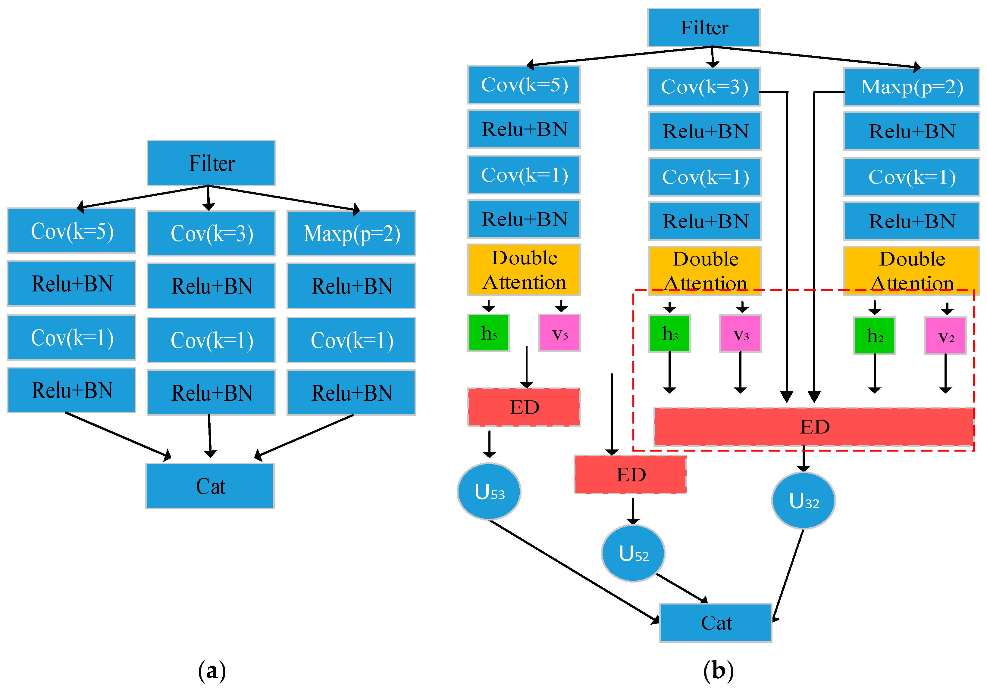
  • We use the Inception V3 [16] module and introduce multiple sets of Euclidean distance [17] strategies and bidirectional attention mechanism strategies to calculate the correlation between feature maps and feature points produced by kernel convolution at different scales at the same level. We select features based on the importance of each feature point.
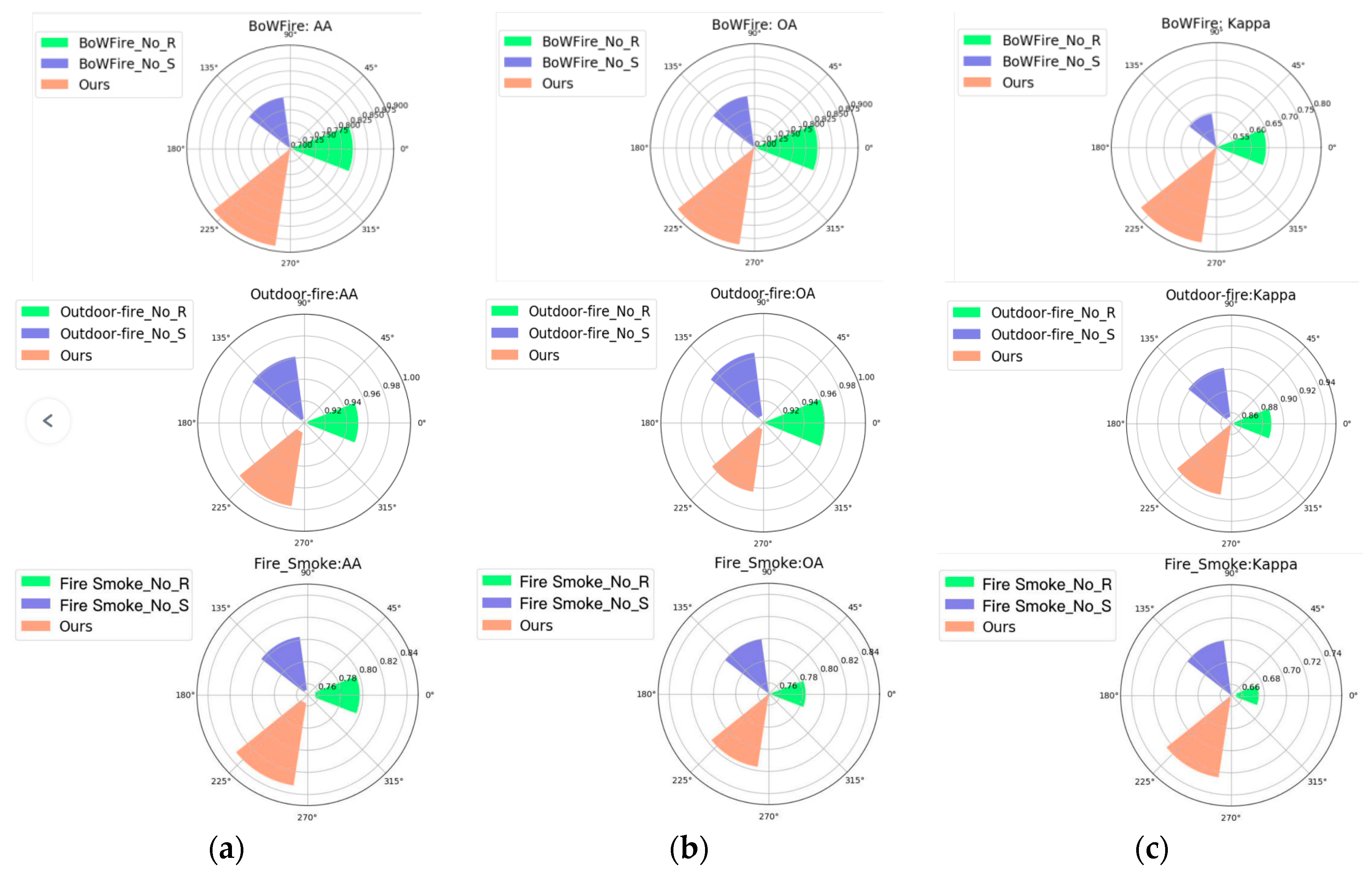
  • We conducted sufficient ablation experiments on three datasets to demonstrate the feasibility of the proposed strategy in this paper.
The main contents of the other sections in this paper are as follows. In the second section, we conduct further research and analyze the advantages and disadvantages of various network strategies for fire image classification. The third section introduces the relevant details of the BCFS-Net integration algorithm proposed in this paper. In the fourth section, we verify the comparison between the proposed BCFS-Net integration algorithm and other algorithms, as well as the practicality of various strategies in the BCFS-Net algorithm. The fifth section summarizes this paper.

2. Related Research

In recent years, deep learning has achieved certain results in fire detection tasks, and most models are based on convolution strategies or variants related to convolution in learning shallow features. Park M et al. [18] constructed a multitask transfer learning network for fire detection. Its hardcore algorithm is composed of VGG-16, ResNet-50, and DenseNet-121; learns the shallow features of data; and provides feature support for the MLC algorithm proposed in the latter stage. The results achieved the best effect on a set of open available multilabel classification task datasets. Liu Y et al. used AlexNet as the hardcore network of their algorithm to extract shallow features of smoke data. The relationship between the AlexNet submodules is strengthened through ResNet’s residual strategy. It provides feature points containing more semantic information for the final fully connected layer input by fully optimizing and learning shallow features. This algorithm achieves an accuracy of 98.56% on relevant fire and smoke datasets. Wang J. et al. [19] proposed a multichannel convolution strategy (DarkC-DCN), because multichannel convolution can obtain more abundant semantic information. Compared to the SENet module, convolution requires fewer computations than the fully connected layer, resulting in better performance. The results of this algorithm on multiple sets of fire datasets are 4.5% more accurate on average than those of multiple core networks. Compared with the latest algorithm, the DECA module proposed in its algorithm consumes fewer computational resources. Through the above research, we find that different convolution strategies can obtain different semantic information, thus further improving the quality of features. Other research on different convolution strategies, such as [20,21,22,23], has found that the existing research utilizes various strategies for learning and then fuses the feature maps generated by learning. Although more semantic information can be obtained, multiple modules or multichannel convolution will still generate a large number of calculation parameters.
Although shallow features contain rich semantic features, they still need to be further improved for the final task classification. Therefore, researchers need to further optimize the quality of each feature point. The attention mechanism assigns different weights to different feature points, which can help researchers further optimize the selection of shallow features. Yar H. et al. proposed a dual attention mechanism network for fire detection. The first attention mechanism of this algorithm is used in hardcore networks, which highlights important channels and generates efficient feature maps. The second attention mechanism of this algorithm is used to capture the spatial relationship between feature points and expand the differences between fire and no fire feature points. The proposed algorithm achieved the best results on four open datasets. Li S. et al. [24] proposed an accurate fire detection method. This method enhances the model’s learning ability for fire data through multiscale convolution and enhances the connections between feature maps through a dense skip link strategy. To further expand the differences between different channels, a new channel attention mechanism was constructed to emphasize the contributions between different feature maps. Hu Y. et al. [25] proposed an MVMNet algorithm. This algorithm uses YOLO5’s feature extractor to obtain shallow features. Subsequently, we construct a set of VAM modules to assign two sets of weights to each feature point and further highlight the feature points with significant weights through the strategy of adding weight values. Finally, fusing the new weights and feature points is the basis for the final classification. The algorithm has achieved good experimental results in both target detection and classification tasks for fires. Although the attention mechanism module can further expand the gap between different feature points, it only reduces the impact of lower-weighted feature points on the entire classification task and cannot completely constrain these feature points. Of course, attention mechanisms also play a positive role in other fire image tasks [26,27,28].
Through the above research, we found that fusing different convolution strategies can obtain richer semantic information. Second, through the attention mechanism, more attention can be given to fire characteristics, expanding the gap between fire areas and non-fire areas. Therefore, in this paper, we propose an integrated algorithm for bidirectional feature learning and deep feature selection. The core idea of this algorithm is to obtain more shallow features through bidirectional convolution of traditional convolution and dilated convolution. Then, the weight values of the same feature point with different discoveries are obtained through a bidirectional attention mechanism. The Euclidean distance strategy is used to filter out feature points with greater correction between the feature maps generated by each convolution in the Inception V3 module and preserve them to obtain more semantic information-rich feature points comprehensively considered and integrated from multiple dimensions. Finally, we use convolution to further learn the deep features and complete the final fire classification task.

3. BCFS-Net Algorithm

3.1. BCFS-Net Algorithm

We divided the BCFS-Net algorithm into three subparts. In the first part, we implemented data input and constructed a bidirectional feature learning module (DFM) to obtain shallow features generated by multiple sets of bidirectional traditional convolution and dilated convolution. In the second part, we used the weight selection module (WSM) and utilized the bidirectional attention mechanism and Euclidean distance to filter out feature points with greater correlation between the feature maps generated by each convolution layer in the Inception V3 module. Subsequently, multiple sets of weight coefficients generated by the cross-attention mechanism were combined with the Euclidean distance theorem to achieve the separation of useful and redundant features. In the third part, we used convolution fully connected layers to further learn and implement feature mapping for deep features and complete the final fire classification task. We constructed a model structure diagram of the BCFS-Net algorithm in Figure 1.

3.2. Bidirectional Feature Learning Module

The bidirectional feature learning module mainly obtains two sets of feature maps through traditional convolution and dilated convolution and obtains richer semantic information through different receptive fields. In this paper, the original input scale of the image is X R H W C , directly inputs X into traditional convolutions and dilated convolutions for feature learning, and Formulas (1) and (2) are expressed as follows. The process for obtaining local and global semantic information through multiscale convolution and multiscale dilated convolution is shown in Figure 2.
f T C = c o n v k = 5 , s = 2 ( m = 1 h n = 1 v ( x h , v w h , v + b h , v ) )
f A C = c o n v k = 5 d = 2 ( m = 1 h n = 1 v ( x h , v w h , v + b h , v ) )
f T C represents the operational results of traditional convolutions, f A C represents the operational results of dilated convolutions, x represents the characteristic points of the sample, h represents the horizontal coordinate axis, v represents the vertical coordinate axis, w represents the weight coefficient, b represents the bias function, k represents the size of the convolution kernel, d represents the scale of dilated convolution expansion, and s represents the step size of the convolution.
As Figure 2 shows, taking the convolution kernel equal to 3 and the step size equal to 1 as an example, traditional convolution and dilated convolution involve similar feature points during computation but can obtain different semantic information. Through two sets of convolutions, the DFM module obtains feature points with richer information, and we introduce a reverse convolution calculation. Formula (3) is as follows:
r T C = 0 f T C r A C = 0 f A C
r T C represents traditional convolution inverse feature points, and r A C represents dilated convolution inverse feature points. There are two reasons for this purpose. The first reason is that it can better reverse-highlight the importance of positive or negative sample feature points in feature maps. For example, when the values of feature points are 1, 0.5, and 0.2, the feature points with a value of 1 make the maximum contribution to the output layer. In contrast, when the feature point values become −1, −0.5, and −0.2, the feature point with a value of −0.2 makes the maximum contribution to the output layer. The second reason is that it is easier to distinguish between positive and negative feature points and perform targeted calculations. As shown in Formula (4), we perform separate addition operations on the positive and negative sample feature maps generated by traditional convolution and dilated convolution.
D F M f = f T C + f A C D F M r = r T C + r A C
D F M f represents the operational results of fusing positive sample feature points from traditional convolution and dilated convolution. Through the above calculations, we fused the positive sample feature points of traditional convolution and dilated convolution with each other, and at the same time, we fused the negative sample feature points of traditional convolution and dilated convolution with each other. To ensure the integrity of the image semantic information, we fused D F M f and D F M r using Formula (5). The output feature map F of the final shallow feature is obtained in step 1.
F = C a t ( D F M f , D F M r )

3.3. Weight Selection Module

The weight selection module consists of a bidirectional attention mechanism and a Euclidean distance strategy. In the WSM module, we first create two sets of attention mechanisms for the output of each submodule of the Inception V3 model and assign two sets of weight coefficients to each feature point. As shown in Formula (6), the Inception V3 module and the improved Inception V3 weight selection module are shown in Figure 3.
W k = 5 = F k = 5 , C h 5 , C v 5 W k = 3 = F k = 3 , C h 3 , C v 3 W p = 2 = F p = 2 , C h 2 , C v 2
F k = 5 , F k = 3 , F p = 2 represent the feature maps generated at different convolution kernel sales in the Inception V3 module separately, C h represent the weight coefficient of horizontal attention mechanism allocation, C v represent the weight coefficient of vertical attention mechanism allocation, and W k = 5 , W k = 3 , W p = 2 represent the feature map output of different convolution modules combined with bidirectional attention mechanisms in the Inception V3 module.
We add a bidirectional attention mechanism and Euclidean distance strategy to the Inception V3 module and introduce the output feature maps of the two submodules into the bidirectional attention mechanism and obtain the corresponding two sets of weight coefficients. Then, we introduce the two sets of weight coefficients and the original feature maps of the corresponding submodules into the Euclidean distance strategy and obtain the deep feature maps U . As shown in Formula (7), we obtain the similarity of each feature point between different submodules. Setting the threshold T , we preserve feature points with the same semantic information (positive and negative sample feature points) and rich semantic information expression between each submodule and keep them as a deep feature map. The detailed information is shown in Formula (8).
U 53 = E D ( W k = 5 , W k = 3 ) U 32 = E D ( W k = 3 , W k = 2 ) U 52 = E D ( W k = 5 , W k = 2 )
V = ( n 1 n 2 ) 2 + ( m 1 m 2 ) 2 Y U = θ ( V i , 1 ) , T V
Y U represents a new threshold weight matrix for deep features, θ represents the replacement function, V represents the matrix of Euclidean distance, n 1 and n 2 represent the horizontal weight coefficients of different submodules, and m 1 and m 2 represent the vertical weight coefficients of different submodules.
Finally, we describe the process of feature selection under the Euclidean distance strategy in Figure 4. When the T value is greater than the value V of the feature, we replace the value V with 1; otherwise, we replace V with 0. In the end, the point multiplication strategy of the matrix is used to achieve the direct replacement of the feature points.

3.4. Feature Dimension Reduction and Fusion

We obtain the final deep features after the weight selection of the module and integrate them through the convolution layer and fully connected layers. The specific Formula (9) is as follows:
C o v = C o v k = 1 ( C o v k = 3 ( M a x P o o l ( U ) ) ) F a l l = F l a t t e n ( C o n )
Cov represents the convolution, MaxPool represents the maximum pooling, and F a l l represents the reserved feature points before the classification of fire tasks.

4. Experimental Results

4.1. Datasets

In this paper, we validate our proposed BCFS-Net algorithm using three open available fire datasets. In this section, we will provide a detailed introduction to the three datasets.
BoWFire [29,30]: This dataset consists of 226 images, including 119 images with fire scenes (TB) and 107 images without fire scenes (Nor). The scale of each image in this dataset is 50 × 50 pixels. The data can be downloaded from the following website:
Outdoor Fire [31,32]: The dataset was created during the NASA Space Apps Challenge in 2018, and the goal was to use the dataset to develop a model that can recognize images with fire. The data are divided into two folders: the fire_images folder contains 755 outdoor fire images, some of which contain heavy smoke, and nonfire_images contain 244 natural images; it can be downloaded from the following website:
Fire Smoke [33,34]: This dataset consists of 1048 images, including 430 images with fire scenes, 457 images with smoke scenes, and 161 images without fire scenes. The data can be downloaded from the following website:
In this paper, we divided three sets of data into training, validation, and testing sets using the same random seeds for data partitioning. Their ratio was 7:1:2 (if the dataset contained the test data, we did not prepare the test dataset). Our server was a Tesla V100 16G, completed in the Keras deep learning environment. The learning rate was equal to 0.0001. The optimizer was Adam. The code we used was Python. All the following experiments were completed in a unified environment.

4.2. Evaluation Criteria

In this paper, we evaluate various models and ablation experiments using average accuracy (AA), overall accuracy (OA), and Kappa coefficients.
A A = 1 S ( n 1 m 1 + n 2 m 2 + + n S m S )
O A = n 1 + n 2 + + n S m 1 + m 2 + + m S
K a p p a = O A ( n 1 × m 1 + n 2 × m 2 + + n S × m S ) S × S 1 ( n 1 × m 1 + n 2 × m 2 + + n S × m S ) S × S
n 1 , n 2 , n 3 n S represent the number of samples in each category with correct prediction results. m 1 , m 2 , m 3 m S represent the original labels of each class sample. S represents the number of types of classes.
All experiments were conducted on the Tesla V100 32G server. All models in the experiment were performed with the Keras deep learning library and were written in Python. All algorithms used the Adam optimization function, and the learning rate was set to 0.0001. The binary cross-entropy loss function was used. Each training round had 64 samples. Each model was iterated 500 times.

4.3. Comparison between the BCFS-Net Algorithm and Other Algorithms

In this section, we compare the BCFS-Net algorithm with the hardcore algorithm and the latest algorithm. The results of each model in three sets of data are shown in Table 1, Table 2 and Table 3. The total parameter quantity and FLOPs (unit: M) of each model are shown in Table 4. We have bolded the optimal results for all experiments.
Table 1 shows that, on datasets with fewer samples, the improved algorithm is generally superior to the hardcore algorithm. EfficientNetB0 and DarkC-DCN have achieved significant good accuracy by constructing new convolution structures. The Inception-v3 network achieved better results than the other three sets of hardcore networks, indicating that the structure of Inception-v3 has a certain reference value. Both MVMNet and BCFS-Net in this paper introduced a bidirectional attention mechanism. The results indicated that the attention mechanism expands the differences between feature points, which greatly improves the prediction results. The BCFS-Net proposed in this paper has a higher OA value than the second-highest MVMNet by 2.4%. In terms of the AA value, it is 2.23% higher than the second-highest MVMNet, and in terms of the kappa value, it should be 4.4% higher than MVMNet. When there are fewer data samples, the effectiveness of Transformer and its improved algorithm is not significant, which may be due to the need for more data samples to support Transformer.
Table 2 shows that, as the number of data samples increases, the prediction accuracy of each model will be high, the new network structures such as EfficientNetB0 and MVMNet are slightly higher than hardcore networks, and ResNet50 and EfficientNetB0 both achieve good prediction results, possibly due to the residual strategy being more suitable for the outdoor fire dataset. When OA obtains the optimal value, the kappa coefficient of EfficientNetB0 is slightly higher than that of the BCFS-Net proposed in this paper. As shown in the threshold ablation experiment in Section 4.4, the kappa value of BCFS-Net also changes when the threshold setting is changed, with the optimal kappa value being 0.9163. From Table 2, we can see that the algorithm proposed in this paper has strong competitiveness in both overall accuracy and average accuracy. Transformer and TransFire also achieved good results in obtaining global semantic information on the outdoor fire dataset. Among them, TransFire’s kappa is optimal on the outdoor fire data, and the results show that, when the dataset sample size increases, Transformer’s global information learning is better.
From the experimental results in Table 3 above, it can be clearly seen that the BCFS-Net proposed in this paper still achieved the best results in multiclassification tasks, and the three sets of indicators were much higher than the other comparative models. This further indicates that the bidirectional feature learning module (DFM) and weight selection module (WSM) proposed in this paper have strong learning abilities on complex datasets.
Table 4 shows that the parameter quantity of the model proposed in this paper is relatively small and close to DenseNet121 and MVMNet. However, the results on the three datasets were much better than those of these two sets of models.

4.4. The Effect of Threshold T on BCFS-Net

The selection of deep features plays a decisive role in the final classification. The size of the Euclidean distance can directly indicate the similarity between the feature points corresponding to the convolution of each layer in the Inception V3 module. Different threshold settings directly affect the quantity and quality of deep feature retention. To further test the impact of different thresholds on each data point, we compare the results of the confusion matrix output by each model and the evaluation index.
Table 5 shows that, when the threshold is set to 0.5, all evaluation indicators achieve the optimal results. Figure 5 shows that, when the thresholds are set to 0.2 and 0.3, various results fluctuate greatly, affecting the prediction of fire and non-fire samples. When the thresholds are equal to 0.4 and 0.5, the prediction of various results is stable, and the accuracy of non-fire sample prediction reaches 90%.
Table 6 shows that, when the threshold is set to 0.4, OA achieves the optimal result of 0.9777, indicating that this threshold is more suitable for overall accuracy on the outdoor fire dataset. When the threshold is set to 0.3, AA achieves the optimal result of 0.9696 and a kappa coefficient of 0.9163, indicating that this threshold is more suitable for the average accuracy and comprehensive evaluation of the outdoor fire dataset. Figure 6 shows that, the smaller the threshold is, the more accurate the fire image detection accuracy. When the threshold is equal to 0.2, the fire image detection accuracy reaches 99%. When the threshold is equal to 0.4, the more accurate the detection of non-fire images reaches 1.
Table 7 shows that the optimal effect is achieved when the threshold is equal to 0.4. When the threshold is equal to 0.2 or 0.3, the results of the three sets of indicators are lower compared to T = 0.4, which is due to the retention of too many redundant feature points, resulting in a decrease in accuracy. From threshold 0.4 to threshold 0.6, we can see that the three sets of indicators gradually decrease due to the reduced selection of retained feature points and the loss of some features. In Figure 7, it is also easy to see that the TB and Nor accuracies gradually increase, and their accuracies are highest when the threshold is equal to 0.4; when the threshold is equal to 0.5, the Smoke class achieves the optimal result.

4.5. The Impact of Various Strategies on ResNet18 and Vgg16

To verify the applicability of the proposed strategy in this paper, we introduce a bidirectional feature learning module (DFM) and a weight selection module (WSM) into the ResNet18 network and the Vgg16 network. ResNet18 (DFM) represents the use of only bidirectional feature learning modules, and ResNet18 (WSM) represents the use of only weight selection modules. Vgg16(DFM) represents the use of only bidirectional feature learning modules, Vgg16(WSM) represents the use of only weight selection modules. The specific experimental results are shown in Table 8.
Table 8 shows that, in the BoWFire dataset, the results of DFM’s various indicators are more uniform than those of WSM, proving that DFM can better learn features from datasets with fewer samples. In the outdoor fire dataset, we can see that DFM has better OA metrics, while WSM has better kappa metrics, and both groups have better results than traditional ResNet18. On the Fire Smoke dataset, the experimental results of WSM were slightly better than those of DFM. The above experimental results for improving ResNet18 show that both sets of strategies proposed in this paper can increase the prediction accuracy of the model. By comparing the DFM and WSM bands in this article with Vgg16, it can be seen that DFM performs better. Similarly, on all three datasets, Vgg16 (DFM) and Vgg16 (WSM) outperformed Vgg16 in all indicators. From the improved Vgg16 algorithm, we further demonstrate that the DFM and WSM strategies proposed in this paper are feasible.

4.6. Feasibility of Various Strategies in the BCFS-Net Algorithm

Different strategies learn different semantic information of images. The shallow and deep features retained simultaneously are also different. To further test whether the proposed strategy has a learning ability on three sets of open datasets, this section discusses the two sets of strategies proposed in the BCFS-Net algorithm. To conveniently obtain the advantages and disadvantages of the strategy proposed in this paper, this section uses a polar pie chart (Figure 8) and the loss function of the training process (Figure 9). The visualization results on specific datasets are shown in Figure 8. Among them, “No_R” indicates that the BCFS-Net algorithm does not use a bidirectional feature learning module, and “No_S” indicates that the BCFS-Net algorithm does not use a weight selection module.
From the first set of polar pie charts in Figure 8, it can be seen that using a weight selection module is more effective than using a bidirectional feature learning module. The results of the polar pie chart presented in the outdoor fire dataset indicate that both strategies have similar feature learning abilities and that both have certain learning abilities. In the third dataset, the bidirectional feature learning module is superior to the weight selection module. From the above three sets of polar pie charts, it can be seen that the two strategies proposed in this paper work best when used together. Therefore, this further proves the importance of the model for feature learning and feature selection.
From Figure 9, it can be seen that, when the BCFS-Net model uses the bidirectional feature learning module and weight selection module, the loss performance is lower. However, due to the large and relatively simple number of data samples in the outdoor fire dataset, there is not much difference in the training process between using two sets of strategies. However, the Fire Smoke dataset is the most complex, with significant loss differences when both BCFS-Net modules are used. The training process loss can indicate that the strategy proposed in this article performs better compared to complex data.

5. Summary and Outlook

We propose a new deep learning algorithm, BCFS-Net, in this paper. The main task of this algorithm is to obtain richer shallow features through bidirectional feature learning modules and then use the weight selection module to filter deep features. This algorithm proves that the BCFS-Net algorithm can be better suited for fire image classification tasks on three datasets. In the deep features, we preserve semantically rich feature points, but it will lose some semantic information. Therefore, in the next step, we will relearn the lost features and obtain some semantic features to fuse with the retained deep features. Through this method, we will further improve the detection accuracy of the algorithm for fire image classification tasks.

Author Contributions

Z.W. is responsible for the writing of the paper, method design, and experimental training. X.Z. and Y.T. participated in the review. All authors have read and agreed to the published version of the manuscript.

Funding

This research was supported by the Fundamental Research Funds for the Central Universities (No. 2020ZDPY0223).

Data Availability Statement

The data presented in this study are available on request from the corresponding author The data are not publicly available due to privacy reasons.

Acknowledgments

We are very grateful to my peers for their support and to the reviewers who gave constructive comments.

Conflicts of Interest

The authors declare no conflict of interest.

References

  1. Khudayberdiev, O.; Zhang, J.; Elkhalil, A.; Balde, L. Fire detection approach based on vision transformer. In Proceedings of the International Conference on Adaptive and Intelligent Systems, Larnaca, Cyprus, 25–26 May 2022; Springer International Publishing: Cham, Switzerland, 2022; pp. 41–53. [Google Scholar]
  2. Ghali, R.; Akhloufi, M.A.; Mseddi, W.S. Deep learning and transformer approaches for UAV-based wildfire detection and segmentation. Sensors 2022, 22, 1977. [Google Scholar] [CrossRef] [PubMed]
  3. Ayala, A.; Fernandes, B.; Cruz, F.; Macêdo, D.; Oliveira, A.L.; Zanchettin, C. KutralNet: A portable deep learning model for fire recognition. In Proceedings of the 2020 International Joint Conference on Neural Networks (IJCNN), Glasgow, UK, 19–24 July 2020; pp. 1–8. [Google Scholar]
  4. Majid, S.; Alenezi, F.; Masood, S.; Ahmad, M.; Gündüz, E.S.; Polat, K. Attention based CNN model for fire detection and localization in real-world images. Expert Syst. Appl. 2022, 189, 116114. [Google Scholar] [CrossRef]
  5. Zhang, J.; Zhu, H.; Wang, P.; Ling, X. ATT squeeze U-Net: A lightweight network for forest fire detection and recognition. IEEE Access 2021, 9, 10858–10870. [Google Scholar] [CrossRef]
  6. Tripathi, A.M.; Mishra, A. Environment sound classification using an attention-based residual neural network. Neurocomputing 2021, 460, 409–423. [Google Scholar] [CrossRef]
  7. Lin, J.; Lin, H.; Wang, F. A Semi-Supervised Method for Real-Time Forest Fire Detection Algorithm Based on Adaptively Spatial Feature Fusion. Forests 2023, 14, 361. [Google Scholar] [CrossRef]
  8. Xue, Z.; Lin, H.; Wang, F. A small target forest fire detection model based on YOLOv5 improvement. Forests 2022, 13, 1332. [Google Scholar] [CrossRef]
  9. Ning, X.; Tian, W.; He, F.; Bai, X.; Sun, L.; Li, W. Hypersausage coverage function neuron model and learning algorithm for image classi cation. Pattern Recognit. 2023, 136, 109216. [Google Scholar] [CrossRef]
  10. Ning, X.; Tian, W.; Yu, Z.; Li, W.; Bai, X.; Wang, Y. HCFNN: High-order Coverage Function Neural Network for Image Classification. Pattern Recognit. 2022, 131, 108873. [Google Scholar] [CrossRef]
  11. Wang, Z.; Zhang, T.; Wu, X.; Huang, X. Predicting transient building fire based on external smoke images and deep learning. J. Build. Eng. 2022, 47, 103823. [Google Scholar] [CrossRef]
  12. Ning, X.; Yu, Z.; Li, L.; Li, W.; Tiwari, P. Differentiable rendering-based multiview Image-Language Fusion for zero-shot 3D shape understanding. Inf. Fusion 2023, 102, 102033. [Google Scholar] [CrossRef]
  13. Harkat, H.; Nascimento, J.M.; Bernardino, A.; Ahmed, H.F.T. Fire images classification based on a handcraft approach. Expert Syst. Appl. 2023, 212, 118594. [Google Scholar] [CrossRef]
  14. Liu, Y.; Qin, W.; Liu, K.; Zhang, F.; Xiao, Z. A dual convolution network using dark channel prior for image smoke classification. IEEE Access 2019, 7, 60697–60706. [Google Scholar] [CrossRef]
  15. Yar, H.; Hussain, T.; Agarwal, M.; Khan, Z.A.; Gupta, S.K.; Baik, S.W. Optimized dual fire attention network and medium-scale fire classification benchmark. IEEE Trans. Image Process. 2022, 31, 6331–6343. [Google Scholar] [CrossRef] [PubMed]
  16. You, H.; Yu, L.; Tian, S.; Cai, W. A stereo spatial decoupling network for medical image classification. Complex Intell. Syst. 2023, 9, 5965–5974. [Google Scholar] [CrossRef] [PubMed]
  17. Huang, C.; Su, B.-C.; Lin, T.; Huang, Y. Downlink SCMA codebook design with low error rate by maximizing minimum Euclidean distance of superimposed codewords. IEEE Trans. Veh. Technol. 2022, 71, 5231–5245. [Google Scholar] [CrossRef]
  18. Park, M.; Tran, D.Q.; Lee, S.; Park, S. Multilabel image classification with deep transfer learning for decision support on wildfire response. Remote Sens. 2021, 13, 3985. [Google Scholar] [CrossRef]
  19. Wang, J.; Yu, J.; He, Z. DECA: A novel multiscale efficient channel attention module for object detection in real-life fire images. Appl. Intell. 2022, 52, 1362–1375. [Google Scholar] [CrossRef]
  20. Sarıgül, M.; Ozyildirim, B.M.; Avci, M. Differential convolutional neural network. Neural Netw. 2019, 116, 279–287. [Google Scholar] [CrossRef] [PubMed]
  21. Ahmad, I.; Pothuganti, K. Analysis of different convolution neural network models to diagnose Alzheimer’s disease. Mater. Today Proc. 2020. [Google Scholar] [CrossRef]
  22. Uyulan, C.; Ergüzel, T.T.; Unubol, H.; Cebi, M.; Sayar, G.H.; Asad, M.N.; Tarhan, N. Major depressive disorder classification based on different convolutional neural network models: Deep learning approach. Clin. EEG Neurosci. 2021, 52, 38–51. [Google Scholar] [CrossRef]
  23. Nanni, L.; Brahnam, S.; Paci, M.; Ghidoni, S. Comparison of Different Convolutional Neural Network Activation Functions and Methods for Building Ensembles for Small to Midsize Medical DataSets. Sensors 2022, 22, 6129. [Google Scholar] [CrossRef] [PubMed]
  24. Li, S.; Yan, Q.; Liu, P. An efficient fire detection method based on multiscale feature extraction, implicit deep supervision and channel attention mechanism. IEEE Trans. Image Process. 2020, 29, 8467–8475. [Google Scholar] [CrossRef] [PubMed]
  25. Hu, Y.; Zhan, J.; Zhou, G.; Chen, A.; Cai, W.; Guo, K.; Hu, Y.; Li, L. Fast forest fire smoke detection using MVMNet. Knowl.-Based Syst. 2022, 241, 108219. [Google Scholar] [CrossRef]
  26. Anderson, E.B.; Mitchell, J.F.; Reynol DRSFJ, H. Attentional modulation of firing rate varies with burstiness across putative pyramidal neurons in macaque visual area V4. J. Neurosci. 2011, 31, 10983–10992. [Google Scholar] [CrossRef] [PubMed]
  27. Cannon, J.B.; Peterson, C.J.; O’Brien, J.J.; Brewer, J.S. A review and classification of interactions between forest disturbance from wind and fire. For. Ecol. Manag. 2017, 406, 381–390. [Google Scholar] [CrossRef]
  28. Yu, Y.; Fu, L.; Cheng, Y.; Ye, Q. Multiview distance metric learning via independent and shared feature subspace with applications to face and forest fire recognition, and remote sensing classification. Knowl.-Based Syst. 2022, 243, 108350. [Google Scholar] [CrossRef]
  29. Chino, D.Y.; Avalhais, L.P.; Rodrigues, J.F.; Traina, A.J. Bowfire: Detection of fire in still images by integrating pixel color and texture analysis. In Proceedings of the 2015 28th SIBGRAPI Conference on Graphics, Patterns and Images, Washington, DC, USA, 26–29 August 2015; pp. 95–102. [Google Scholar]
  30. Mlích, J.; Koplík, K.; Hradiš, M.; Zemčík, P. Fire segmentation in still images. In Proceedings of the Advanced Concepts for Intelligent Vision Systems: 20th International Conference, ACIVS 2020, Auckland, New Zealand, 10–14 February 2020; Proceedings 20. Springer International Publishing: Cham, Switzerland, 2020; pp. 27–37. [Google Scholar]
  31. Saponara, S.; Elhanashi, A.; Gagliardi, A. Real-time video fire/smoke detection based on CNN in antifire surveillance systems. J. Real-Time Image Process. 2021, 18, 889–900. [Google Scholar] [CrossRef]
  32. Shi, L.; Long, F.; Lin, C.; Zhao, Y. Video-based fire detection with saliency detection and convolutional neural networks. In Advances in Neural Networks-ISNN 2017: 14th International Symposium, ISNN 2017, Sapporo, Hakodate, and Muroran, Hokkaido, Japan, 21–26 June 2017, Proceedings, Part II 14; Springer International Publishing: Cham, Switzerland, 2017; pp. 299–309. [Google Scholar]
  33. Dewangan, A.; Pande, Y.; Braun, H.-W.; Vernon, F.; Perez, I.; Altintas, I.; Cottrell, G.W.; Nguyen, M.H. FIgLib & SmokeyNet: Dataset and deep learning model for real-time wildland fire smoke detection. Remote Sens. 2022, 14, 1007. [Google Scholar]
  34. Zhang, Q.-X.; Lin, G.-H.; Zhang, Y.-M.; Xu, G.; Wang, J.-J. Wildland forest fire smoke detection based on faster R-CNN using synthetic smoke images. Procedia Eng. 2018, 211, 441–446. [Google Scholar] [CrossRef]
  35. Sathishkumar, V.E.; Cho, J.; Subramanian, M.; Naren, O.S. Forest fire and smoke detection using deep learning-based learning without forgetting. Fire Ecol. 2023, 19, 9. [Google Scholar] [CrossRef]
  36. Alqahtani, M.M.; Dutta, A.K.; Almotairi, S.; Ilayaraja, M.; Albraikan, A.A.; Al-Wesabi, F.N.; Al Duhayyim, M. Sailfish Optimizer with EfficientNet Model for Apple Leaf Disease Detection. Comput. Mater. Contin. 2023, 75, 217–233. [Google Scholar]
  37. Ghali, R.; Akhloufi, M.A. Deep Learning Approaches for Wildland Fires Remote Sensing: Classification, Detection, and Segmentation. Remote Sens. 2023, 15, 1821. [Google Scholar] [CrossRef]
  38. Akyol, K. A comprehensive comparison study of traditional classifiers and deep neural networks for forest fire detection. Clust. Comput. 2023, 1–15. [Google Scholar] [CrossRef]
Figure 1. BCFS-Net algorithm overall structure diagram, Electronics 12 04566 i001 represents the vertical weight coefficients for obtaining feature maps (v), and Electronics 12 04566 i002 represents the lateral weight coefficients for obtaining feature maps. ED represents the operational strategy of the Euclidean theorem. Electronics 12 04566 i003 representing the feature points retained after Euclidean distance filtering.
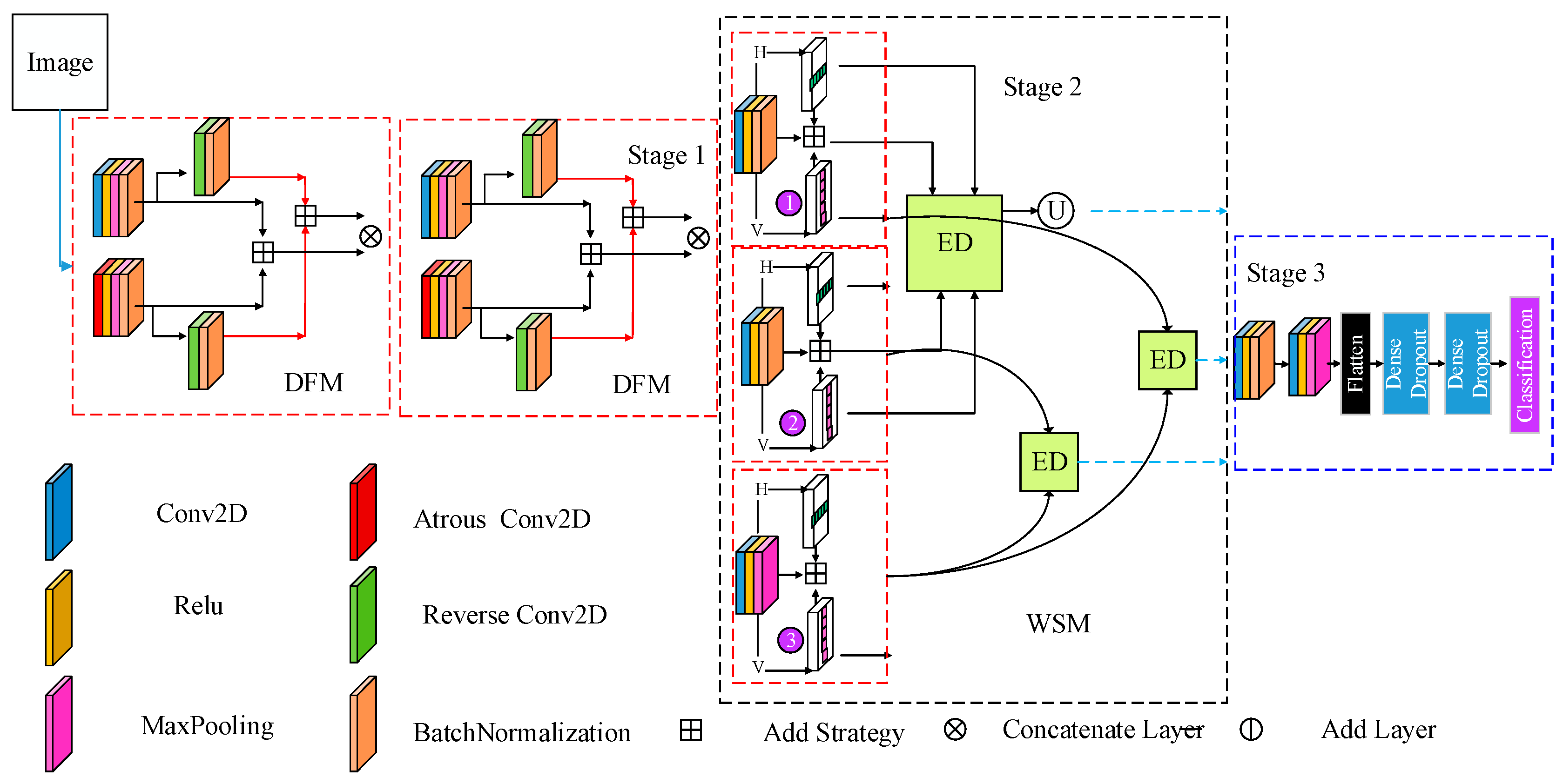
Electronics 12 04566 g001
Figure 2. (a) Shallow features obtained by traditional convolution; (b) shallow features obtained by dilated convolution. The blue circle represents the feature points obtained after the convolution operation. The red and blue circles represent the feature points participating in the calculation. The light blue circles do not participate. The green circles represent another set of feature points that participate in the calculation.
Electronics 12 04566 g002
Figure 3. (a) Inception V3 module; (b) weight selection module.
Electronics 12 04566 g003
Figure 4. Process of feature selection based on the Euclidean distance strategy. In the above figure, n and m represent the weight coefficients in both directions, U represents the output of useful features, R represents the output of redundant features (the semantic information with fewer feature points will be directly eliminated), ED represents the Euclidean distance strategy, and dots represent the feature map and the new threshold weight matrix point multiplication strategy. T represents the threshold. 1 and 0 represent the matrix of all 1 and all 0. The black dashed box represents the threshold screening process.
Electronics 12 04566 g004
Figure 5. The results of setting different thresholds on the BoWFire dataset. TB represents the fire data sample, and Nor represents the non-fire data sample. (a) T = 0.2; (b) T = 0.3; (c) T = 0.4; (d) T = 0.5; (e) T = 0.6.
Electronics 12 04566 g005
Figure 6. The results of setting different thresholds on the outdoor fire dataset. TB represents the fire data sample, and Nor represents the non-fire data sample. (a) T = 0.2; (b) T = 0.3; (c) T = 0.4; (d) T = 0.5; (e) T = 0.6.
Electronics 12 04566 g006
Figure 7. The results of setting different thresholds on the Fire Smoke dataset. TB represents the fire data sample, and Nor represents the non-fire data sample. (a) T = 0.2; (b) T = 0.3; (c) T = 0.4; (d) T = 0.5; (e) T = 0.6.
Electronics 12 04566 g007
Figure 8. The impact of each strategy on different datasets. The first row contains three sets of indicators from the BoWFire dataset, the second row contains three sets of indicators for the outdoor fire dataset, and the third row contains three sets of metrics for the Fire Smoke dataset. (a) AA value; (b) OA value; (c) kappa value.
Electronics 12 04566 g008
Figure 9. Loss of training process for different strategies on different datasets. (a) BoWFire dataset; (b) outdoor fire dataset; (c) Fire Smoke dataset. Calculate the average loss every 20 iterations.
Electronics 12 04566 g009
Table 1. Classification results of each model on the BoWFire dataset.
ModelBoWFire Dataset
OAAAKappa
VGG16 [35]0.81270.80000.6041
DenseNet121 [36]0.82310.82220.6449
ResNet50 [37]0.75000.7330.4545
Xception [38]0.73410.73330.4674
InceptionV30.83000.82200.6470
EfficientNetB00.84820.84440.6902
MVMNet0.86600.86660.7321
DarkC-DCN0.85180.84440.6846
BCFS-Net0.89000.88890.7761
Transformer [1]0.83520.82440.6535
TransFire [2]0.84370.84330.6839
BCFS-Net0.89000.88890.7761
Table 2. Classification results of each model on the outdoor fire dataset.
ModelOutdoor Fire Dataset
OAAAKappa
VGG16 [35]0.90390.92420.7890
DenseNet121 [36]0.94080.95450.8753
ResNet50 [37]0.94500.95900.8900
Xception [38]0.93550.95450.8771
InceptionV30.93090.95450.8788
EfficientNetB00.95480.96460.9030
MVMNet0.95410.95450.8717
DarkC-DCN0.94700.95450.8735
BCFS-Net0.97770.96460.8987
Transformer [1]0.94630.95450.8722
TransFire [2]0.95720.96460.9041
BCFS-Net0.97770.96460.8987
Table 3. Classification results of each model on the Fire Smoke dataset.
ModelFire Smoke Dataset
OAAAKappa
VGG16 [35]0.68700.68600.5300
DenseNet121 [36]0.75330.75000.6250
ResNet50 [37]0.76660.76660.6500
Xception [38]0.71330.71330.5700
InceptionV30.78400.75600.6350
EfficientNetB00.77350.77330.6600
MVMNet0.78070.76000.6400
DarkC-DCN0.78420.77660.6650
BCFS-Net0.83280.81660.7250
Transformer [1]0.75460.74970.6200
TransFire [2]0.76320.76000.6350
BCFS-Net0.83280.81660.7250
Table 4. Total parameter quantity and FLOPs of each model.
ModelFire Smoke Dataset
ParamsFLOPs
VGG1629.53 M14.82 M
DenseNet12114.78 M7.16 M
ResNet5047.41 M23.58 M
Xception42.54 M21.12 M
InceptionV344.10 M21.94 M
EfficientNetB031.49 M15.73 M
MVMNet14.78 M7.24 M
DarkC-DCN106.22 M53.06 M
Transformer199.12 M99.03 M
TransFire217.53 M103.38 M
BCFS-Net14.50 M7.24 M
Table 5. Classification results of different thresholds on the BoWFire dataset.
ModelBoWFire Dataset
OAAAKappa
BCFS-Net (T = 0.6)0.84500.84440.8650
BCFS-Net (T = 0.5)0.89000.88890.7761
BCFS-Net (T = 0.4)0.86600.86660.7321
BCFS-Net (T = 0.3)0.84380.84440.6880
BCFS-Net (T = 0.2)0.82310.82220.6449
Table 6. Classification results of different thresholds on the outdoor fire dataset.
ModelOutdoor Fire Dataset
OAAAKappa
BCFS-Net (T = 0.6)0.94500.95950.8900
BCFS-Net (T = 0.5)0.96140.96460.9017
BCFS-Net (T = 0.4)0.97770.96460.8987
BCFS-Net (T = 0.3)0.96500.96960.9163
BCFS-Net (T = 0.2)0.95320.95320.9186
Table 7. Classification results of different thresholds on the Fire Smoke dataset.
ModelFire Smoke Dataset
OAAAKappa
BCFS-Net (T = 0.6)0.79450.79000.6850
BCFS-Net (T = 0.5)0.81030.80670.7100
BCFS-Net (T = 0.4)0.83280.81660.7250
BCFS-Net (T = 0.3)0.78420.78330.6750
BCFS-Net (T = 0.2)0.79900.79900.6950
Table 8. The classification results of the ResNet18 network in three datasets using various strategies.
ModelBoWFire DatasetOutdoor Fire DatasetFire Smoke Dataset
OAAAKappaOAAAKappaOAAAKappa
RseNet180.82140.82220.64280.9450.95950.89000.73500.72660.5900
RseNet18 (DFM)0.84820.84440.69020.96140.96460.90160.75360.74330.6150
RseNet18 (WSM)0.83000.82220.64700.94910.96460.90440.75010.75330.6300
Vgg160.81270.80000.60410.90390.92420.78900.68700.68600.5300
Vgg16 (DFM)0.83710.83330.65830.93420.95450.88210.73440.75330.6350
Vgg16 (WSM)0.82930.82220.64260.92110.95450.87610.71350.72260.5850
Disclaimer/Publisher’s Note: The statements, opinions and data contained in all publications are solely those of the individual author(s) and contributor(s) and not of MDPI and/or the editor(s). MDPI and/or the editor(s) disclaim responsibility for any injury to people or property resulting from any ideas, methods, instructions or products referred to in the content.

