Comparison of Coverage-Prediction Models for Modern Mobile Radio Networks

Abstract

The accurate prediction of a signal’s attenuation is essential for the development of reliable, modern, mobile radio-communication networks. In this study, the accuracies of four propagation models in diverse terrains and environments were analyzed using field measurements along a comprehensive test route. We evaluated the ability of the models—Egli, Okumura, Hata–Davidson, and Longley–Rice—to predict signal propagation in the Very-High-Frequency (VHF) and Ultra-High-Frequency (UHF) bands. Based on a meticulous comparison, we present valuable insights into the strengths and limitations of these models, enhancing coverage-prediction methodologies for evolving mobile radio networks. The Egli model, despite its simplicity, introduces significant inaccuracies due to its assumptions and a lack of consideration for the terrain. The Okumura model, which is widely used in urban areas, requires careful correction selection, while the Hata–Davidson model improves upon the former’s weaknesses. The Longley–Rice model excels in flexibility and accuracy, especially in the VHF bands, using topographical data, though it can overestimate the attenuation in shadowed areas. The study concluded that no single model was universally accurate, as each model has its strengths and limitations. It highlights the need for informed model selection based on the terrain’s characteristics and specific requirements. The results will be useful to network planners, helping them to design efficient, mobile communication networks with reliable coverage and optimal spectrum utilization. The Longley–Rice model emerged as particularly powerful, offering detailed predictions across diverse environments.

1. Introduction

In an era marked by the relentless pursuit of seamless connectivity, advanced mobile networks are the foundation of our increasingly digitized world—on its way to the metaverse [1]. These networks, from 5G to the emerging 6G and beyond, have undergone a remarkable transformation to meet the ever-growing demands for high-speed data, low latency, and ubiquitous coverage [2,3]. Ensuring reliable and efficient coverage in diverse landscapes, urban environments, and emerging use cases remains one of the biggest challenges in mobile communications [4,5]. In this context, the analysis of various propagation models assumes significance, as it influences network planning, optimization, and spectrum-allocation decisions.

The field of radio-wave propagation modeling has seen extensive research and development over the years [4,5]. Earlier models, such as the Egli model, laid the groundwork for predicting path loss. However, their simplicity often led to inaccuracies, particularly in complex terrains and urban environments [6]. Subsequent models, like the Okumura model, incorporated empirical adjustments based on real-world measurements in urban areas [7]. Nevertheless, discrepancies arise when applying such models to diverse terrains due to the inherent assumptions and limited correction factors.

Controversies emerge in the realm of model selection, as different models exhibit strengths in specific scenarios. While the Okumura model is recognized for its accuracy in urban contexts, the Hata–Davidson model introduces additional adjustments that attempt to address the shortcomings of earlier models [8]. Moreover, the Longley–Rice model stands out for its flexibility. It uses topographic data and probabilistic considerations to provide comprehensive predictions [9]. However, as with any model, its complexity and limitations in specific scenarios should be considered when selecting a propagation model for particular applications.

The objective of this article is to evaluate the effectiveness of four commonly used propagation models—the Egli model, the Okumura model, the Hata–Davidson model, and the Longley–Rice model—in predicting signal propagation in the Very-High-Frequency (VHF) and Ultra-High-Frequency (UHF) bands, which cover frequencies from 30 MHz to 3 GHz. These four models were selected due to their widespread use as empirical models for path-loss prediction in the VHF and UHF bands [10]. They serve as fundamental tools for estimating the path loss and radio-signal coverage across diverse terrains and environments. A comprehensive understanding of their strengths and limitations is crucial for making well-informed decisions about the design of wireless networks.

When planning VHF and UHF networks, we concluded that the calculations of the individual models do not reflect the real situation in the field. Sometimes, these deviations are so large that the constructed network of repeaters has larger “gaps”, where the coverage is insufficient and communication is not possible. The need for additional repeaters makes network construction more expensive, and users receive poor service. Therefore, we decided to empirically, with field measurements, check the four most-used models: Egli, Okumura, Hata–Davidson, and Longley–Rice.

The principal aim of this work is to provide network planners, researchers, and practitioners with a comprehensive understanding of the performance characteristics of these propagation models. By highlighting their strengths and limitations, we aim to guide the selection of appropriate models based on the specific environment of interest. Ultimately, our study contributes to the optimization of communication networks, ensuring reliable coverage and efficient spectrum utilization.

The rest of the article is organized as follows. In the next section, we present the basic principles of the computational algorithms for the prediction models and methods. This is followed by a description of the measurement equipment and the 40 km route used for the field measurements and a thorough comparison of the prediction capabilities of the four propagation models based on an analysis of the field measurements made along a diverse test route. We evaluate their accuracy in rural, suburban, and urban areas by considering varying terrain ruggedness and obstruction patterns. By examining the deviations between the models’ predictions and the actual field measurements, we gain insights into their suitability for different scenarios. In summary, the conclusions of this study provide an assessment of widely used propagation models in the context of radio-wave propagation prediction. By examining their accuracy and deviations in various terrains and scenarios, we aim to facilitate informed decision making in wireless-network design and optimization. The details are presented in the conclusion, and our basic findings are outlined below:

• Certain models give much more accurate results than others;
• Corrections built into the models for the type of terrain (open, quasi-open, suburban, urban) do not always improve the accuracy of the prediction;
• The accuracy of the prediction requires an experienced engineer to apply the appropriate correction.

2. Prediction Models and Methods

2.1. Analyzed Models

We analyzed four commonly used models for predicting the propagation of electromagnetic waves in the VHF (30 to 300 MHz) and UHF (300 to 3 GHz) bands. As these are well-established and well-known models, only their summaries are provided along with the fundamental principles of their computational algorithms.

2.1.1. Egli Model

The first model included in the study is the Egli model. This is a basic and highly simplified model that does not consider the actual terrain relief but assumes a relief similar to the Earth’s plane with an average roughness of approximately 15 m [6]. As a result, the propagation attenuation is only adapted to the height of the transmitting and receiving antennas. The Egli model is considered a pioneer in predicting the path loss between two points. The model is based on a series of measurements on predominantly flat terrain over a wide frequency range from 90 MHz to 1 GHz [7]. For the prediction, the Egli model uses the basic attenuation shown in Equation (1) with the addition of a β factor, which can be calculated according to Equation (2)

$$L_E=G_{TX}{G}_{RX}{\left(\frac{h_{TX}{h}_{RX}}{d^2}\right)}^2\beta$$

(1)

$$\beta ={\left(\frac{40}{f}\right)}^2$$

(2)

where G_TX and G_RX are the gains of the transmitting and receiving antenna, and h_TX and h_RX are the heights of the transmitting and receiving antennas. The β factor is obtained from empirical measurements and is frequency dependent.

Egli’s model assumes that there is always a line-of-sight between the transmitter and the receiver. A weakness of the model is the definition of rugged terrain, which is derived entirely empirically and does not account for diffraction losses. Consequently, the method has limitations for use in areas with more rugged terrain or large obstacles. Nevertheless, the model later introduces a widely used factor of a log-normal probability distribution of the link losses within the signal propagation area [6,7].

2.1.2. Okumura Model

The Okumura method is a widely used empirical method for predicting signal attenuation that was developed primarily for populated urban areas. It is based on an extensive series of measurements in Tokyo up to a frequency of 1920 MHz [7,8]. This model calculates the basic median field strength and then adjusts it based on factors such as the ruggedness of the terrain, urbanization level (Urban Large, Urban Medium, Suburban, Quasi-Open, and Open), terrain slope, etc.

A series of correction factors are added to the free-space attenuation equation (F_SP) so that the attenuation equation of the Okumura–Hata method is

$$L=L_{FS}+L_{mu}+H_{TX}+H_{RX}+K_a-K_A.$$

(3)

L_mu is the median attenuation with respect to empty space in an urban area over almost flat land with an effective height of the transmitting antenna h_TXe = 200 m and a reference height of the receiving antenna h_RXe = 3 m. The corrections H_TX for the transmitting antenna and H_RX for the receiving antenna are used for antenna heights that are not at the reference heights. K_a is the street-orientation-correction factor. This takes into account the attenuation correction based on the relationship between the direction of movement of the receiver (e.g., in a vehicle) and the direction of propagation of the radio signal. K_A is a correction for a suburban, rural or open area.

Over time, the Okumura method has seen a lot of upgrades and enhancements. Therefore, it is considered as one of the most established models for predicting attenuation, and it is often used as a standard for comparing other methods [7,8]. The method has a wide range of applications; however, its use is limited to those ranges of parameters that are defined by measured or calculated curves and their extrapolation. Additionally, in some cases, simple interpolation might not be realistic, requiring a careful evaluation of the results. The major weakness of the method is the classification of the analyzed area because the urban area of Tokyo, where the method was developed, can differ from European urban areas.

2.1.3. Hata–Davidson Model

The Hata–Davidson model is based on the previously described Okumura model. In fact, it is an extension of Okumura with several empirical curves to determine the adjustment factors. The calculation of the basic median field strength is slightly different and does not consider the topography along the entire path between the transmitter and the receiver.

To make Okumura’s graphical methods easier to use, Hata introduced some empirical mathematical formulas. However, Hata’s formulations are limited to strictly defined ranges of input values and are intended for use only in nearly flat terrain with Δh < 20 m [6,7].

The model does not include the entire set of Okumura’s corrections; nevertheless, the results of the model are expected to match relatively well with field measurements. This method might slightly lean toward generalizing certain extreme situations, as it responds too slowly to rapid changes in the radio signal’s propagation-path profile. Generally, the prediction technique is considered to be very successful in urban and suburban areas and somewhat less accurate in rural and rugged terrain [7,8].

2.1.4. Longley–Rice Model

One of the most popular models for predicting field strength, especially in the VHF and UHF bands, is the Longley–Rice model, which is also known as the Irregular Terrain Model (ITM). It is considered as a widely applicable and highly flexible prediction model.

The Longley–Rice model is a very advanced model for predicting attenuation with broad usability. This model allows adjustments for different climates and incorporates a variable assessment of the probability of link loss over time and locations based on the calculated median path loss [7]. One of the features of this method is that a correction for the urban environment is introduced to calculate the attenuation in urban environments.

$$UF=16.5+15{\mathit{log}}_{10}\left(\frac{f}{100}\right)-0.12d$$

(4)

where the frequency f is given in MHz and the distance d is given in kilometers. The UF is expressed in decibels.

Its main limitation is that except for the correction factor in urban areas (Urban Factor, UF), it does not consider any variables related to the potential proximity to obstacles like buildings or vegetation near the transmitter or receiver [7,9].

2.2. Measurement Equipment

For the purposes of computer calculations and field measurements with subsequent analysis, several computer programs and dedicated items of radio equipment were used. All the computer calculations were performed using TAP 7.5 software by SoftWright (www.softwright.com). The TAP Mapper 7.5 program was used for a visualization and analysis of the calculated coverage as well as for comparing the calculated and on-site measured data and their visualization.

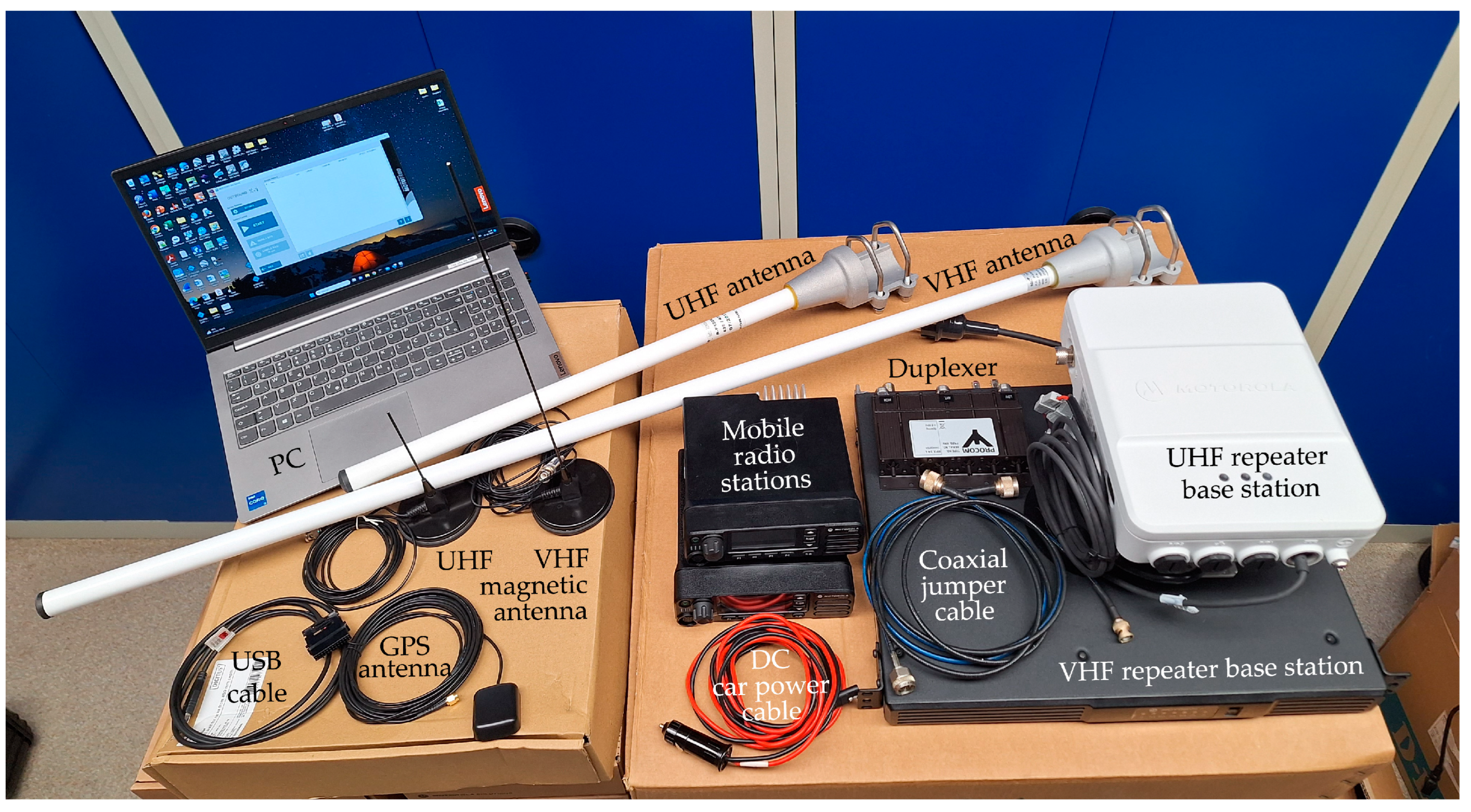
The repeater base-station for the field measurements was in Slovenia on a small hill above Ljubljana. The VHF radio equipment consisted of a Motorola SLR 5500 repeater base-station with a Procom MPX2/6H antenna duplexer and a R-F 133 NH vertical half-wave dipole antenna with a 0 dBd gain, which was mounted on an 8 m radio tower. The UHF radio equipment included a Motorola SLR 1000 repeater base-station with a HKFE4004A antenna duplexer and an R-F 130 NZ vertical half-wave dipole antenna with a 0 dBd gain, which was mounted on the same 8 m radio tower.

The receiving radio stations were VHF and UHF Motorola DM4601e mobile radios with tuned quarter-wave vertical antennas Nagoya UT-308UV with 0 dBd gain and active Global Positioning System (GPS) antenna DAM 1575A2. The mobile radios with antennas were installed in a vehicle, enabling field measurements along a pre-defined test route.

In the VHF frequency range, the repeater was transmitting on 173.4125 MHz and receiving on 168.9125 MHz. In the UHF frequency range, the repeater’s transmitter operated at 468.3875 MHz, while the receiver used 458.3875 MHz. The mobile radio stations operated on reverse transmit and receive frequencies.

A selection of the measurement equipment is shown in Figure 1.

Before conducting the field measurements, the RF equipment was measured and the receiving radio station was calibrated. The measurements of the transmitting repeater and the receiving mobile radios and their calibration were performed with Freedom R8100 and IFR COM-120B instruments. The antenna duplexers were tuned using an Aeroflex 3920 instrument, and the measurements of the antenna systems were conducted with an Anritsu S332D instrument.

For the simultaneous data transfer from the receiving radio station, we used Mototrbo Site Survey 4.0 software. It was directly connected to the receiving radio station via a USB and ensured periodic sampling every 10 s. In addition to the received radio signal level (RSSI—Received Signal Strength Indicator) on the selected radio-station channel, the program recorded the exact time of each sample, the GPS coordinates, and some other, less important data.

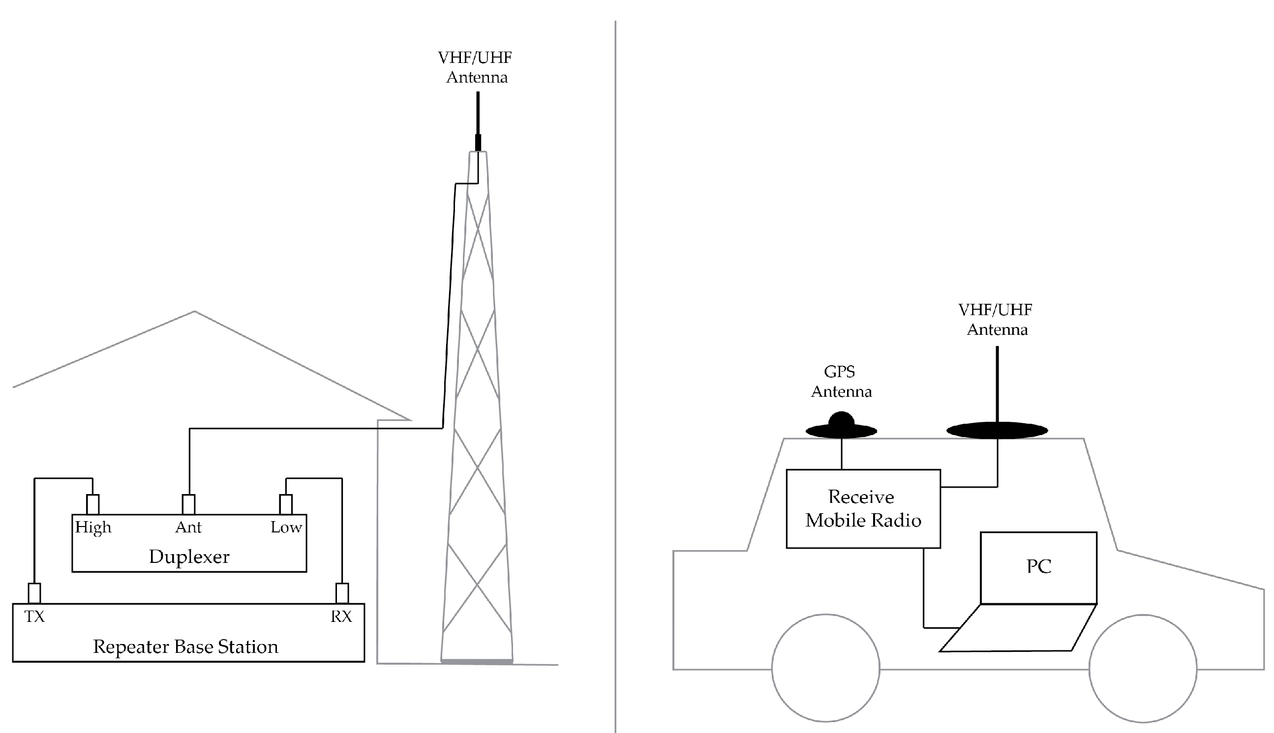
Figure 2 shows the set-up of the measuring system. The measurements on the measuring route were made first for the VHF system. Then, we changed the type of base-station and antenna and repeated the measurements for the UHF system. In this way, we avoided the unnecessary introduction of attenuations and interferences into the measurement system.

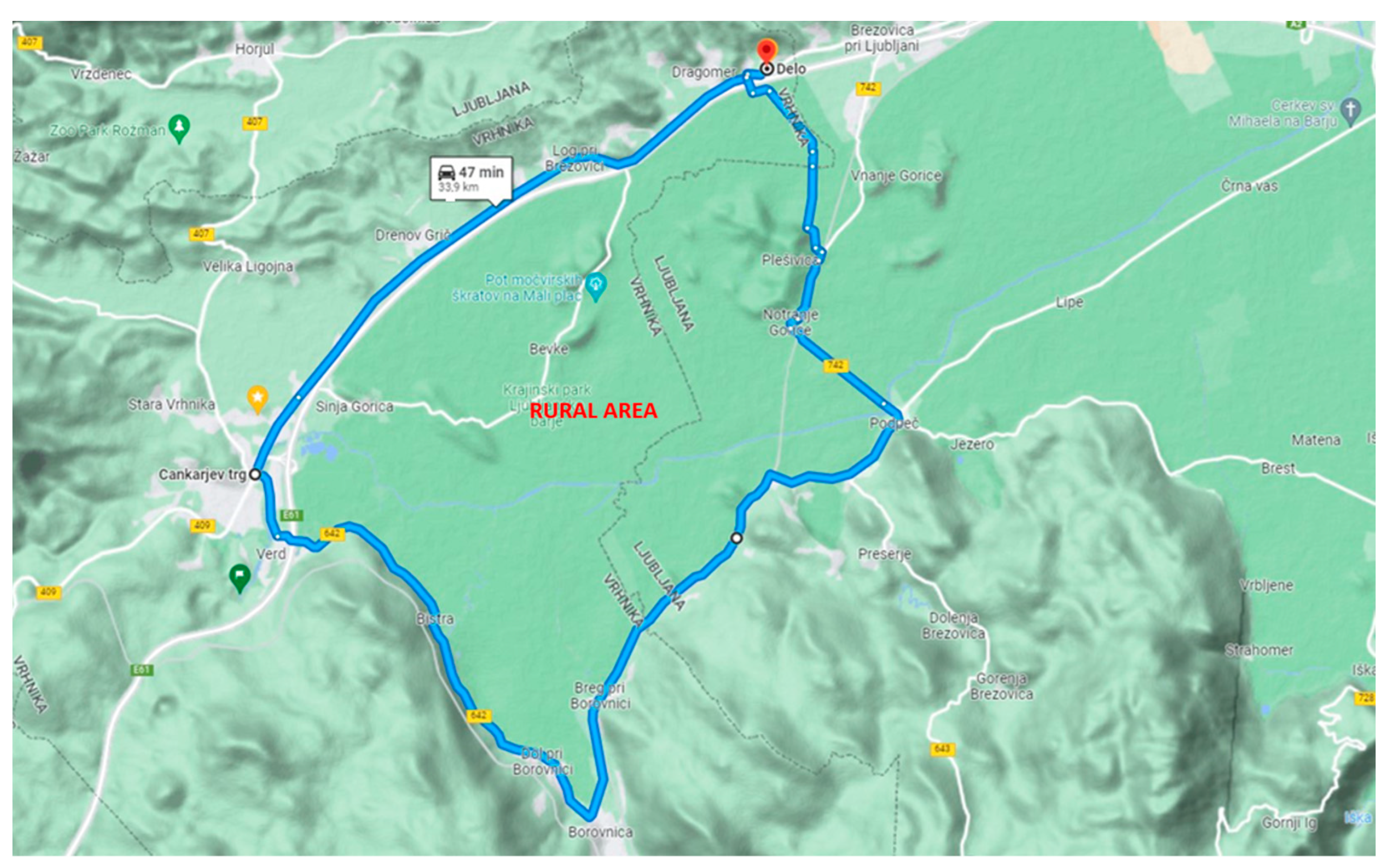
2.3. Test Route

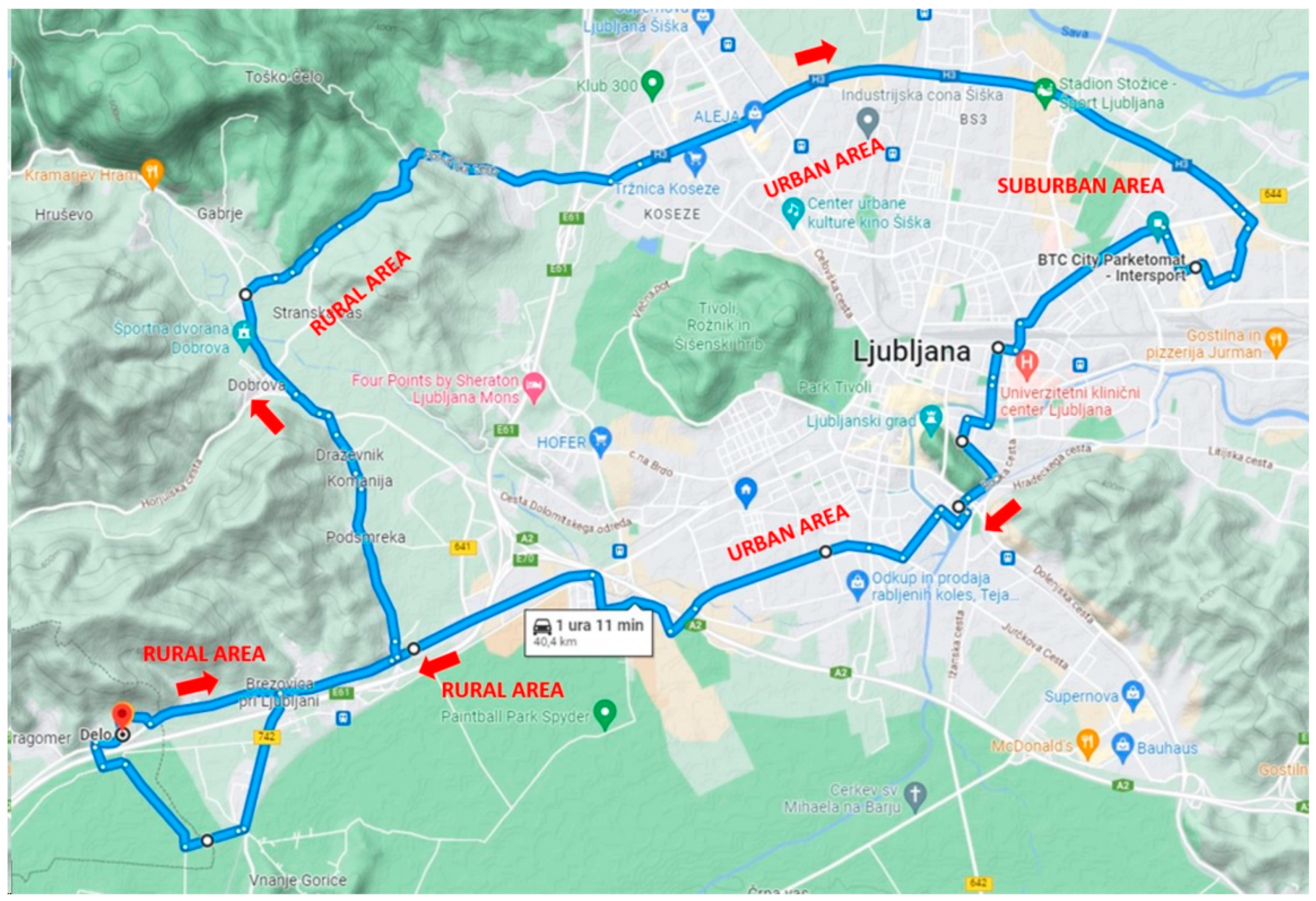
The field measurements were made on a 40 km long route around Ljubljana and its surroundings. The purpose of the selected test route was to include various terrains (flat and hilly terrain, different densities of buildings and vegetation) that can influence the propagation of radio waves and their calculations. The suitability of each model for calculating the attenuation in specific situations was evaluated based on the results of field measurements. The selected test route included rural, suburban, and urban areas. Approximately one-third of the route was within the line of sight of the transmitting antenna, while the rest was partially or completely obstructed by one or more hills, which were predominantly forested and represented obstacles between the transmitting and receiving antennas. The selected test route for both the VHF and UHF bands was the same and is shown in Figure 3.

3. Results

For computer calculations and field measurements with subsequent analyses, several computer programs and dedicated items of radio equipment were used. All the computer calculations were performed using TAP 7.5 software. The TAP Mapper 7.5 program was used for visualization and analysis of the calculated coverage as well as for comparing the calculated and on-site measured data and their visualization.

The calculated coverage areas made with the TAP Mapper 7.5 are color-coded to represent different levels of field strength. Each data point from the field measurements is represented by a small dot, which is colored according to the measured signal level.

Selected color coding for corresponding field strengths:

• Better than −80 dBm;
• −80 to −100 dBm;
• −100 to −110 dBm;
• −110 to −115 dBm;
• Worse than −115 dBm.

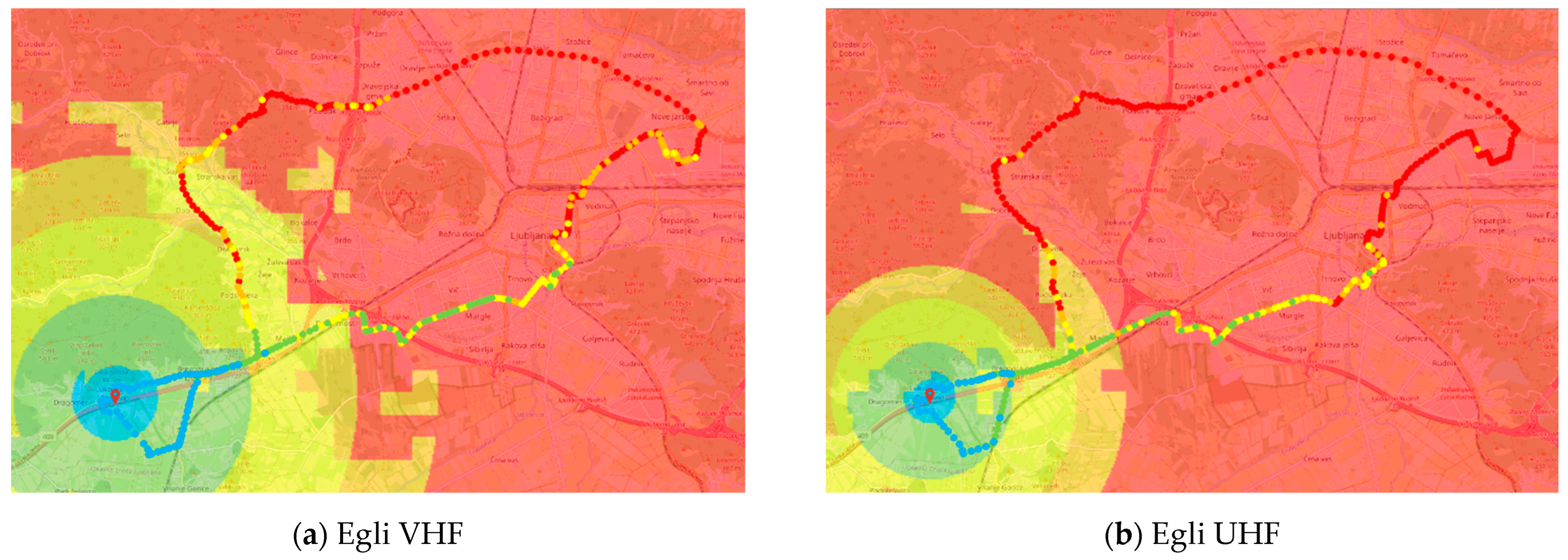
Figure 4 shows the predictions of the radio-signal level calculated using the Egli model. Additionally, the levels of the measured signal obtained from field measurements on the selected test route are shown for comparison. In the UHF band, there is a noticeable correction for higher frequencies, indicating that the attenuation along the path is more significant than in the VHF band.

It is clear from the figure that the model does not consider the actual terrain, as the field strength is primarily dependent on the distance to the transmitter and hardly affected by surrounding obstacles, such as hills, particularly north of the repeater base-station.

Figure 5 shows the coverage prediction with the radio signal according to the Okumura model. In the VHF-band calculation, the “Quasi-Open” correction was applied. This gave the best match with the field measurements on the selected test route among all terrain adjustments. Surprisingly, in the UHF band, the “Open” correction provided the best match with the field measurements.

Figure 6 shows the coverage prediction for the selected test route according to the Hata–Davidson model. Like the Egli model, the Hata–Davidson model also poorly considers large natural obstacles such as the hills north of the base-station location. However, unlike the Okumura model, the Hata–Davidson model provided the most accurate prediction in the VHF band with the “Urban Medium” correction and in the UHF band with the “Suburban” correction.

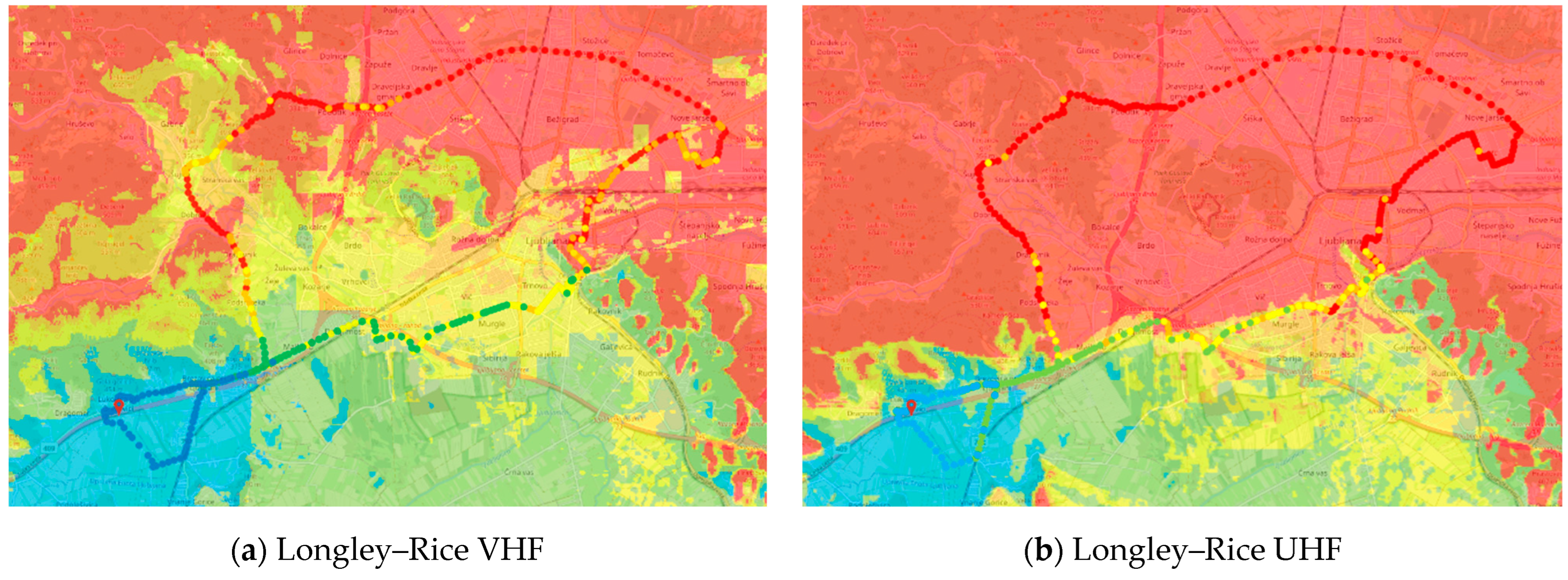
Figure 7 shows the coverage prediction using the Longley–Rice model. Additionally, the field strengths obtained from the field measurements on the selected test route are also present in the image. It is evident that there is excellent accuracy in fitting and higher resolution in the predictions relating to the natural obstacles especially in the VHF band. In the UHF band, there is a slight overestimation of attenuation especially in shaded areas without line-of-sight visibility.

4. Discussion

To compare the measured values with the calculated values, we used the procedures described in more detail in [11]. The deviation of the calculations compared to the field measurements for different models and frequency bands (VHF and UHF) is graphically represented in Figure 8, Figure 9, Figure 10 and Figure 11.

During the plotting of the graphs, 10 percent of the samples with the highest deviation between the calculated and measured values were always excluded from the analysis. This was to eliminate the most significant errors in the field measurements and the largest discrepancies in the calculations, which were usually observed in the immediate vicinity of the transmitter, where the field is very high and is rapidly changing. Additionally, it is essential to consider that various factors influence the results of field measurements, such as the proximity of larger vehicles, reflections, interference, vegetation, etc. This means that the results of the field measurements are not very accurate, as all these factors contribute to the variability of the received signal strength at each individual micro-location.

The average deviation of the Egli model’s attenuation in the VHF band is as high as 14 dB. Despite not considering the actual terrain, on average, the model introduces 11 dB higher attenuation than the actual values.

Similarly, in the UHF band, the Egli model introduces higher attenuation. The average deviation on the test route in the UHF band is as high as 16.6 dB more than the measured values. The average deviation reaches almost 18 dB when comparing the predicted values with the measured field strengths across the entire test route.

Based on the above findings, the Egli model has limitations and is practically unusable in an environment like the selected test route. A partial improvement in the attenuation prediction can be achieved by inputting the effective height of the transmitting or receiving antenna. This is probably one of the reasons why the predictions using the Egli model are much worse than the actual values in this case. The location of the base-station was on a small hill in the vicinity of Ljubljana. However, in the calculation, the relative height of the antenna above the ground was given, and the effective height of the antenna can be 20 to 30 m higher than the relative height entered for the transmitting antenna.

Due to its simplicity, the Egli model is one of the fastest for attenuation calculations. However, it should only be used in circumstances that match its assumptions, which do not include significant obstacles or more rugged terrain, as covered by our test route. The Egli model is limited to geographic areas with flat terrain and might only useful for the plains of northeastern Slovenia.

From Figure 9, it is evident that the Okumura model provides very accurate predictions of the signal propagation in both the VHF and UHF bands. In the VHF band with the “Quasi-Open” correction, the predicted signal strength deviates on average by only 4.3 dB. In the UHF band with the “Open” correction, the deviation is 5.3 dB, which is the smallest deviation in the UHF band.

The Okumura model indeed considers all the diversities of the selected test route very well, but some comments are necessary. The choice of the correction that yielded the best results is not entirely logical. The selected test route included both rural and urban areas, with the urban area covering a significant part of the analyzed area. However, the corrections “Quasi-Open” and “Open”, which are intended for predominantly or completely open rural areas, provided the most accurate predictions. Given the selected test route, a more logical choice would be the “Suburban” correction. It should be noted that the “Suburban” correction for the VHF band, on average, calculated an attenuation that was almost 10 dB too high. The deviation was even higher in the UHF band. This indicates an overestimation of the attenuation by the Okumura model, as for predominantly rural areas, there are insufficient corrections to further adjust the model’s attenuation.

The Okumura model can be very accurate in certain cases, as observed in our test route. However, it is crucial to conduct some test measurements to determine the appropriate correction for the specific terrain type. Relying solely on the basic correction definitions is not sufficient. In cases where conducting test-coverage measurements is not feasible or the coverage area is predominantly rural, the Okumura model is not recommended.

From Figure 10, we see that the correct Gaussian distribution of the attenuation deviation is calculated by the Hata–Davidson model in the VHF band. However, the model’s predictions are still inaccurate with an average deviation of around 7 dB. In the UHF band, the deviation is slightly higher, averaging almost 8 dB.

The Hata–Davidson model shows improvements in determining correction values for different types of terrain compared to the Okumura model. However, the Hata–Davidson model exhibits larger deficiencies in rugged, hilly terrain, which were not detectable in the Okumura model. Based on the comparison of field measurements with calculations using the Hata–Davidson model, we can conclude that the model does not have critical shortcomings, but it is superficial. This means that it can be satisfactory in specific cases, but it is almost useless in cases with greater roughness and more uneven terrain, where the effective height of the transmitting antenna is even negative.

In the VHF band, we can observe a good match with the Longley–Rice model, having the smallest deviation among all the analyzed models, averaging only 4.1 dB. However, the situation is different in the UHF band, where the model introduces more attenuation on the transmission path than we obtain from the actual field measurements. On average, the model’s attenuation in the UHF band exceeds the field measurements by 8 dB with an overall average deviation of 10 dB. The average errors between the predictions compared to field measurements are summarized in the

Table 1. Average error between the predictions and field measurements at the primary test route.

	Average Error between Predictions and Field Measurements
Model	VHF Band	UHF Band
Egli	+14.0 dB	+17.8 dB
Okumura	+4.3 dB	+5.2 dB
Hata–Davidson	+7.3 dB	+8.0 dB
Longley–Rice	+4.1 dB	+10.2 dB

.

Based on an analysis of the measured data, the Longley–Rice model was the most accurate for predicting the propagation of electromagnetic waves in the VHF band. However, it does face some challenges in the UHF band, where it introduces excessive attenuation, especially in shadowed areas where there is no line of sight between the transmitting and receiving antennas, which constitute a part of the selected test route. One advantage of the Longley–Rice model is that it does not require manual adjustments of the corrections based on the type of terrain, since it utilizes topographical data from digital maps. This feature greatly simplifies the work for network planners, especially in cases where prior test field measurements are not feasible or the coverage area is extensive and geographically and urbanistically diverse.

Final Analysis and Additional Test Route

The selected test route provided valuable insights into the response of each model for coverage calculations in different scenarios encountered in radio-network planning. However, during the field measurements, some possible shortcomings of the primary test route and the equipment were identified.

A crucial point is related to the sensitivity of the Motorola DM4601e radio receiver, which was −123 dBm, with a noise floor threshold of −127 dBm. In certain cases, especially in the UHF band, the models predicted signal levels as low as −150 dBm, which the selected radio receiver could not measure. It simply registered the noise floor as the relevant usable signal level. Another issue, primarily observed in the VHF band, was that the receiver only recorded the Received Signal Strength Indicator (RSSI) on the selected channel. In Ljubljana BTC City (large shopping area), it happened that the base-station did not activate because the signal level was below the noise-floor threshold. However, due to various interferences on the measured frequency channel or strong signals in the adjacent frequency channels, the station detected and recorded an RSSI level better than −115 dBm. Such issues were not present in the suburban and rural areas. Considering these observations, we had doubts about the accuracy of the measurements below −115 dBm, especially in the UHF band and urban areas. Nevertheless, these measurements constituted a portion of the data within the selected test route.

To address the doubts about measurement accuracy, a secondary test route was established. It was more open, running through the outskirts of Ljubljana. A map of the secondary test route is shown in Figure 12. The secondary test route was essential to confirm or refute certain hypotheses from the primary test route with greater reliability. Additional measurements were particularly useful in the UHF band, where more discrepancies between the measurements and calculations were observed on the primary test route.

It is important to emphasize that the secondary test route was selected in a much more open area between the transmitter and receiver. There were only minor natural obstacles compared to the primary test route. The measured signal levels in the secondary test route were always better than −115 dBm, which excluded the shortcomings of the radio equipment used for measuring.

In the UHF band of the secondary test route, the Egli model introduced even greater attenuation, exceeding 20 dB in this case. The Okumura model, despite using the correction for an open area, still calculated an average attenuation that was 6 dB too high. The Hata–Davidson model with “Quasi-Open” correction and Longley–Rice model performed the best, but they still had some deviations. For instance, the Hata–Davidson model considered very generalized smoothing and neglected shadowed areas, and the Longley–Rice model slightly overestimated the average attenuation in the shadowed areas. The results of the measurements on the secondary route are collected in

Table 2. Average error between the predictions and field measurements (UHF only) on the secondary test route.

	Average Error between Predictions and Field Measurements
Model	UHF Band
Egli	+23.9 dB
Okumura	+9.1 dB
Hata–Davidson	+7.9 dB
Longley–Rice	+7.6 dB

.

The larger discrepancies in the UHF band could potentially be attributed to a thin layer of frozen wet snow present during the field measurements. However, according to [12], there is no significant difference between the effects of ice crust, ice drops or melted snow on the attenuation for this frequency band. Additionally, the relative dielectric constant or relative permittivity of dry snow is independent of the frequency from 1 MHz to at least 10 GHz [12]. Some sources even predict higher ground attenuation in the winter months [13,14]. Therefore, the larger discrepancies cannot be solely attributed to the weather conditions, although spring foliage would likely result in slightly higher attenuation than was measured in mid-December. This would lead to better alignment between the field measurements and the calculations.

The quality of the predictions for radio-network planning can be greatly improved by machine-learning methods [15]. In particular, supervised learning can model hidden nonlinear relationships and can therefore be used for path-loss prediction. To achieve a good agreement with the measured data and the prediction model, our collected data can also be used for training in the future. The data collected in this work can be accessed here [16,17].

5. Conclusions

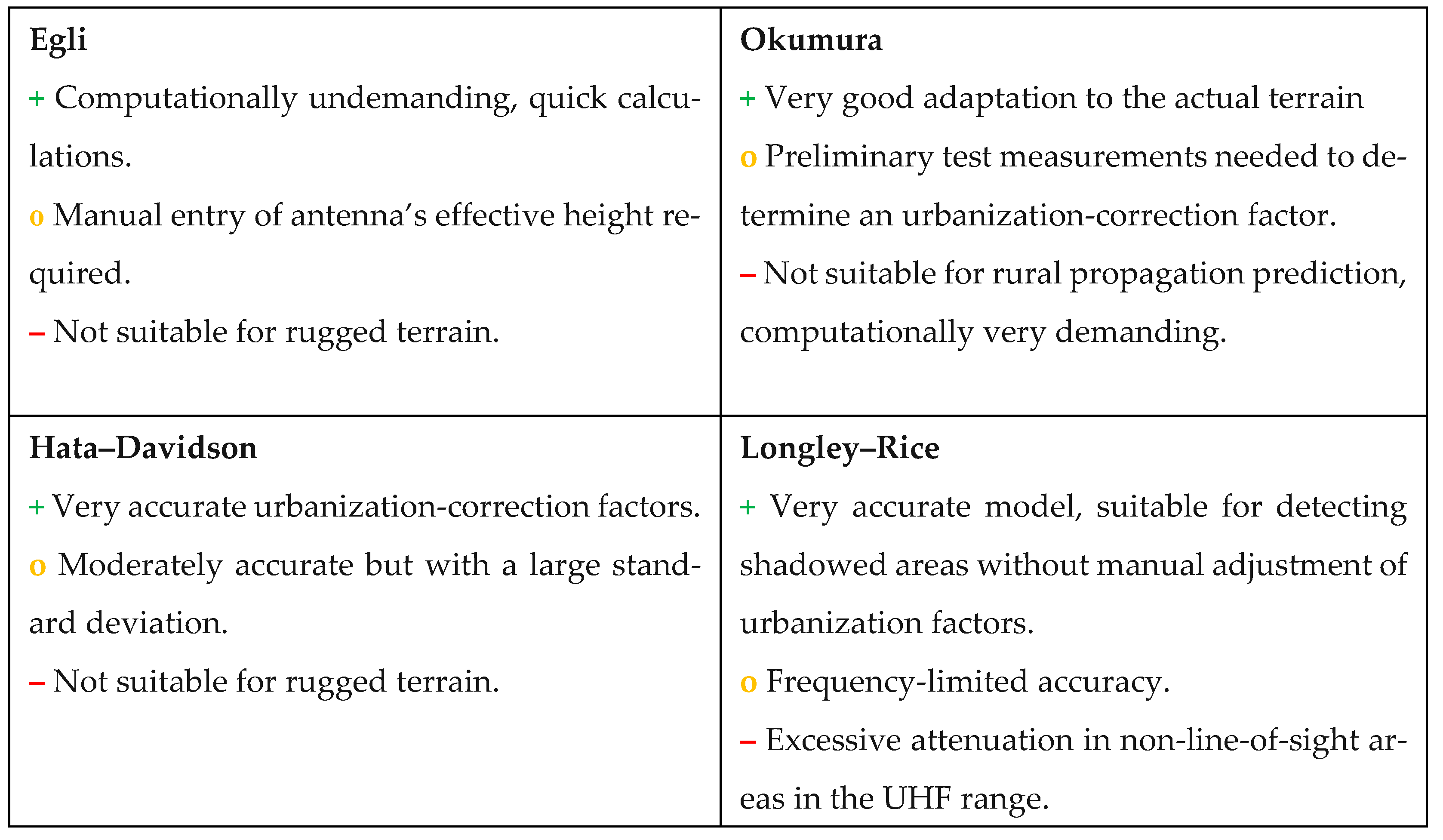
With the comparison of the calculations from different models using various settings and adjustments in the primary and secondary test routes, it was confirmed that we must exercise great caution when using an individual model or its specific adjustments. Among the analyzed models for path-loss calculations, there is no model that can be deemed the most accurate in all cases. Each model has its own advantages and limitations, as summarized in Figure 13.

The basic Egli model initially appears to be very inaccurate, but this can be improved by inputting effective antenna heights. Moreover, Egli’s calculations are the least computationally demanding, making it the fastest model. In the UHF band, the Egli model can be compared to the Okumura and Hata–Davidson models using a correction for the urban area. However, in both the primary and secondary test routes, the predictions for path losses were overestimated.

Although the Okumura and Hata–Davidson models share a similar theoretical foundation, they do not show many parallels in practice. The Okumura model accurately accounts for the path loss in the shadowed areas but tends to introduce an overall higher path loss in the transmission path. It is ideal for nearly open and completely open areas. The use of terrain corrections requires extensive experience, caution, and continuous validation through individual field measurements if possible. In terms of terrain-urbanization corrections, the Hata–Davidson model is undoubtedly ahead of the Okumura, as its characterizations proved to be more suitable and predictable. However, Hata–Davidson faces significant challenges in shadowed areas where it does not properly consider the path loss caused by natural obstacles. Another difference between the models lies in the complexity of their calculations. For a grid coverage calculation of 20 × 20 km², the Hata–Davidson model required approximately 45 min, while the same calculation with the Okumura model took more than 12 h. This can be a substantial obstacle when using the model frequently.

The Longley–Rice model proved to be the most flexible and generally applicable model, allowing adjustments and demonstrating high accuracy. This is valid, especially in the VHF band, and with some limitations also in the UHF band. The limitations are mainly evident as excessive path losses in shadowed areas without a line of sight between the transmitting and receiving antennas. Nevertheless, the Longley–Rice model provides predictions with great accuracy and resolution for smaller shadowed gaps and open areas. This makes it ideal for identifying blackspots and other geographical peculiarities where all the other models exhibited excessive generalization and smoothing.

The conclusion is that even very complex models that include a whole range of corrections (e.g., due to the type of terrain, vegetation, buildings, curvature of the earth, etc.) do not provide substantially better results than simpler models.