Article

Comparative Study of Sentinel-1-Focused and Simulated SAR Images Using LiDAR Point Cloud Modeling for Coastal Areas

1
School of Physics and Electronic Information, Yanan University, Yan’an 716000, China
2
Key Laboratory for Information Science of Electromagnetic Waves (MoE), Fudan University, Shanghai 200433, China
3
Institute for Radio Frequency Technology and Software, Beijing Institute of Technology, Beijing 100081, China
*
Author to whom correspondence should be addressed.
Electronics 2023, 12(20), 4312; https://doi.org/10.3390/electronics12204312
Submission received: 4 September 2023 / Revised: 8 October 2023 / Accepted: 16 October 2023 / Published: 18 October 2023
(This article belongs to the Special Issue Microwave Imaging Technology)

Abstract

:
Aiming at SAR imaging for large coastal scenes, a comprehensive comparative study is performed based on Sentinel-1 raw data, SAR imaging simulation, and Google Maps. A parallel Range-Doppler (RD) algorithm is developed and applied to focus Sentinel-1 raw data for large coastal scenes, and the focused SAR image is compared with the multi-look-processed SAR image using SNAP 9.0.0 software, as well as the corresponding areas of Google Maps. A scheme is proposed to convert the LiDAR point cloud data of the coast into a 3D coastal area digital elevation model (DEM), and a tailored 3D model suitable for RaySAR simulator is obtained after statistical outlier removal (SOR) denoising and down-sampling processing. Comparison results show good agreements, which verify the effectiveness of the parallel RD algorithm as well as the backward ray-tracing-based RaySAR simulator, which serves as a powerful SAR imaging tool due to its high efficiency and flexibility. The cosine similarity between the RaySAR-simulated SAR image and Google Maps achieves 0.93, while cosine similarity reaches 0.85 between Sentinel-1 SAR-focused images with our parallel RD algorithm and multi-look SAR image processed using SNAP software. This article can provide valuable assistance for SAR system performance evaluation, SAR imaging algorithm improvement, and remote sensing applications.

1. Introduction

Synthetic Aperture Radar (SAR) imaging techniques have been increasingly extensively applied in various fields [1,2,3,4,5], such as military reconnaissance, ocean remote sensing, meteorological observation, and various other domains, due to its day–night and all-weather monitoring capability [6,7,8,9] Among these, earth observation is one of the most significant applications of SAR [10,11], enabling mapping, geological exploration, environmental monitoring, and resource survey [12]. All of these applications leverage SAR data [13] and rely strongly on advanced imaging algorithms for efficient and accurate imaging. SAR was first proposed and utilized in the late 1950s on RB-47A and RB-57D strategic reconnaissance aircrafts [14]. In June 1978, SEASAT successfully launched and marked the beginning of spaceborne SAR technology. In order to process SEASAT SAR data, the Jet Propulsion Laboratory (JPL) proposed a new digital signal processing algorithm that could make an approximate separation of the two directions using the significant difference between range and azimuth time. This algorithm, called the Range-Doppler (RD) algorithm [15,16,17], performs range cell migration correction (RCMC) in the Range-Doppler domain [18,19,20]. In 1984, Jin and Wu [21] in JPL discovered the phase coupling between range and azimuth and then improved the RD algorithm by implementing second range compression (SRC), making the algorithm capable of dealing with SAR medium squint angle. Since then, developments in RCMC and secondary range compression have allowed the RD algorithm to deal with SAR with high squint angle [22,23,24], and the RD algorithm has been widely used in SAR imaging due to its high efficiency and accuracy.
From two perspectives of imaging simulation and real SAR raw data processing, SAR has been studied in the past decades. The significance of SAR imaging simulation is to help professionals in military, scientific, and industrial fields understand and evaluate the performance, characteristics, and limitations of SAR technology. SAR imaging simulation enhances researchers’ understanding of SAR systems and is a basis for building real SAR systems. For SAR imaging simulation, researchers try to develop SAR simulators, including geometrical modeling, raw echo generation based on computational electromagnetics, as well as radar signal processing to obtain SAR images. For example, F. Xu, in 2006, proposed a comprehensive approach to simulate polarimetric SAR imaging for complex scenarios, which considers the scattering, attenuation, shadowing, and multiple scattering effects of volumetric and surface scatterers distributed in space [25]. In the same year, G. Margarit et al. proposed a SAR simulator, GRECOSAR [26], which is applied to complex targets and can provide PolSAR, PolISAR, and PolInSAR images. In addition, RaySAR [27,28] as a SAR imaging simulator was developed by S. Auer in his doctoral thesis [29] in 2011 at the Technical University of Munich in collaboration with the German Aerospace Center (DLR, Institute of Remote Sensing Technology). Due to its high efficiency and flexibility, RaySAR can generate very high-resolution SAR products based on backward ray tracing techniques [30,31,32]. In 2022, MetaSensing developed a simulator, KAISAR [33], based on GPU acceleration and ray tracing methods, which can efficiently generate SAR images for complex 3D scenes. Due to its extremely high efficiency in evaluating electromagnetic scattering, the ray tracing method can efficiently calculate radar echoes for large-scene SAR imaging simulation. The classical ray tracing methods are forward ray tracing, backward ray tracing, and hybrid ray tracing. On this basis, many researchers have improved the ray tracing method. Xu and Jin proposed a Bidirectional Analytic Ray Tracing (BART) method [34] to calculate the composite RCS of a 3D electrically large complex target above a random rough surface. In [35], Dong and Guo proposed an accelerated ray-tracing algorithm, which is accelerated using the neighbor search technique, with a new 0–1 transformation rule and arrangement of octree nodes. This algorithm improved the computational efficiency of the composite scattering of 3D ship targets on random sea surfaces.
As a basis for SAR imaging simulation, 3D modeling is an indispensable step in the SAR imaging system. There are many methods for modeling complex 3D scenes, such as through Computer-Aided Design (CAD) modeling, mathematical modeling, etc. From point clouds, 3D models of complex scenes can be efficiently built, among which Light Detection and Ranging (LiDAR) [36,37,38] can quickly obtain a large amount of point cloud data, which is more efficient than traditional measurement methods. This technique is of great importance for applications such as modeling large-scale scenes, quickly updating models, and so on. As a new model reconstruction technology in recent years, LiDAR point cloud modeling technology has been extended to various application fields and plays an important role in many fields, such as digital city, engineering planning, ancient architectural protection, and so on. In [39], a new method for extracting buildings from LiDAR data was proposed by Ahmed F. Elaksher et al., and this method uses the geometric properties of urban buildings to reconstruct building wireframes from LiDAR data. In [40], a novel CNN-based method was developed, which can effectively address the challenge of extracting the Digital Elevation Model (DEM) in heavily forested regions. By employing the concept of image super resolution, this approach achieves satisfactory results without requiring the use of ground control points. Recently, a set of effective, fast 3D modeling methods was presented, which can realize the modeling of 3D point clouds of different sites and has a good modeling effect [41].
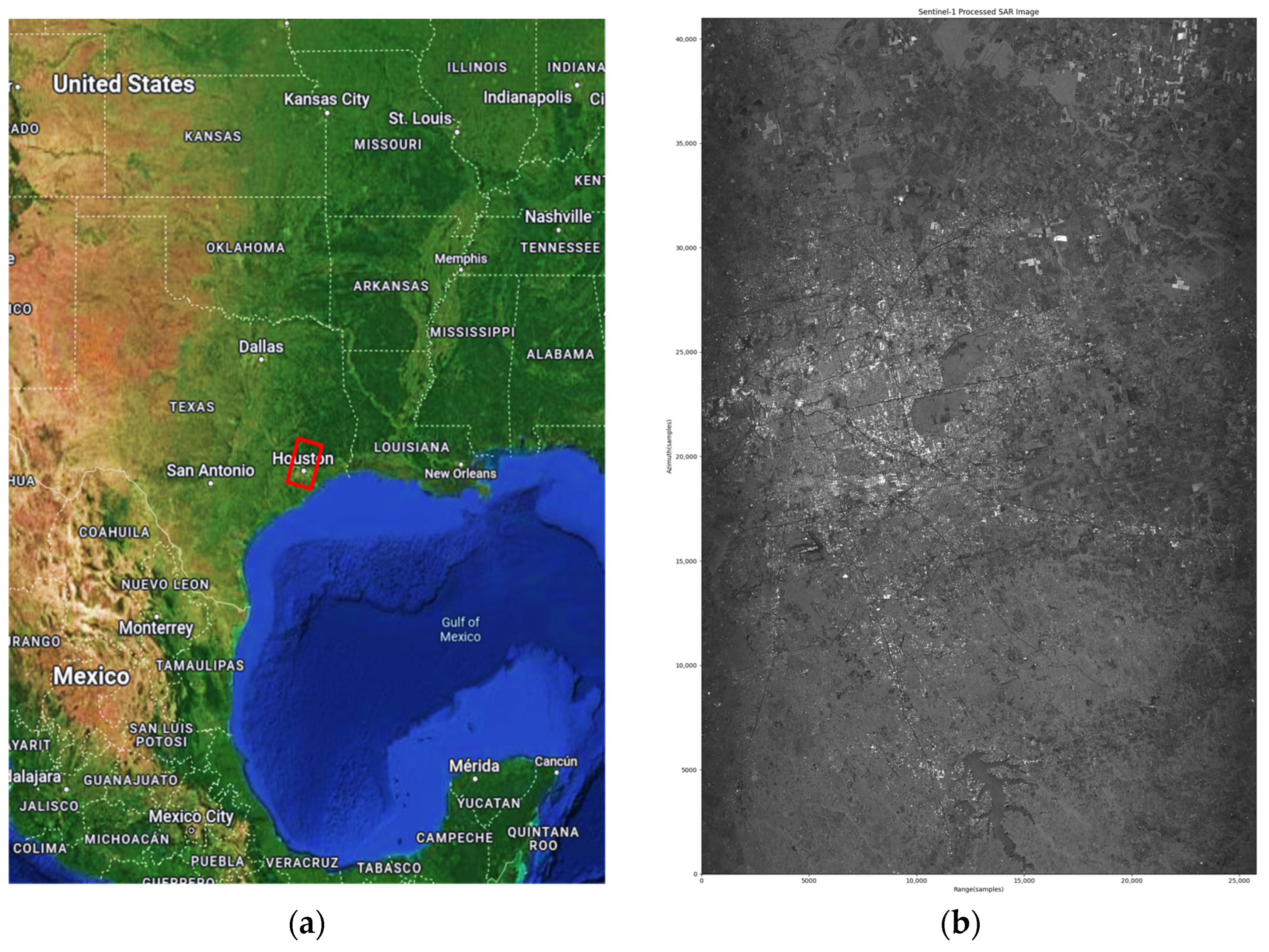
With the continuous launch of SAR missions, ERS-1, Radarsat-1, TerraSAR, Sentinel-1, GF-3, etc., can continuously provide massive SAR products for researchers. Typically, the Sentinel-1 consists of a constellation of two polar-orbiting satellites, Sentinel-1A and Sentinel-1B [42], operating day and night to perform C-band SAR imaging. Level-0, Level-1, and Level-2 data products are provided for user use. Most researchers are using Level-1 and Level-2 products for their research, such as target recognition and feature extraction from SAR images. However, for processing Level-0 raw data, there are few publicly available commercial software for technical support. M. Kirkove developed a SAR processor for Terrain Observation by Progressive Scans (TOPS) based on the Omega-K Algorithm [43]. The processor combined preprocessing by frequency unfolding and post-processing by time unfolding. In addition, K. Kim et al., in 2021, processed and sorted the Sentinel-1 Level-0 raw data via swath, and they generated a SAR-focused image of Seoul City [44].
Aiming at SAR imaging for large coastal scenes, this paper is devoted to a comprehensive comparative study on spaceborne SAR imaging of coastal areas by virtue of Sentinel-1 raw data, SAR imaging simulation, and Google Maps. In comparison with free and publicly available DEM data with accuracies typically 30 m and 90 m, the accuracy of LiDAR point cloud data can reach the sub-meter level. Hence, for large coastal scene modeling problems encountered in SAR imaging simulation, a tailored 3D DEM model is to be developed in this paper, which is converted from the LiDAR point cloud data of the coastal areas by performing statistical outlier removal (SOR) denoising and down-sampling processing.
This paper is organized as follows: Section 2 introduces the Range-Doppler algorithm and its parallel implementation. In Section 3, the modeling of coastal areas and SAR imaging simulations are presented. In Section 4 and Section 5, results and discussion are presented, and a comprehensive comparison is made among the simulated SAR image of selected 3D coastal areas, the focused SAR image of Sentinel-1 data, the multi-look-processed SAR image using SNAP software, as well as the corresponding areas of Google Maps. Section 6 concludes this paper.

2. Range-Doppler Algorithm and Its Parallel Implementation

The Range-Doppler (RD) algorithm operates approximately in the range direction and the azimuth direction, and the processing procedure could be carried out in two one-dimensional operations due to the large difference in time scales of the range and azimuth echo [45]. In the RD algorithm, the radar echo data are processed via range pulse compression, range cell migration correction (RCMC), and azimuth pulse compression, respectively. After the aforementioned procedures, the focused SAR image is obtained finally.
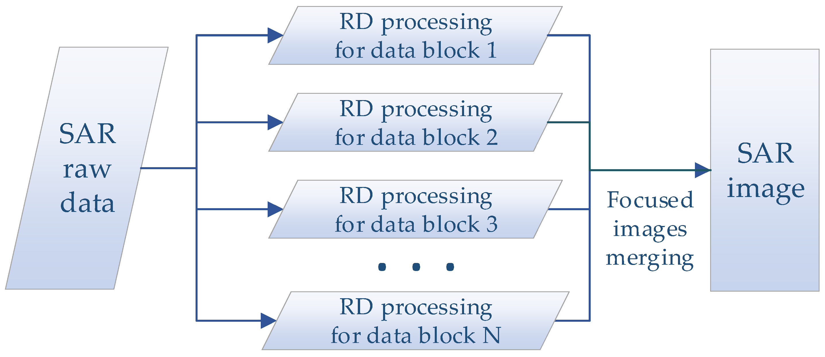
Although the conventional RD algorithm is very efficient in processing SAR raw data due to the use of fast Fourier transform (FFT), it also encounters challenges when dealing with large-scene SAR data. Because SAR raw data is inherently suitable for parallel processing, a scheme for parallel processing SAR echoes is presented in this paper, in which the SAR raw data are divided into N blocks in the azimuth direction and can thus be processed parallelly.

2.1. SAR Echo Model

The transmitted pulse of the linear frequency modulation signal S p u l ( τ ) can be expressed as follows:
S p u l ( τ ) = ω r ( τ ) cos ( 2 π f 0 τ + π K r τ 2 )
where K r is the range compression chirp rate, f 0 is the center frequency [46,47], and τ is the range direction time. ω r ( τ ) is a rectangular signal or window function to define a finite signal S p u l .
ω r ( τ ) = { 1 , | τ T | 1 0 , e l s e w i s e
In Equation (2), T is the pulse duration. The reflected energy of the radar at any time of illumination S r is a convolution of the pulse waveform at that time and the scattering coefficient g r of the scene in the illuminated area.
S r ( τ ) = g r ( τ ) S p u l ( τ )
For a point target at range R a from the radar with a backscattering coefficient A 0 , g r can be expressed as follows:
g r ( τ ) = A 0 δ ( τ 2 R a / c )
where c is the speed of light. Since R a varies with the azimuth time η , which can be denoted as R ( η ) , η c is the azimuth time when the sensor is closest to the target. The two-dimensional received signal S r ( τ , η ) in the time domain of the point targets can be expressed as follows:
S r ( τ , η ) = A 0 ω r ( τ 2 R ( η ) / c ) ω a ( η η c ) × cos [ 2 π f 0 ( τ 2 R ( η ) / c ) + π K r ( τ 2 R ( η ) / c ) 2 ]
where ω a is a rectangular signal or window function, similar to ω r .

2.2. RD Algorithm

We perform range pulse compression on the raw echo signal. The received signal s r contains the radar carrier frequency, cos ( 2 π f 0 τ ) . Before sampling, it needs to be down-converted using the method of orthogonal demodulation. The Fourier transform in the range direction is applied to the demodulated signal, and the frequency spectrum in the range direction can be obtained. The range pulse compression is completed by multiplying it with a matched filter in the frequency domain and then performing an inverse Fourier transform [48]. The expression of the range-compressed signal S r c ( τ , η ) in the time domain can thus be expressed by the following:
s r c ( τ , η ) = A 0 sinc [ B r ( τ 2 R ( η ) c ) ] ω a ( η η c ) exp { j 4 π f 0 R ( η ) c }
where
p r [ τ 2 R ( η ) / c ] = sinc [ B r ( τ 2 R ( η ) / c ) ]
A greater slant angle results in an increased range and azimuth coupling when the slant angle is not zero. A second range compression (SRC) procedure is required to correct the defocus caused by the coupling for more precise imaging. To solve this problem, after range compression using a matched filter with a chirp rate of K r , a filter with a chirp rate of K s r c should be applied as a secondary filter for compression. This filter H s r c can be expressed as follows:
H s r c ( f τ ) = exp { j π f τ 2 K s r c ( R 0 , f η ) }
Here, R 0 is the range when the target is closest to the radar. f τ is the range frequency, and f η is the azimuth frequency.
Next, we perform RCMC. The same target is compressed to different positions in different azimuth directions, that is range migration. In the time domain, multiple targets may be present in different azimuth cells at the same range cell, so it is difficult to correct each target separately. After the Fourier transform of the range-compressed signal in azimuth direction, the targets in the same range cell can be corrected uniformly in the Range-Doppler domain. The RCMC formula is given by the following:
S r c m c ( m , n ) = S r c ( m , n + 2 R × F s c ) = S r c ( m , n + n + n )
where m and n are the number of sampling sequences in the azimuth and range directions. F s is the sampling frequency in the range direction. R is the range migration. P R F is the pulse repetition frequency. n is the integer part of 2 R × F s / c , and n is the fractional part. Hence, the processing of range migration is completed. Applying sinc interpolation, the range migration corrected signal S r c m c ( τ , f η ) is as follows:
S r c m c ( τ , f η ) = A 0 p r ( τ 2 R 0 c ) W a ( f η f η c ) × exp { j 4 π f 0 R 0 c } exp { j π f η 2 K a }
where K a is the azimuth chirp rate. Subsequently, we perform azimuth pulse compression. The azimuth-matched filter H a z ( f η ) is the complex conjugate of the second exponential term, which is expressed as follows:
H a z ( f η ) = exp { j π f η 2 K a }
The RCMC-processed signal S r c m c ( τ , f η ) is multiplied by the frequency domain-matched filter H a z ( f η ) . After the inverse Fourier transform, the azimuth compression is completed as follows:
s a c ( τ , η ) = I F F T η { S a z ( τ , f η ) } = A 0 p r ( τ 2 R 0 / c ) p a ( η ) × exp { j 4 π f 0 R 0 c } exp { j 2 π f η c η }
Here, p a is the amplitude of the azimuth impulse response, similar to p r , which is the sinc function. s a c ( τ , η ) is the 2D time-domain signal obtained after processing with the Range-Doppler algorithm.

2.3. Parallel Implementation for RD Algorithm

RD algorithm is used to process the raw echo signal of SAR, and the processing efficiency is excellent due to the use of FFT. However, for a large amount of SAR raw data, the conventional RD algorithm still takes a long time. In order to solve this problem, we analyzed the way the raw signal is collected and the data composition structure. In SAR system, the sensor collects the range direction signal in turn at each azimuth sampling point in a “stop-go-stop” manner. In short, the SAR raw echo signal is collected in a linear manner in the azimuth direction.
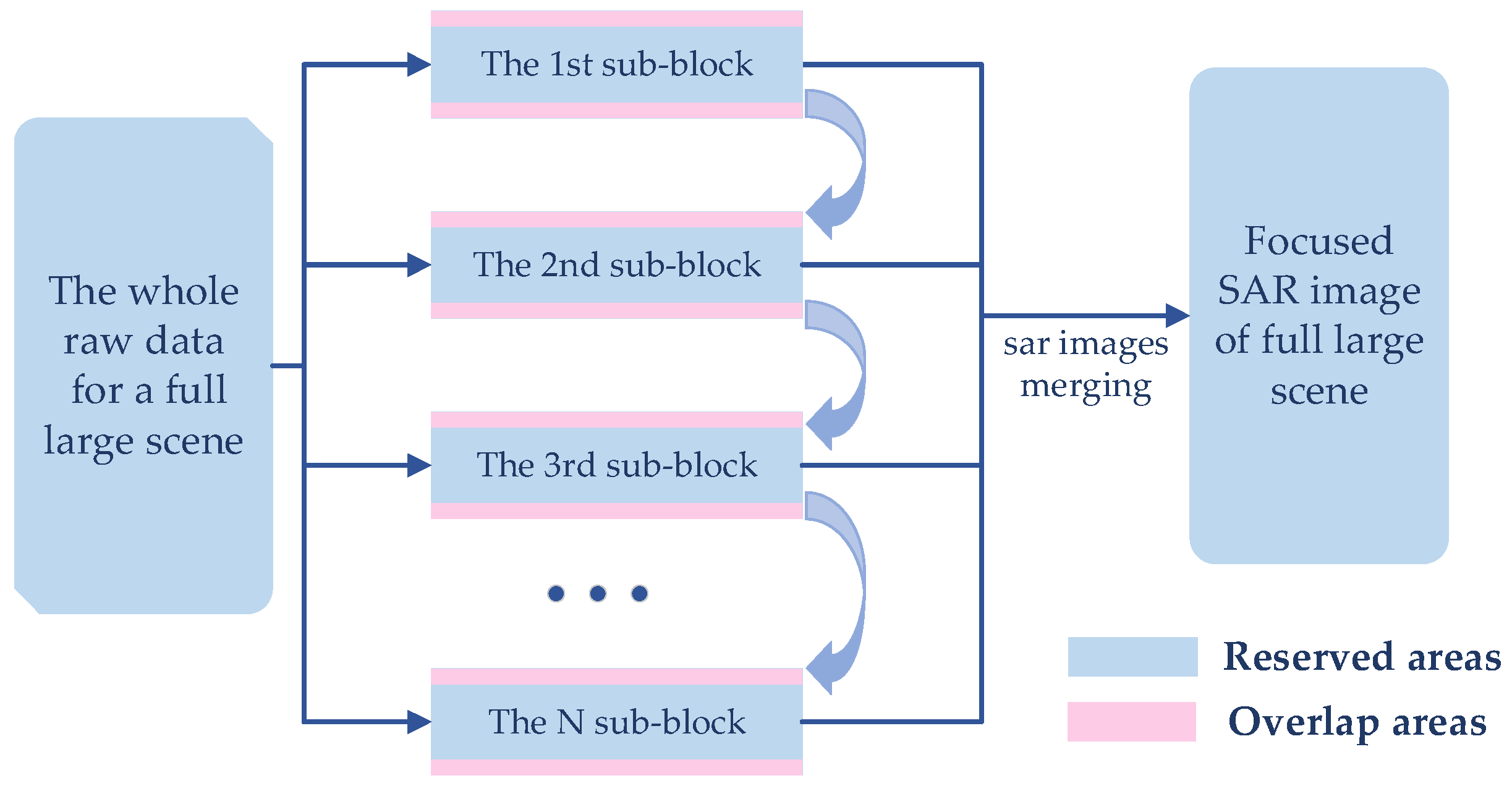
Using this feature, to further improve the processing efficiency, a parallel scheme for processing a large amount data using the RD algorithm. The flow chart of our parallel scheme is illustrated in 
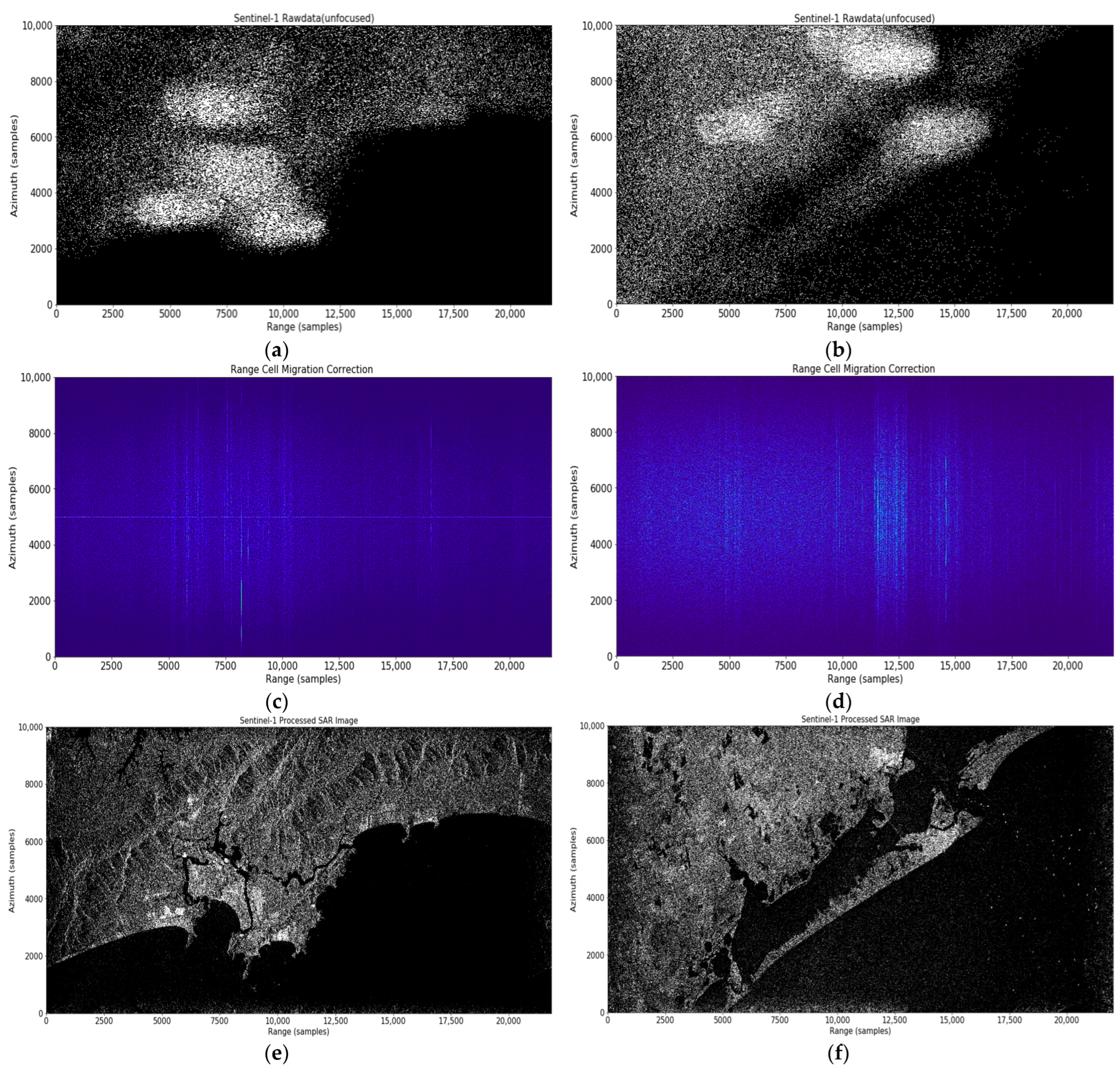
Figure 1. The raw echo signal is divided into N blocks according to the azimuth sampling points, and each divided data block is processed with the RD algorithm at the same time. Since the range sampling point of the raw echo signal is not changed, all the data blocks can be easily merged after SAR imaging processing. Our scheme allows a good combination of the characteristics of SAR systems with a parallel acceleration technique. For example, our parallel scheme is applied to SAR raw data with 8000 and 27,000 sampling points in the azimuth and range directions, respectively. The sampling points are divided into four equal data blocks along the azimuth direction. The results show that our parallel acceleration method takes only 34.1% in comparison with the serial processing time, resulting in a significant improvement in processing efficiency.

3. Coastal Areas Modeling and SAR Imaging Simulation

Coastal areas include land and sea surfaces, with buildings, hillsides, and roads on land as well as piers and bridges on water. It is difficult to model the real coastal areas because the structure of the coastal areas is complex. Light Detection and Ranging (LiDAR) point cloud data have the advantages of high resolution and sufficient available data, which are suitable for constructing complex 3D coastal area models. Therefore, in this paper, we process the Light Detection and Ranging (LiDAR) point cloud data by denoising and down-sampling, and then, we triangulate the LiDAR point cloud data to establish a 3D model of the coastal areas. Based on this model, we use the ray tracing method to realize the simulation of spaceborne SAR imaging. The block diagram of a comprehensive comparative study for coastal areas is illustrated in Figure 2.

3.1. LiDAR Point Cloud Data

In order to model the real coastal areas, we need a data source that carries coastal geographic information. The higher the accuracy of the data source, the more realistic the coastal areas model will be. LiDAR point cloud data meet our need for model accuracy. LiDAR is a remote sensing technique that utilizes laser light to measure the elevation of various objects such as buildings, ground surfaces, and forest areas. It employs ultraviolet, visible, or near-infrared sources to detect and analyze these objects. LiDAR determines the distance by measuring the time taken for the signal to travel from sensor to target and back to sensor, providing a measurement of objects on the ground.
This enables the creation of a precise and reliable 3D representation of Earth’s surface, facilitating the modeling of both natural and man-made features with high accuracy. The applications of LiDAR have a variety of fields, including agriculture, forest management, architecture, transportation and urban planning, surveying, geology, mining, heritage mapping, etc.
LiDAR point cloud is a technique that uses lidar to scan the surface of an object and convert the reflected laser beam into 3D coordinate points to form a data set [36,41]. An average LiDAR data product comprises a large amount of point cloud data, ranging from millions to billions of precise 3D points [37,38] denoted by their coordinates (X, Y, and Z). This data set also includes supplementary attributes like intensity, feature classification, and GPS time. These additional attributes are essential and supplemental information when creating a 3D model [40].

3.2. Approach to Model Realistic Coastal Areas

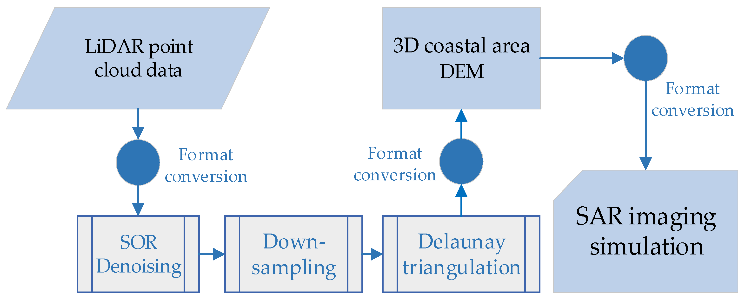
In order to model the real coastal areas, a scheme is proposed to convert the point cloud data of the coast into a 3D coastal area DEM. The point cloud data with higher accuracy are more beneficial for modeling realistic coastal areas. The resulting DEM mesh can be utilized as an input geometrical model for SAR imaging simulation. The approach is to perform SOR denoising and down-sampling of LiDAR point cloud data, followed by Delaunay triangulation to generate a 3D coastal area DEM, which is used as a target for SAR imaging simulation. The flow chart of our approach to modeling the 3D coastal areas is shown in Figure 3.
According to the modeling procedure, a geometric model of actual terrain can be obtained. Next, we will discuss the modeling approach in detail, taking a part of the city of Vallejo for example, which is located in the San Francisco Bay area. The public LiDAR point cloud data can be downloaded from the Open Topography official website.
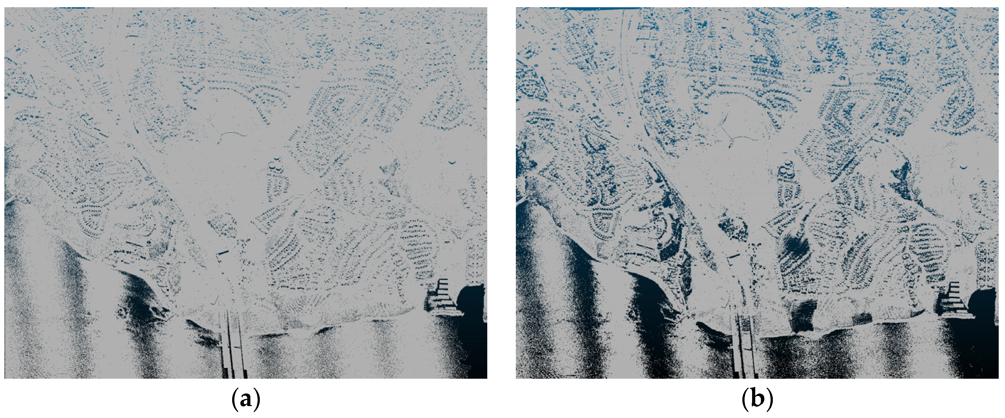
After downloading, the point cloud data are shown in Figure 4a. However, the presence of rain, fog, or dust can introduce noise to the original point cloud, such as outliers, which can heavily impact subsequent modeling tasks. To mitigate this problem, we perform a denoising step on the original point cloud using the SOR method. This method mainly carries out a statistical analysis on the neighborhood of each point. In terms of the distance distribution from a point to all adjacent points based on distance distribution, some points that do not conform to the requirements of outliers are filtered out.
The SOR procedure consists of two iterations. In the first iteration, the average distance of each point to its nearest N neighboring points is calculated, and the obtained results are in the form of Gaussian distribution. Then, the mean μ and standard deviation σ of these distances are calculated to determine the distance threshold Q , where Q = μ ± k σ . Here k is the multiplier of the standard deviation. For the second iteration, we classify points as inliers or outliers based on whether their average neighborhood distance falls below or above this determined threshold. As a result, Figure 4b shows the denoised point cloud data. By comparing Figure 4a and Figure 4b, it is observed that the distribution of all points is more regular after denoising the original point cloud data, in which some points higher or lower than the whole points are filtered out. If outliers are not removed, some spikes in Delaunay triangulation will appear on the surface of the generated model, leading to an inaccurate model.
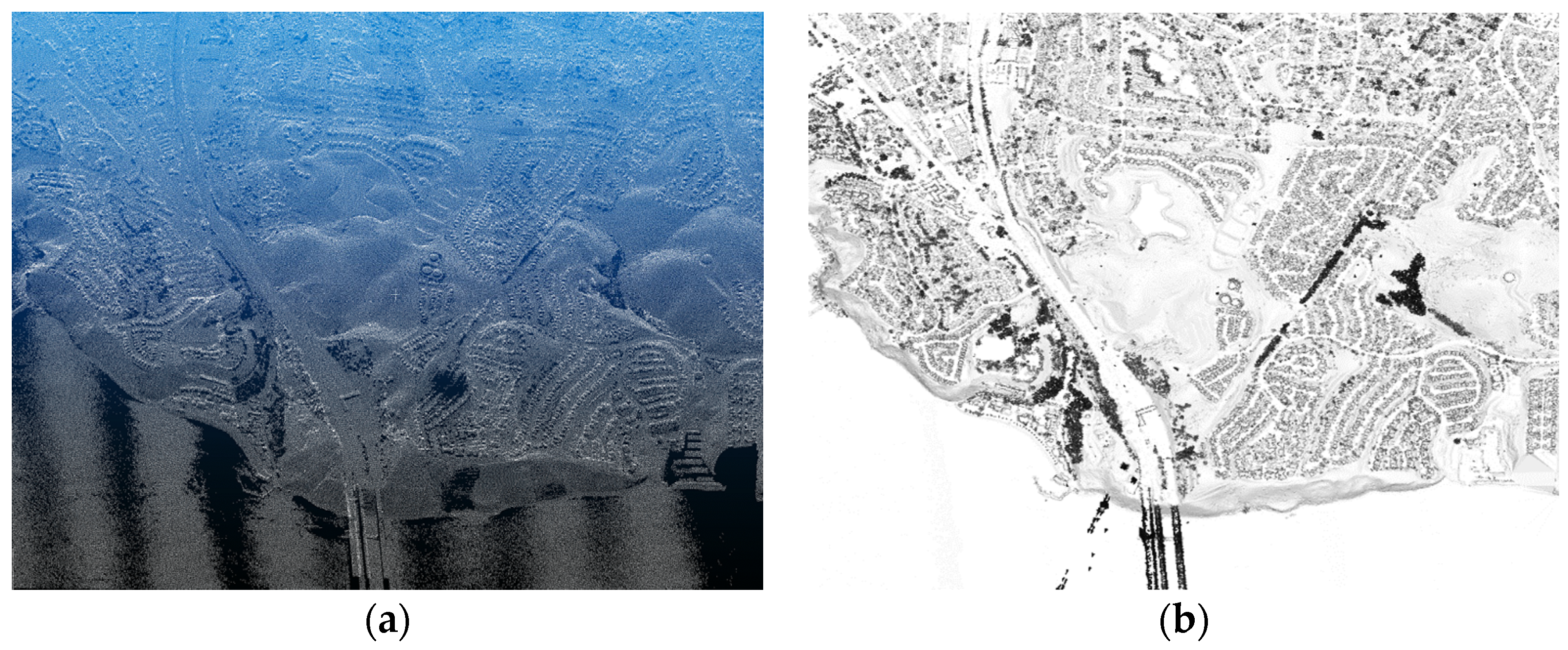
Due to the large scene and dense points of the denoised point cloud data, the direct triangulation will lead to the model file being too large, thus resulting in the memory requirements bottlenecked in the subsequent SAR imaging processing. We resort to down-sampling to solve this problem, and the idea of down-sampling is to check if there is a point in each voxel that can replace the whole. If so, a point is used to replace the point set in the voxel. Here, the average value (centroid) of all point coordinates in each voxel is selected to replace all points. The down-sampled point cloud is shown in Figure 5a.
In order to convert the down-sampled LiDAR point cloud data into a 3D model, we will apply the Delaunay triangulation method. The Delaunay triangulation is a fundamental algorithm in computational geometry that is used to create a triangulation of a given set of points satisfying a specific property called the Delaunay condition. This principle is widely used in various applications such as computer graphics, terrain analysis, and mesh generation. The Delaunay triangulation is a way to divide a set of points into a simplicial complex, which is a collection of triangles that cover the entire point set. The Delaunay condition states that for every triangle in the triangulation, there should be no other point within its circumcircle, which is the circle passing through the three vertices of the triangle.
The Delaunay process begins with three points forming an initial triangle that encompasses all the input points. Then, the remaining points are inserted one by one. When a new point is added, the algorithm determines the triangle(s) that contain the newly inserted point. These triangles are then split into smaller ones by connecting the new point to their vertices. After the insertion, the algorithm checks the local Delaunay condition for each newly created triangle and flips any violated edges until the global Delaunay condition is met. This iterative process continues until all points have been inserted, resulting in the final Delaunay triangulation. As an example, the LiDAR point cloud data on a part of city of Vallejo were converted into a 3D model of the coastal areas by utilizing Delaunay triangulation, as illustrated in Figure 5b.

3.3. SAR Imaging Simulation Based on RaySAR

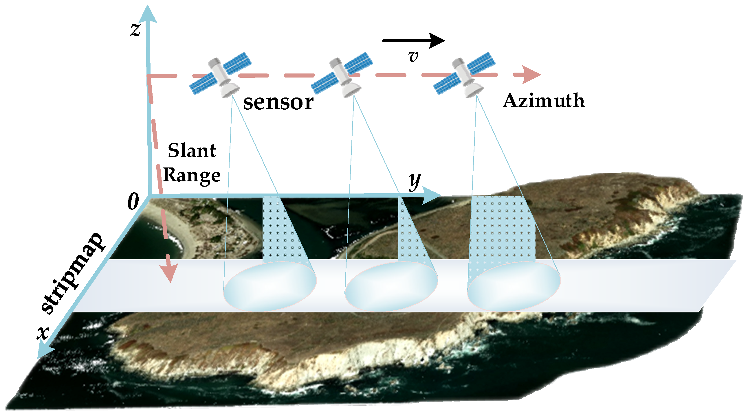
On the basis of the coastal areas modeling aforementioned, SAR imaging simulation can be performed. The schematic of stripmap SAR is depicted in Figure 6. Stripmap mode is the most basic SAR imaging mode, in which the radar antenna remains fixed in a pointing direction. The imaging area is a ground strip parallel to the direction of movement of the radar sensor platform. The width of the imaging band can be changed, ranging from several kilometers to hundreds of kilometers. Our main purpose is to make a comparison between the focused image processed using real SAR raw data and simulated SAR images. Therefore, we will use a SAR simulator for SAR imaging simulation on the basis of our geometrical model built using LiDAR point cloud data.
In order to obtain a high-resolution SAR image, we resorted to RaySAR simulator [27,28] due to its high efficiency and flexibility. RaySAR is a SAR imaging simulator [49] that was developed at the Technical University of Munich in collaboration with the German Aerospace Center (DLR, Institute of Remote Sensing Technology) in Stefan Auer’s doctoral thesis [29]. It can generate ultra-high resolution SAR products. However, for the large number of triangular surface patches in the triangulated 3D coastal areas model, it is not able to be processed directly with the RaySAR for SAR simulation. To solve this problem, we propose to perform SOR denoising and down-sampling processing on the point cloud model before triangulation, so that the model of 3D coastal areas can be utilized by RaySAR. It also avoids mismodeling phenomena such as spikes.
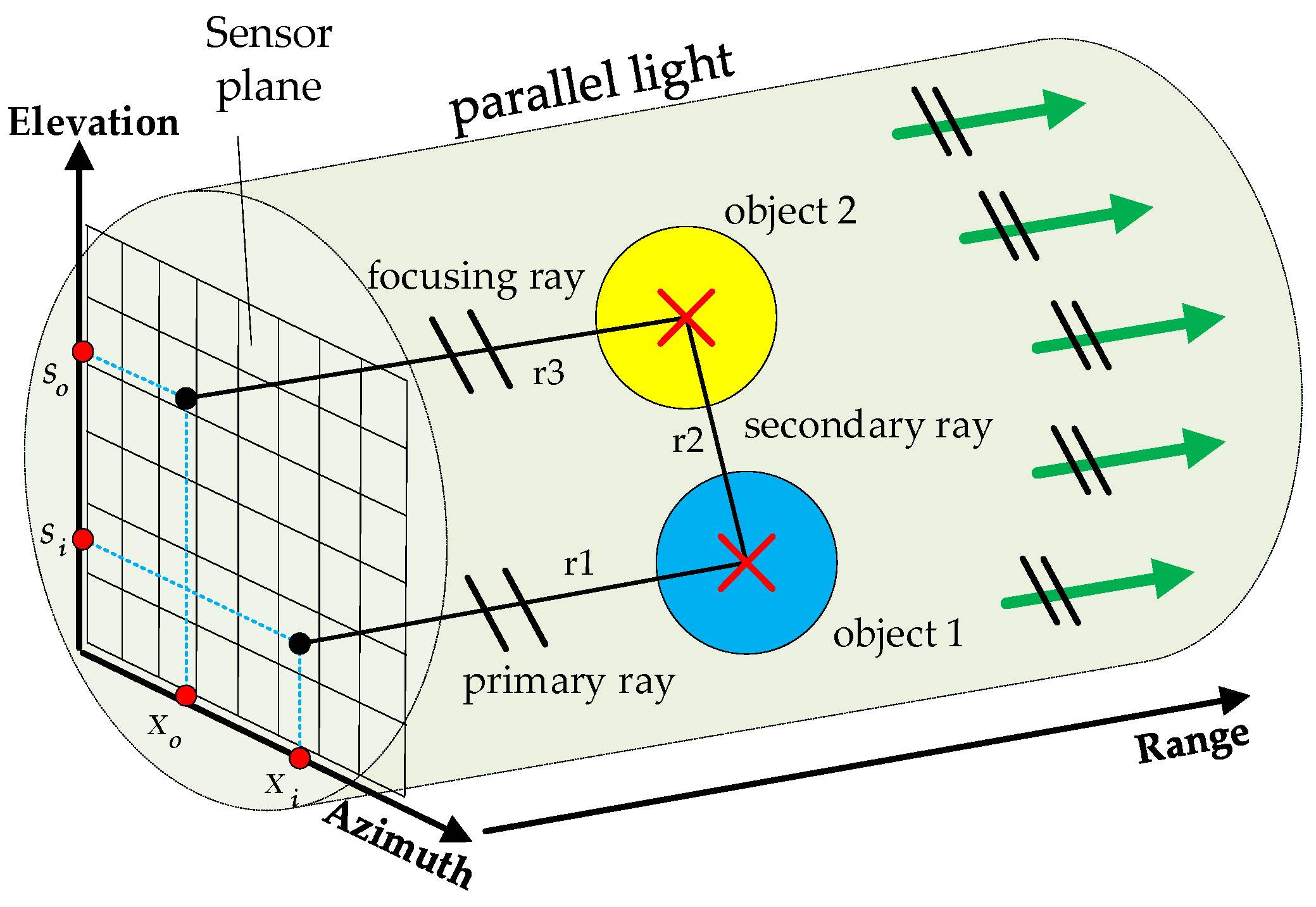
The SAR imaging system of RaySAR is approximated using a cylindrical light source and an orthographic camera. Figure 7 shows a schematic of ray tracing, and the process of double reflection of ray is also described. The reflection contribution is evaluated with the backward ray tracing technique, that is, light starting at the sensor and ending at the signal source. By this way, rays that do not intersect the scene and cannot reach the light source are not traced. Compared with the forward ray tracing, the computational complexity is greatly reduced, and the computational efficiency is improved.
For the final SAR image, the position of each sampling point is determined with one or more intersection points between the ray and the target model. The azimuth position is determined using the average value of the azimuth coordinates of the N intersection points, and the position of the range direction is determined using half the distance traveled by the ray.
For the calculation of the contribution of the signal strength, the initial intensity of the emitted ray is set, and the weight factor is reduced with each bounce. Finally, the contribution of all the bounce times is added up. At each contact with the target surface, the contributions of specular and diffuse reflections are calculated separately. The formula for diffuse reflection contribution is as follows:
I d = k I ( N L ) b
where k is a diffuse reflection factor, and I is intensity of the incoming signal. b is a surface brilliance factor. L is the direction of the intersection point pointing to the light source. N is the normal vector of the target surface at the intersection point. For a specular reflection contribution, the formula is as follows:
I s = s ( N H ) 1 r
where s is a specular reflection coefficient, and r is a roughness factor defining the sharpness of the specular highlight. H is the angular bisector direction of the incident and reflected rays at the intersection point. The whole radiometry contribution can be evaluated through Equations (13) and (14).
From the radiometrical point of view, the RaySAR model for specular reflection is used to approximate the Fresnel reflection model, while the RaySAR model for diffuse reflection is used to approximate the small perturbation method (SPM). Finally, by setting the coefficients of specular reflection and diffuse reflection, the RaySAR model can be used to approximate the common radar model. In contrast to the Fresnel refection model, the angular dependence of the reflection coefficient on the surface permittivity and signal polarization is not considered.
In order to perform SAR imaging of large-scene coastal areas based on RaySAR simulator, we generated the 3000 m × 3000 m large-scene coastal areas model via denoising, down-sampling, and triangulating the LiDAR point cloud data. As an imaging scenario of large-scene coastal areas, the SAR reflectance map is evaluated with backward ray tracing, and the simulated SAR image can be obtained by performing convolution of the reflectance map and the SAR impulse response.
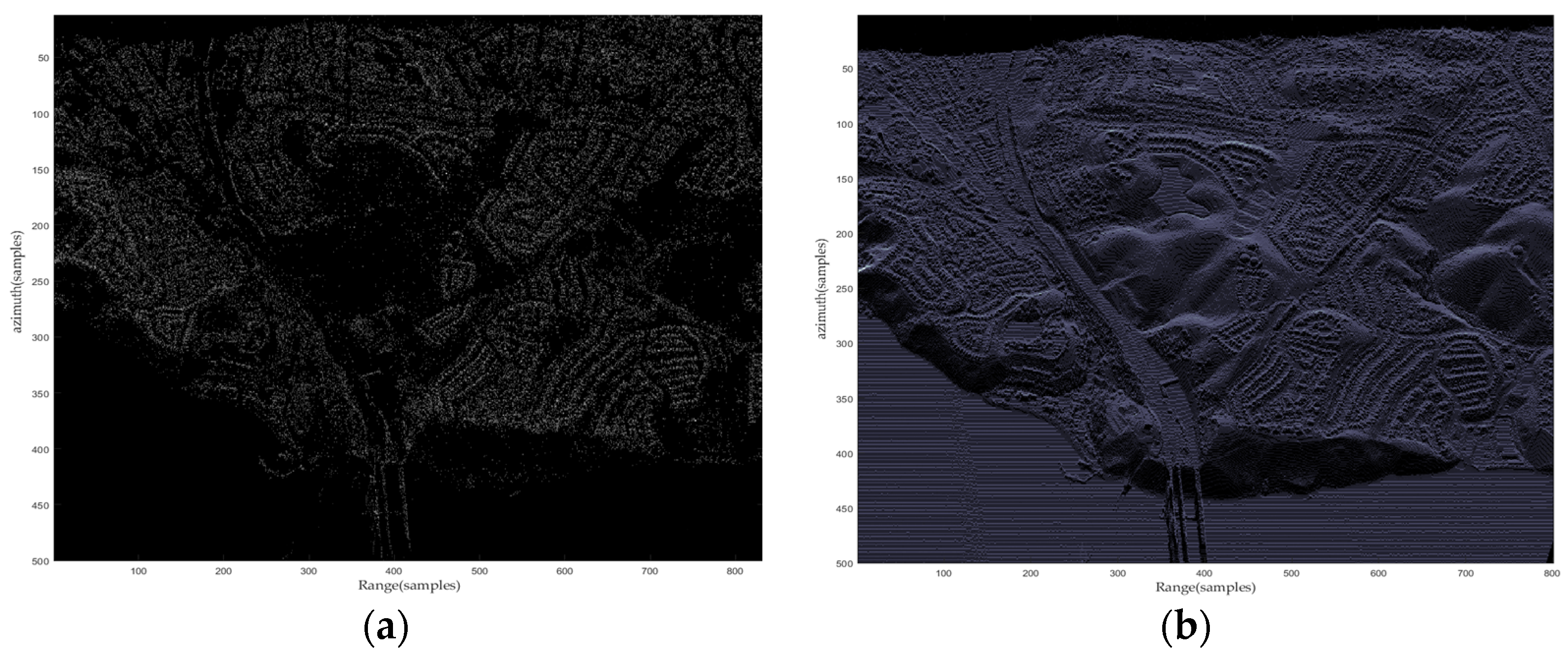
All contributions with the same bounce level will be separated into different layers, and the contribution of only double bounce is shown in Figure 8a. It can be seen from Figure 8a that the double bounce mainly occurs in areas such as buildings and bridges. The first five bounce contributions are superimposed, based on which a simulated SAR image of Vallejo City obtained with RaySAR is generated, as depicted in Figure 8b.

4. Results

In the following, the parallel RD algorithms developed in this paper are utilized for processing and focusing large-scene coastal areas of Sentinel-1 Level-0 raw data. The focused SAR images of Sentinel-1 raw data with parallel RD algorithms are compared with the simulated SAR images obtained with the RaySAR simulator, as well as the corresponding areas of Google Maps. The comparison results show good agreements, which verify the effectiveness of the parallel RD algorithm as well as the RaySAR simulator.

4.1. SAR Imaging of Point Targets

To establish the imaging model, we will perform a SAR imaging simulation of point targets. The squint angle of the simulated radar is zero, and the platform equipped with the antenna scans the ground target in the way of side-looking. The carrier frequency is set to 5 GHz. The bandwidth is set to 200 MHz, and the range sampling rate is set to 320 MHz. The platform carrying the radar is placed at an altitude of 10,000 m above the ground, and it is made to fly in a straight line along the azimuth direction at a speed of 100 m/s. The radar imaging area is set as a rectangle of 200 m × 200 m. The imaging area is (9900 m and 10,100 m) in range direction, and the scope is (−100 m and 100 m) in the azimuth direction. Figure 9a shows the SAR imaging area and the coordinate settings of five-point targets.
The LFM pulse is transmitted and then the echo is received and orthogonally demodulated. By linearly superimposing the echo signals from five-point targets, the echo signal is obtained. The echo signal and the replicated pulse are transformed with the Fourier transform in range direction. The complex conjugate of the replicated pulse is collected and multiplied with the echo signal in the frequency domain. Then, taking the inverse Fourier transform, the range pulse compression is completed.
Due to the presence of range migration, the signal needs to be corrected before it can be compressed in the azimuth direction. Firstly, the signal is transformed into the range-time domain and the azimuth-frequency domain with the Fourier transform in the azimuth direction, which is also called the Range-Doppler domain. In this domain, signals of the same range and different azimuth can be corrected uniformly using sinc interpolation, and the interpolation kernel length is set to 6. After RCMC, the signal with the azimuth matching filter is multiplied and then the azimuth inverse Fourier transform is performed to return the two-dimensional time domain, and the SAR image of point targets can be obtained with the Range-Doppler algorithm. Figure 9b shows the final compression result of the point targets. It is observed that five point targets are focused well, as shown in white dots in Figure 9b.

4.2. SAR Imaging of Sentinel-1 Level-0 Raw Data

In this subsection, the parallel RD algorithm developed in this paper is applied to deal with Sentinel-1 Level-0 raw data, and the whole imaging process is implemented using python. Sentinel-1 is an earth observation satellite of the Global Monitoring for Environment and Security (GMES). It consists of two satellites, Sentinel-1A and Sentinel-1B, both carrying C-band synthetic aperture radar, with an operating frequency of 5.4 GHz. The strip mode pulse repetition interval is 519 μs, and the pulse time width is 44.2 μs. SAR data can be obtained in daytime, night-time, and various weather conditions [43,44,50]. Sentinel-1 data products are mainly Level-0 raw data, Level-1 Single Look Complex (SLC), Level-1 Ground Range Detected (GRD), and Level-2 Ocean (OCN). Level-1 SLC data are single-look-focused data, and Level-1 GRD data are multiple-look-focused data. Level-2 OCN is commonly applied to the ocean. In the process of real SAR raw data processing, the raw data and associated parameters should first be decoded and extracted in accordance with the data row and column storage standards before the imaging process. After getting the raw echo signal, the radar parameters are combined, and the RD algorithm is used for imaging.
In what follows, two scenes of Sentinel-1 Level-0 raw data are chosen to conduct SAR imaging processing. The first scene SAR raw data were obtained with Sentinel-1A scanning in Santos City, Sao Paulo State, Brazil, on 11 June 2023. The geocode for this area is (−23.9448, −46.3304). The second-scene SAR raw data were obtained with Sentinel-1B scanning a port in Galveston County, Houston, USA, on 19 December 2021. The geocode for this area is (29.3937, −94.9646). The selected Sentinel-1 raw data were all HH polarization. The Sentinel-1 level-0 data for the two scenes are downloaded from the Copernicus Public Access Center.
The raw data are formatted and decoded, and the echo signal and related parameters are extracted. The raw echo signals are shown in Figure 10a,b. Figure 10a corresponds to the data of the first scene, with 21,838 sampling points in the range direction and 48,941 sampling points in the azimuth direction. Due to a large amount of data leading to memory shortage, the data block ranging from the 8000th row to the 18,000th row in azimuth direction are selected, in order to save memory requirements. Figure 10b corresponds to the data of the second scene. The sampling points in the range direction are 22,018, and the total sampling points in the azimuth direction are the same as the first scene. Starting from the 2000th azimuth row, the next 10,000 rows of raw echo signal are selected for SAR imaging processing.
The raw echo signal is converted into frequency domain with the Fourier transform in range direction, multiplied by matched filter and then transformed into a time domain using the inverse Fourier transform in range direction to complete range compression. RCMC is then applied, and the corrected signals are shown in Figure 10c,d in the Range-Doppler domain, respectively. The signal after range compression and RCMC appears in the image as bright lines that are perpendicular to the range direction, so the effectiveness of the RCMC process can be determined. Subsequently, the azimuth pulse compression is carried out, and the focused SAR images are shown in Figure 10e and Figure 10f, respectively. The focused SAR images show obvious echo intensity distribution, with the brighter areas being land and the darker areas being sea surface. Meanwhile, the shape of the mountains in Figure 10e as well as the ships on the sea surface in Figure 10f can also be clearly identified.
In order to make a comparison between the focused SAR images and the corresponding areas of Google Maps, two areas corresponding to the imaging areas of Sentinel-1 raw data were captured from Google Maps, as shown in Figure 11b and Figure 12b, respectively. By comparing the focused SAR image with the corresponding areas of Google Maps, it can be seen from Figure 11a,b that the focused SAR image is in good agreement with Google Maps. The position of the coastal contour line and the direction of the mountain are basically consistent, and the shape of the inland waterway of Santos City is also quite consistent. Similarly, by comparing Figure 12a,b, it can be observed that the focused SAR image is also in good agreement with Google Maps. The elongated geographic shape of Galveston Island in the two images is highly consistent.

4.3. SAR Image Slicing and Enhancement

In order to make a more detailed comparison of the local areas of interest in the focused SAR image, the focused SAR image is sliced first. As local areas of interest, the areas of sampling points in range direction [7500, 9000] and azimuth direction [2700, 4500] are sliced from Figure 10e, as depicted in Figure 13a. The area of the sliced SAR image is about one fiftieth of that of the focused SAR image. Figure 13a,c show a comparison between the sliced SAR image and the Google Maps of the port in Santos City. The unique geographical structure of the port of Santos city in the sliced SAR image can be observed, which coincides with the corresponding areas of Google Maps. Similarly, the areas of sampling points in range direction [13, 250, 15, 250] and azimuth direction [5000, 7000] are sliced from Figure 10f, as shown in Figure 14a. In Figure 14a,c, a comparison is made between SAR sliced images and Google Maps on Galveston Island. The shape of Galveston Island and the location of bridges in SAR slice images in Figure 14a are basically consistent with the corresponding areas of Google Maps as in Figure 14c.
However, the sliced SAR images in Figure 13a and Figure 14a are slightly blurred, and the details such as the main road and the land edge are difficult to identify. Therefore, image enhancement technology is applied to increase the contrast between the strong and weak reflection points in SAR image, to optimize the definition of the sea and land contour, and then to brighten the image. Hence, the local SAR image after magnification is still clear. Figure 13b and Figure 14b are the sliced SAR images after enhancement. From Figure 13 and Figure 14, the effect of SAR image enhancement can be observed. By comparing the sliced SAR image and the corresponding areas of Google Maps, the results show much better agreement after image enhancement.

4.4. Full Imaging Processing for A Large Scene

In Section 3.2, only a part of raw data of a full large scene was extracted and processed, due to the memory requirements. The reason why we do not process all the raw data in a full large scene is that processing the raw data requires large memory, but the device memory we use is 32 GB.
In order to solve this problem, a scheme of dividing the whole data into blocks is presented, as illustrated in Figure 15. Each sub-block of raw data is processed in turn, and the focused SAR images of each sub-block are then merged into a complete SAR image. However, the “folding” phenomenon often occurs in SAR imaging, where various terrain features on the top of the SAR image are overlaid on the bottom, and the terrain on the left side of the image is overlaid on the right side. This problem leads directly to obvious “folding” traces at the connection between blocks after image merging. Therefore, a method is presented here, which can not only solve the trouble caused by the hardware bottleneck but can also avoid the impact of the “folding” phenomenon. Firstly, all the raw data are divided into several sub-blocks in terms of the azimuth direction sampling points, and a certain overlap area is retained between each sub-data block. Each sub-data block is processed into a SAR image. The needed portion of data blocks in blue is reserved, while the overlap area in pink is removed, as depicted in Figure 15.
As an example, our scheme is applied to process the whole raw data of a full large scene, in which the raw data were obtained from the Sentinel-1A satellite scanning of Houston city and surrounding areas on 31 March 2023. The geocode for this area is (29.7805, −95.3863). The scanning area is specifically depicted in the red box in Figure 16a. The total number of azimuth sampling points in the raw data is more than 40,000. We divide the whole raw data into six blocks, and each sub-data block has 9000 azimuth sampling points, in which the area of 1000 azimuth sampling points is set as overlapping part of adjacent sub-data blocks. The six sub-data blocks are processed into SAR image separately, and the overlapping part is removed. Finally, the focused SAR image of the complete scene can be obtained by merging each SAR image corresponding to sub-block raw data, as shown in Figure 16b. In this image, Houston city, of 1440 square kilometers, is shown in the middle of the SAR image, with many of the waterways, roads, and wheat fields around the city easily recognizable. The outline of Lake Conroe can also be readily observed at the bottom of the SAR image.

4.5. Comparison among Sentinel-1 Focused Images, Simulated SAR Image and Google Maps

In Figure 17, a comparison is made among Sentinel-1 focused images, simulated SAR image, and Google Maps. Figure 17a is a simulated SAR image of coastal areas of Vallejo City, and the corresponding areas of Google Maps are shown in Figure 17d. By comparing Figure 17a with Figure 17d, the simulated SAR images show good agreement with the corresponding areas of Google Maps, which demonstrate the effectiveness of SAR imaging simulation procedure including our approach to model realistic coastal areas. In order to compare with the simulated coastal areas SAR images, Sentinel-1 raw data for the corresponding areas of Vallejo City are selected, which were acquired at 14:23 on 5 December 2014, and the polarization mode was VV polarization. The geocoding of the selected area is (38.1010, −122.2550). Sentinel-1 raw data can be downloaded from the Copernicus Public Access Center. The focused SAR images can be obtained using parallel RD algorithm.
After slicing and enhancement, the focused SAR image of the area of the city of Vallejo is shown in Figure 17b, which serves as a real SAR image that can be used for comparison with the simulated SAR image. By comparing Figure 17a and Figure 17b, the simulated SAR images obtained with the RaySAR simulator are in good agreement with the focused SAR image of the area of the city of Vallejo. In Figure 17a,b, the coast contours are consistent, and the bridges located at the bottom central position of the two images are also consistent. It should be noted that a slight difference between Figure 17a and Figure 17b can be seen, which is attributed to the different relative positions of the sensors, the scene center in the simulation and the actual situation. In our simulation of SAR imaging, the point cloud model of the real ground object is obtained via LiDAR scanning. Hence, the SAR imaging simulator with high flexibility can serve as a supplement for the detail scattering information of the real SAR image.
In addition, Sentinel Application Platform (SNAP), as a common architecture for all Sentinel Toolboxes, was used to preprocess and multiple-look process the level-1 data of the selected area in our study. The processing result using SNAP software is shown in Figure 17c. The SAR image obtained with SNAP software is relatively clear, mainly due to preprocessing as well as multi-look processing. From Figure 17b,c, the focused SAR image with our parallel RD algorithm is in good agreement with the multi-look SAR image processed using SNAP software.

5. Discussion

5.1. Quality Evaluation of Reconstructed Images

In order to numerically evaluate reconstructed images, the cosine similarity between the simulated image and real image is defined as follows [51]:
C ( f , g ) = f T g f 2 g 2
where f is the feature vector of the first image, and g is that of the second image. 2 represents the vector’s Euclidean norm. Cosine similarity C ( f , g ) indicates that the bigger the similarity C ( f , g ) is, the greater the correlation is between two images. The cosine similarity C ( f , g ) ranges from [0, 1], and the larger the value, the more similar it is.
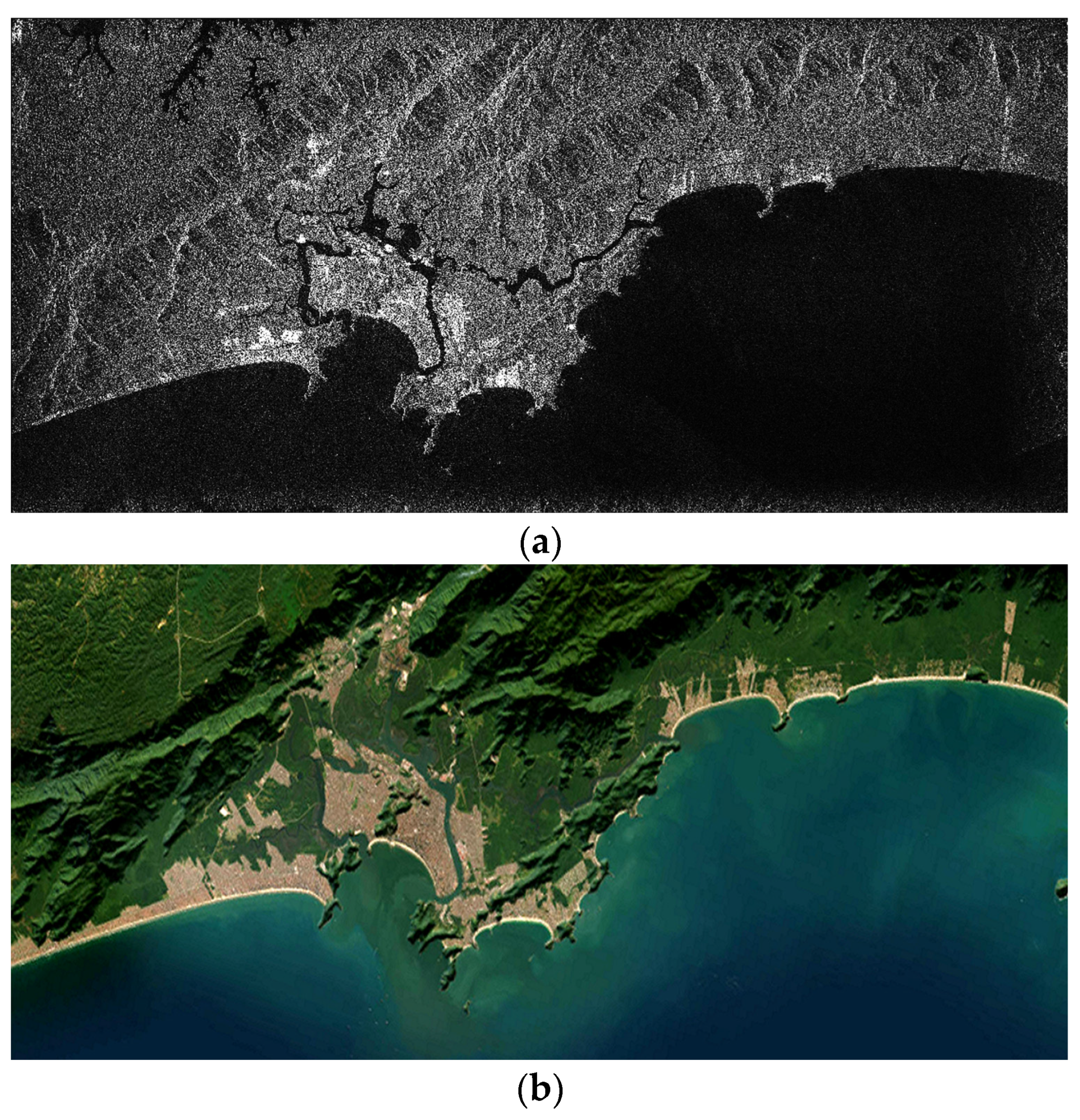
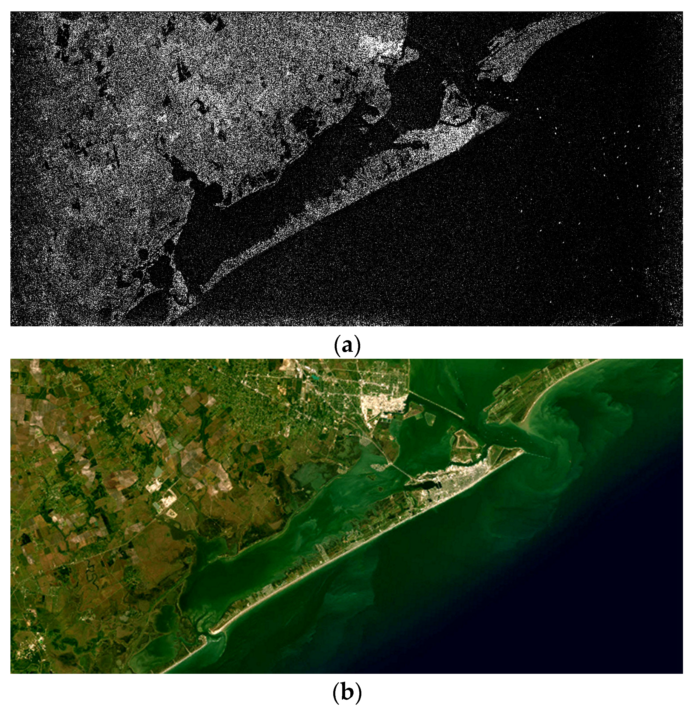
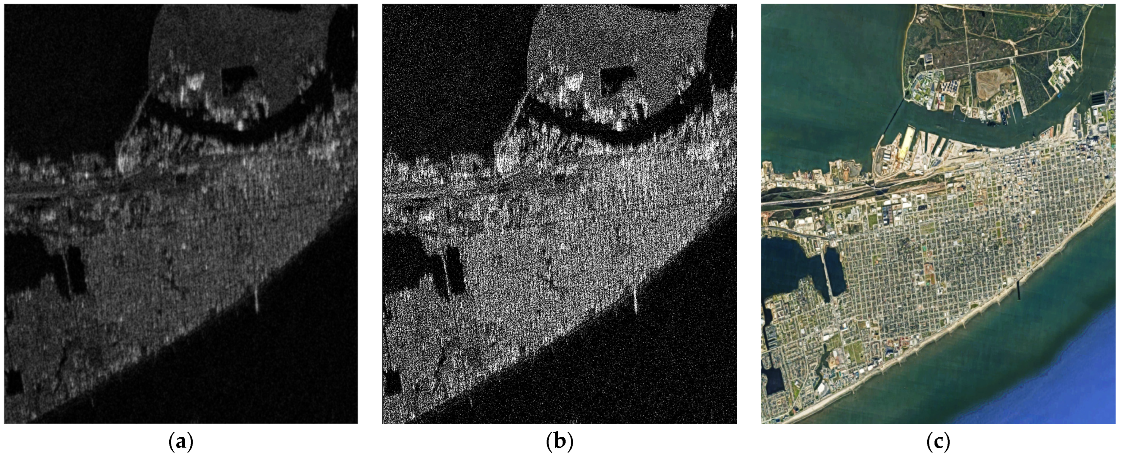
Using Equation (15), the cosine similarity between Sentinel-1 SAR-focused images as in Figure 17b and multi-look SAR images processed with SNAP software as in Figure 17c is 0.85. The comparison indicates a satisfactory similarity between Sentinel-1-focused SAR images using our parallel RD algorithm and multi-look SAR image processed using SNAP software, which proves the effectiveness of our parallel RD algorithm for focusing the Sentinel-1 raw data. The cosine similarity reaches 0.93 between the simulated SAR image with RaySAR simulator as in Figure 17a and the corresponding areas of Google Maps as in Figure 17d. In addition, by comparing Sentinel-1 SAR-focused images with our parallel RD algorithm as in Figure 17b and RaySAR-simulated SAR image as in Figure 17a, a cosine similarity of 0.81 was obtained. This is due mainly to the rotational angle deviation between our focused SAR image and Google Maps.

5.2. Parallel Scheme of RD Algorithm

As we know, the SAR imaging system can be regarded as a linear system, and SAR-focused imaging of level-0 raw data has natural advantages of parallel processing, due to its “stop-go-stop” operating mode. Hence, in this study, a CPU parallel scheme of Range-Doppler (RD) is proposed to focus Sentinel-1 level-0 raw data due to the fact that Sentinel-1 level-0 raw data can be divided into several separate blocks, provided that CPU cores are sufficient. Moreover, the speedup ratio is almost linear proportional to CPU cores. Although the parallel RD algorithm based on CPU is not novel, the scheme is simple and easy to implement. Many acceleration algorithms have been proposed over the last decade and nowadays, but most of these acceleration algorithms are devoted to accelerating algorithm itself, which is complex and not easy to implement.
Taking the workstation (CPU: 20 cores, Intel(R) Xeon(R) Silver 4114 CPU @ 2.20 GHz) used in this study for example, almost 20× speedup ratio was achieved. In our future research, the parallel techniques of the CPU–GPU heterogeneous architecture are under consideration for focusing a large amount of Sentinel-1 level-0 raw data.

5.3. Limitations of This Work

The accuracy of SAR imaging simulations heavily depends on the quality of input data and the assumptions made during the simulation process. Any inaccuracies in the input data or simulation assumptions can affect the reliability of the results. In general, the geometrical model cannot fully represent the complexity of real-world scenes, which can include various types of terrain and objects with different scattering properties.
While this work proposes a scheme for converting LiDAR point cloud data into a 3D coastal area DEM, it may oversimplify the complexities involved in LiDAR data processing. LiDAR data can be noisy, and various preprocessing steps are often required to obtain an accurate 3D model.
The study does not extensively discuss the uncertainty associated with SAR imaging, simulation, and modeling. Real-world SAR data can be affected by noise, atmospheric conditions, and other factors that introduce uncertainties into the results.
The efficiency of the parallel RD algorithm is highlighted, but the computational resources required for these processes may not be readily available in all research or operational settings.

6. Conclusions

In this paper, a parallel RD algorithm is developed for improving the efficiency of large-scene SAR imaging of SAR raw data. The scheme of parallel RD algorithm is first presented, and its validity is verified by performing SAR imaging simulation for ideal points target. The parallel RD algorithm is then applied to focus SAR raw data decoded from the latest Sentinel-1 data for large coastal scene, and the focused SAR images of large coastal scene are in good accordance with Google Maps. Due to its high efficiency and flexibility, the RaySAR simulator based on ray tracing method is utilized in this paper for SAR imaging simulation of large coastal scene, which is modeled using LiDAR point cloud data. Because of the large number of triangular surface patches in the triangulated 3D coastal area models, we propose to perform SOR denoising and down-sampling processing on the point cloud model before triangulation, the tailored model of 3D coastal areas suitable for RaySAR simulator. In order to make a comprehensive comparison, the simulated SAR image of a selected 3D coastal area is compared with a focused SAR image of Sentinel-1 data, the multi-look-processed SAR image using SNAP software, as well as the corresponding areas of Google Maps. The comparison results show good agreements, which verify the effectiveness of the parallel RD algorithm as well as the RaySAR simulator. In addition, slicing and enhancing techniques are applied to zoom in on any region of interest, which are still clearly visible. Using a comprehensive study that involves various components, including Sentinel-1 raw data, SAR imaging simulation, and Google Maps, this comparative analysis allows for the assessment of the developed algorithm’s performance and accuracy, providing valuable references for researchers and engineers in related fields of SAR imaging research and applications. In the future, a more reasonable electromagnetic simulator will be developed for SAR imaging simulation, in which the scattering from large-scale facets as well as small-scale structure will be taken into account by PO and SPM, respectively, along with ray tracing techniques.

Author Contributions

Methodology, H.J. and P.Y.; software, H.J.; validation, H.J.; formal analysis, H.J.; ray tracing simulation, R.W.; investigation, H.J. and P.Y.; resources, P.Y.; writing—original draft preparation, H.J.; writing—review and editing, P.Y.; visualization, H.J.; supervision, P.Y.; project administration, H.J. and P.Y. All authors have read and agreed to the published version of the manuscript.

Funding

This work was supported in part by the National Natural Science Foundation of China [Grant Nos. 62061048, 62261054, 61961041, and 62361054], in part by the Shaanxi Key Research and Development Program [Grant No. 2023-YBGY-254], and in part by the Natural Science Foundation of the Educational Department of Shaanxi Province (Grant No 18JK0872).

Data Availability Statement

We used the Sentinel-1 raw data from https://search.asf.alaska.edu/, as well as LiDAR point cloud data from https://opentopography.org/. Google Maps is used in this study for a comparison, and its copyrights belongs to the Google company, registered in California, USA.

Acknowledgments

The authors sincerely thank the Sentinel-1 open data products provided by the European Space Agency (ESA), the RaySAR simulator provided by Stefan Auer, the LiDAR point cloud data provided by OpenTopography, and the anonymous reviewers for their valuable comments and enlightenment.

Conflicts of Interest

The authors declare no conflict of interest.

Abbreviations

The following abbreviations are used in this manuscript:
RDRange-Doppler
SARSynthetic Aperture Radar
JPLJet Propulsion Laboratory
RCMCRange Cell Migration Correction
SRCSecond Range Compression
CADComputer-Aided Design
BARTBidirectional Analytic Ray Tracing
LiDARLight Detection and Ranging
DEMDigital Elevation Model
TOPSTerrain Observation by Progressive Scans
FFTFast Fourier transform
SORStatistical Outlier Removal
GMESGlobal Monitoring for Environment and Security
SPMSmall Perturbation Method
SLCSingle-Look Complex
GRDGround Range Detected
OCNOcean
SNAPSentinel Application Platform
DLRGerman Aerospace Center

References

  1. Xing, M.; Jiang, X.; Wu, R.; Zhou, F.; Bao, Z. Motion compensation for UAV SAR based on raw radar data. IEEE Trans. Geosci. Remote Sens. 2009, 47, 2870–2883. [Google Scholar] [CrossRef]
  2. Zhang, L.; Xing, M.; Qiu, C.W.; Li, J.; Sheng, J.; Li, Y.; Bao, Z. Resolution enhancement for inversed synthetic aperture radar imaging under low SNR via improved compressive sensing. IEEE Trans. Geosci. Remote Sens. 2010, 48, 3824–3838. [Google Scholar] [CrossRef]
  3. Xing, M.; Wu, Y.; Zhang, Y.D.; Sun, G.C.; Bao, Z. Azimuth resampling processing for highly squinted synthetic aperture radar imaging with several modes. IEEE Trans. Geosci. Remote Sens. 2013, 52, 4339–4352. [Google Scholar] [CrossRef]
  4. Zhao, Y.; Zhang, M.; Zhao, Y.W.; Geng, X.P. A bistatic SAR image intensity model for the composite ship–ocean scene. IEEE Trans. Geosci. Remote Sens. 2015, 53, 4250–4258. [Google Scholar] [CrossRef]
  5. Lazarov, A. SAR signal formation and image reconstruction of a moving sea target. Electronics 2022, 11, 1999. [Google Scholar] [CrossRef]
  6. Giudici, D.; Mancon, S.; Guarnieri, A.M.; Piantanida, R.; Prandi, G.; Recchia, L.; Recchia, A. Enhanced processing of Sentinel-1 TOPSAR data. In Proceedings of the 2016 IEEE International Geoscience and Remote Sensing Symposium (IGARSS), Beijing, China, 10–15 July 2016; pp. 5019–5022. [Google Scholar]
  7. Moreira, A.; Prats-Iraola, P.; Younis, M.; Krieger, G.; Hajnsek, I.; Papathanassiou, K.P. A tutorial on synthetic aperture radar. IEEE Geosci. Remote Sens. Mag. 2013, 1, 6–43. [Google Scholar] [CrossRef]
  8. Mittermayer, J.; Kraus, T.; López-Dekker, P.; Prats-Iraola, P.; Krieger, G.; Moreira, A. Wrapped staring spotlight SAR. IEEE Trans. Geosci. Remote Sens. 2016, 54, 5745–5764. [Google Scholar] [CrossRef]
  9. Zhang, M.; Zhou, P.; Zhang, X.; Dai, Y.; Sun, W. Space-variant analysis and target echo simulation of geosynchronous SAR. J. Eng. 2019, 2019, 5652–5656. [Google Scholar] [CrossRef]
  10. Xie, Y.; Zeng, H.; Yang, K.; Yuan, Q.; Yang, C. Water-body detection in Sentinel-1 SAR images with DK-CO network. Electronics 2023, 12, 3163. [Google Scholar] [CrossRef]
  11. Huang, M.; Liu, Z.; Liu, T.; Wang, J. CCDS-YOLO: Multi-category synthetic aperture radar image object detection model based on YOLOv5s. Electronics 2023, 12, 3497. [Google Scholar] [CrossRef]
  12. Tsokas, A.; Rysz, M.; Pardalos, P.M.; Dipple, K. SAR data applications in earth observation: An overview. Expert Syst. Appl. 2022, 205, 117342. [Google Scholar] [CrossRef]
  13. Zhang, F.; Yao, X.; Tang, H.; Yin, Q.; Hu, Y.; Lei, B. Multiple mode SAR raw data simulation and parallel acceleration for Gaofen-3 mission. IEEE J. Sel. Top. Appl. Earth Obs. Remote Sens. 2018, 11, 2115–2126. [Google Scholar] [CrossRef]
  14. Xu, P.; Wang, Y.; Xu, X.; Wang, L.; Wang, Z.; Yu, K.; Wu, W.; Wang, M.; Leng, G.; Ge, D. Structural-electromagnetic-thermal coupling technology for active phased array antenna. Int. J. Antennas Propag. 2023, 2023, 2843443. [Google Scholar] [CrossRef]
  15. Fan, W.; Zhang, M.; Li, J.; Wei, P. Modified Range-Doppler algorithm for high squint SAR echo processing. IEEE Geosci. Remote Sens. Lett. 2018, 16, 422–426. [Google Scholar] [CrossRef]
  16. Cao, R.; Wang, Y.; Sun, S.; Zhang, Y. Three dimension airborne SAR imaging of rotational target with single antenna and performance analysis. IEEE Trans. Geosci. Remote Sens. 2022, 60, 5225417. [Google Scholar] [CrossRef]
  17. Wang, Z.; Wei, F.; Huang, Y.; Zhang, X.; Zhang, Z. Improved RD imaging method based on the principle of step-by-step calculation. In Proceedings of the 2021 2nd China International SAR Symposium (CISS), Shanghai, China, 3–5 November 2021; pp. 1–5. [Google Scholar]
  18. Huang, P.; Xu, W. An efficient imaging approach for TOPS SAR data focusing based on scaled Fourier transform. Prog. Electromagn. Res. B 2013, 47, 297–313. [Google Scholar] [CrossRef]
  19. Zhang, S.X.; Xing, M.D.; Xia, X.G.; Zhang, L.; Guo, R.; Bao, Z. Focus improvement of high-squint SAR based on azimuth dependence of quadratic range cell migration correction. IEEE Geosci. Remote Sens. Lett. 2012, 10, 150–154. [Google Scholar] [CrossRef]
  20. Dai, C.; Zhang, X.; Shi, J. Range cell migration correction for bistatic SAR image formation. IEEE Geosci. Remote Sens. Lett. 2011, 9, 124–128. [Google Scholar] [CrossRef]
  21. Jin, M.Y.; Wu, C. A SAR correlation algorithm which accommodates large-range migration. IEEE Trans. Geosci. Remote Sens. 1984, GE-22, 592–597. [Google Scholar] [CrossRef]
  22. Wang, G.; Zhang, L.; Hu, Q. A novel range cell migration correction algorithm for highly squinted SAR imaging. In Proceedings of the 2016 CIE International Conference on Radar (RADAR), Guangzhou, China, 10–13 October 2016; pp. 1–4. [Google Scholar]
  23. Ding, Z.; Zheng, P.; Li, H.; Zhang, T.; Li, Z. Spaceborne high-squint high-resolution SAR imaging based on two-dimensional spatial-variant range cell migration correction. IEEE Trans. Geosci. Remote Sens. 2022, 60, 5240114. [Google Scholar] [CrossRef]
  24. Xiao, J.; Hu, X.C. A modified RD algorithm for airborne high squint mode SAR imaging. In Proceedings of the 2007 1st Asian and Pacific Conference on Synthetic Aperture Radar, Huangshan, China, 5–9 November 2007; pp. 444–448. [Google Scholar]
  25. Xu, F.; Jin, Y.Q. Mapping and projection algorithm: A new approach to SAR imaging simulation for comprehensive terrain scene. In Proceedings of the 2006 IEEE International Symposium on Geoscience and Remote Sensing, Denver, CO, USA, 31 July–4 August 2006; pp. 399–402. [Google Scholar]
  26. Margarit, G.; Mallorqui, J.J.; Rius, J.M.; Sanz-Marcos, J. On the usage of GRECOSAR, an orbital polarimetric SAR simulator of complex targets, to vessel classification studies. IEEE Trans. Geosci. Remote Sens. 2006, 44, 3517–3526. [Google Scholar] [CrossRef]
  27. Auer, S.; Hinz, S.; Bamler, R. Ray tracing for simulating reflection phenomena in SAR images. In Proceedings of the IGARSS 2008—2008 IEEE International Geoscience and Remote Sensing Symposium, Boston, MA, USA, 7–11 July 2008; pp. V-518–V-521. [Google Scholar]
  28. Auer, S.; Hinz, S.; Bamler, R. Ray-tracing simulation techniques for understanding high-resolution SAR images. IEEE Trans. Geosci. Remote Sens. 2009, 48, 1445–1456. [Google Scholar] [CrossRef]
  29. Auer, S.J. 3D Synthetic Aperture Radar Simulation for Interpreting Complex Urban Reflection Scenarios. Ph.D. Thesis, Technische Universität München, Munich, Germany, 2011. [Google Scholar]
  30. Auer, S.; Gernhardt, S.; Bamler, R. Ghost persistent scatterers related to multiple signal reflections. IEEE Geosci. Remote Sens. Lett. 2011, 8, 919–923. [Google Scholar] [CrossRef]
  31. Auer, S.; Gernhardt, S. Linear signatures in urban SAR images—Partly misinterpreted? IEEE Geosci. Remote Sens. Lett. 2014, 11, 1762–1766. [Google Scholar] [CrossRef]
  32. Tao, J.; Auer, S.; Palubinskas, G.; Reinartz, P.; Bamler, R. Automatic SAR simulation technique for object identification in complex urban scenarios. IEEE J. Sel. Top. Appl. Earth Obs. Remote Sens. 2013, 7, 994–1003. [Google Scholar] [CrossRef]
  33. Placidi, S.; Vetere, A.; Pino, E.; Meta, A. KAISAR: Physics-based GPU-accelerated realistic SAR Simulator. In Proceedings of the EUSAR 2022; 14th European Conference on Synthetic Aperture Radar, Leipzig, Germany, 25–27 July 2022; pp. 1–6. [Google Scholar]
  34. Xu, F.; Jin, Y.Q. Bidirectional analytic ray tracing for fast computation of composite scattering from electric-large target over a randomly rough surface. IEEE Trans. Antennas Propag. 2009, 57, 1495–1505. [Google Scholar] [CrossRef]
  35. Dong, C.L.; Guo, L.X.; Meng, X. An accelerated algorithm based on GO-PO/PTD and CWMFSM for EM scattering from the ship over a sea surface and SAR image formation. IEEE Trans. Antennas Propag. 2020, 68, 3934–3944. [Google Scholar] [CrossRef]
  36. Behera, H.S.; Ramiya, A.M. Urban flood modelling simulation with 3D building models from airborne LiDAR point cloud. In Proceedings of the 2022 IEEE Mediterranean and Middle-East Geoscience and Remote Sensing Symposium (M2GARSS), Istanbul, Turkey, 7–9 March 2022; pp. 145–148. [Google Scholar]
  37. Liu, B.; Bi, X.; Gu, L. 3D point cloud construction and display based on LiDAR. In Proceedings of the 2022 2nd International Conference on Computer, Control and Robotics (ICCCR), Shanghai, China, 18–20 March 2022; pp. 268–272. [Google Scholar]
  38. Chen, S.Y.; Chang, S.F.; Yang, C.W. Generate 3D triangular meshes from spliced point clouds with cloudcompare. In Proceedings of the 2021 IEEE 3rd Eurasia Conference on IOT, Communication and Engineering (ECICE), Yunlin, Taiwan, 29–31 October 2021; pp. 72–76. [Google Scholar]
  39. Elaksher, A.F.; Bethel, J.S. Reconstructing 3D buildings from LiDAR data. Int. Arch. Photogramm. Remote Sens. Spat. Inf. Sci. 2002, 34, 102–107. [Google Scholar]
  40. Zhang, Y.; Xiang, S.; Wan, Y.; Cao, H.; Luo, Y.; Zheng, Z. DEM extraction from airborne LiDAR point cloud in thick-forested areas via convolutional neural network. In Proceedings of the IGARSS 2020-2020 IEEE International Geoscience and Remote Sensing Symposium, Waikoloa, HI, USA, 26 September–2 October 2020; pp. 461–464. [Google Scholar]
  41. Yao, S.; Shi, J. Road 3D point cloud data modeling based on LiDAR. In Proceedings of the 2022 4th International Conference on Intelligent Control, Measurement and Signal Processing (ICMSP), Hangzhou, China, 8–10 July 2022; pp. 465–468. [Google Scholar]
  42. Potin, P.; Rosich, B.; Miranda, N.; Grimont, P.; Shurmer, I.; O’Connell, A.; Krassenburg, M.; Gratadour, J.B. Copernicus Sentinel-1 constellation mission operations status. In Proceedings of the IGARSS 2019—2019 IEEE international geoscience and remote sensing symposium, Yokohama, Japan, 28 July–2 August 2019; pp. 5385–5388. [Google Scholar]
  43. Kirkove, M.; Orban, A.; Derauw, D.; Barbier, C. A TOPSAR processor based on the Omega-K algorithm: Evaluation with Sentinel-1 data. In Proceedings of the Proceedings of EUSAR 2016: 11th European Conference on Synthetic Aperture Radar, Hamburg, Germany, 6–9 June 2016; pp. 1–5. [Google Scholar]
  44. Kim, K.; Kim, J.H. Analysis of Sentinel-1 TOPSAR raw data for synthesizing single look complex image. In Proceedings of the 2021 IEEE International Geoscience and Remote Sensing Symposium IGARSS, Brussels, Belgium, 11–16 July 2021; pp. 3944–3947. [Google Scholar]
  45. Wang, J.; Wen, Y.; Wang, W.; Guo, Z. Research of sidelobe suppression of RDA and CSA imaging algorithms. In Proceedings of the 2015 IEEE International Conference on Signal Processing, Communications and Computing (ICSPCC), Ningbo, China, 19–22 September 2015; pp. 1–5. [Google Scholar]
  46. Jiang, N.; Zhu, J.; Feng, D.; Xie, Z.; Wang, J.; Huang, X. High-resolution SAR Imaging with azimuth missing data based on sub-echo segmentation and reconstruction. Remote Sens. 2023, 15, 2428. [Google Scholar] [CrossRef]
  47. Sofiani, R.; Heidar, H.; Kazerooni, M. An efficient raw data simulation algorithm for large complex marine targets and extended sea clutter in spotlight SAR. Microw. Opt. Technol. Lett. 2018, 60, 1223–1230. [Google Scholar] [CrossRef]
  48. Sun, G.; Xing, M.; Wang, Y.; Wu, Y.; Wu, Y.; Bao, Z. Sliding spotlight and TOPS SAR data processing without subaperture. IEEE Geosci. Remote Sens. Lett. 2011, 8, 1036–1040. [Google Scholar] [CrossRef]
  49. Balz, T.; Hammer, H.; Auer, S. Potentials and limitations of SAR image simulators–A comparative study of three simulation approaches. ISPRS J. Photogramm. Remote Sens. 2015, 101, 102–109. [Google Scholar] [CrossRef]
  50. Fusco, A.; Pepe, A.; Lanari, R. Sentinel-1 TOPS data focusing based on a modified two-step processing approach. In Proceedings of the 2017 IEEE International Geoscience and Remote Sensing Symposium (IGARSS), Fort Worth, TX, USA, 23–28 July 2017; pp. 2389–2391. [Google Scholar]
  51. Jakhetiya, V.; Chaudhary, S.; Subudhi, B.N.; Lin, W.; Guntuku, S.C. Perceptually unimportant information reduction and Cosine similarity-based quality assessment of 3D-synthesized images. IEEE Trans. Image Process. 2022, 31, 2027–2039. [Google Scholar]
Figure 1. Flow chart of the parallel scheme for block processing on large amount data.
Electronics 12 04312 g001
Figure 2. Block diagram of a comprehensive comparative study for coastal areas.
Electronics 12 04312 g002
Figure 3. Flow chart of the approach to modeling the 3D coastal areas.
Electronics 12 04312 g003
Figure 4. Coastal areas LiDAR point cloud data: (a) the original point cloud data; (b) the point cloud data after denoising.
Electronics 12 04312 g004
Figure 5. Three-dimensional model of the coastal areas: (a) LiDAR point cloud after down-sampling; (b) 3D model of the coastal areas after Delaunay triangulation.
Electronics 12 04312 g005
Figure 6. Schematic of spaceborne SAR imaging simulation in coastal areas.
Electronics 12 04312 g006
Figure 7. SAR ray simulation in a hypothetical scene.
Electronics 12 04312 g007
Figure 8. Simulated SAR image of coastal areas of Vallejo City obtained with RaySAR: (a) simulated SAR image with double bounce contributions; (b) simulated SAR image with first five bounce contributions.
Electronics 12 04312 g008
Figure 9. Point target model and imaging results: (a) imaging area and point target position; (b) the focused SAR image of point targets.
Electronics 12 04312 g009
Figure 10. SAR imaging for two scenes of Sentinel-1 level-0 raw data. (a,b) Raw echoes for the first and second scenes, respectively; (c,d) raw echoes after range pulse compression and range migration correction for the first and second scenes, respectively; and (e,f) the focused SAR images for the first and second scenes, respectively.
Electronics 12 04312 g010
Figure 11. Comparison between the focused SAR image for the first scene and the corresponding areas of Google Maps: (a) SAR image focused on Sentinel-1 raw data for the first scene; (b) the Santos City, Sao Paulo state, Brazil, in Google Maps.
Electronics 12 04312 g011
Figure 12. Comparison between the focused SAR image for the second scene and the corresponding areas of Google Maps: (a) SAR image focused on Sentinel-1 raw data for the second scene; (b) the Galveston County, Houston, USA, in Google Maps.
Electronics 12 04312 g012
Figure 13. Comparison between the sliced SAR image and Google Maps of the port in Santos City: (a) the sliced SAR image; (b) the sliced SAR image with enhancement; and (c) the Google Maps of the port in Santos City.
Electronics 12 04312 g013
Figure 14. Comparison between the sliced SAR image and Google Maps of Galveston Island: (a) the sliced SAR image; (b) the sliced SAR image with enhancement; and (c) the Google Maps of Galveston Island.
Electronics 12 04312 g014
Figure 15. Flow chart of SAR imaging scheme for a full large scene.
Electronics 12 04312 g015
Figure 16. Full imaging processing for a large scene: (a) the location of SAR imaging area corresponding to Google maps; (b) focused SAR image of full large scene.
Electronics 12 04312 g016
Figure 17. Comparison among Sentinel-1 SAR-focused images, simulated SAR images, and Google Maps. (a) Simulated SAR image of coastal areas of Vallejo City; (b) SAR-focused images of Vallejo City after slicing and enhancement; (c) multi-look SAR images processed with SNAP software; and (d) the Google Maps of Vallejo City.
Electronics 12 04312 g017
Disclaimer/Publisher’s Note: The statements, opinions and data contained in all publications are solely those of the individual author(s) and contributor(s) and not of MDPI and/or the editor(s). MDPI and/or the editor(s) disclaim responsibility for any injury to people or property resulting from any ideas, methods, instructions or products referred to in the content.

