Article

Intelligent Design Prediction of a Circular Polarized Antenna for CubeSat Application Using Machine Learning Algorithms

Department of Electrical Engineering, Florida International University, Miami, FL 33174, USA
*
Author to whom correspondence should be addressed.
Electronics 2023, 12(20), 4195; https://doi.org/10.3390/electronics12204195
Submission received: 25 August 2023 / Revised: 6 October 2023 / Accepted: 8 October 2023 / Published: 10 October 2023
(This article belongs to the Section Microwave and Wireless Communications)

Abstract

:
This paper presents an intelligent design method for a corner-truncated microstrip patch antenna (CTMPA) operating at 32 GHz using various well-known machine learning (ML) techniques. Our objectives are to obtain a gain of >5 dBic across a 10% bandwidth, an axial ratio (AR) of <3 dB, and a return loss of <−10 dB. First, a dataset of 715 full-wave simulated samples is analyzed with four distinct antenna characteristics (viz. features), along with the related computed | S 11 | , gain, and AR. Using mean absolute error (MAE), mean square error (MSE), root mean square error (RMSE), and R 2 score, 12 ML regression models were examined to compare the training data with the new predicted values. Next, the model that best satisfies our objectives was chosen. Results showed that the artificial neural network (ANN) followed by k-nearest neighbor (KNN) regression produced the lowest error compared to all tested ML models. The design parameters that achieved our intended objectives were computed using the predicted results. The predicted design was validated using a full-wave simulation and a prototype measurement.

1. Introduction

Millimeter-wave (mmWave) bands are necessary for future satellite and deep space communications because of their larger bandwidth, improved signal penetration, smaller antenna size, lower levels of interference, and higher data rates [1]. Specifically, the International Telecommunication Union (ITU) has allocated a part of the Ka-band that extends from 31.8 GHz to 32.3 GHz for CubeSat deep space downlink communication [2]. In addition to the power and size constraints, CubeSat antennas are expected to have full polarization diversity (viz. left-hand and right-hand circular) with high gain to compensate for the multipath fading, boost capacity, improve signal strength, and increase the signal-to-noise ratio (SNR). Adding additional design parameters and degrees of freedom can only satisfy such criteria, implying more time-consuming and computationally exhaustive full-wave simulations [3].
Conversely, antenna engineers have recently developed novel design strategies utilizing machine learning (ML) to reduce computational time by several orders of magnitude [4,5,6]. ML models were first applied in the early 2000s to predict the direction of arrival (DoA) in smart antenna arrays, such as support vector regression (SVR) [7,8,9]. Notably, it has been less than a decade since engineers began utilizing ML models for antenna design and wireless communication purposes [10]. Among the various ML-based models, notable examples include artificial neural network (ANN), Gaussian process regression (GPR), SVR, and k-nearest neighbor (KNN), among others [11]. ML models can predict outcomes for new inputs by leveraging probabilistic knowledge acquired from provided datasets. This knowledge encompasses non-linear characteristics within the data [12]. In [13], a modified KNN model was introduced to optimize the dipole antenna that reduced traditional simulation time significantly. Recently, support vector machines (SVMs) were used to categorize antennas according to their intended usage. Subsequently, ensemble learning models have been employed to forecast antenna performance, particularly for circular patch and horn antennas [14]. Polarization considerations often need more attention when applying ML algorithms. While the design process for linear-polarized antennas is straightforward, it becomes more intricate for corner-truncated microstrip patch (CTMPA) antennas, requiring time-consuming full-wave optimization. ML can reduce the optimization process by several orders of magnitude for the antenna design optimization. The utilization of ML algorithms for predicting CTMPA designs is an area that continues to be studied.
In this paper, we present an intelligent and efficient design method to optimize a CTMPA operating at 32 GHz using ML algorithms (see Figure 1). A dataset of features (viz. antenna design parameters) and targets ( | S 11 | , gain, and axial ratio (AR)) was initially produced using full-wave simulation. A total of 715 full-wave simulated datasets were created using arbitrary values of four different antenna features. The datasets were then trained using 12 different ML regression models for target prediction. Next, the performance of each model was analyzed using mean absolute error (MAE), mean square error (MSE), root mean square error (RMSE), and R 2 score to find the best model. The ANN regression produced the lowest error among the regression models tested. Using the outcome of this model, we predicted the design parameters that achieve our desired goals. Indeed, the predicted results help us find the antenna size (L and W), corner length ( c l ), and feeding position (d). The predicted design (shown in Figure 1) was finally validated using full-wave simulation and fabrication, indicating that the antenna is suitable for the allocated deep space frequency band (viz. 31.8–32.3 GHz).

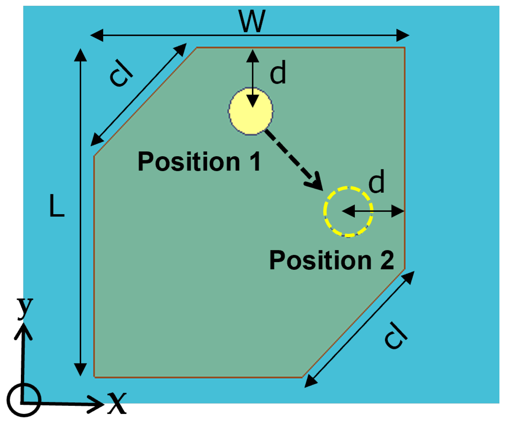
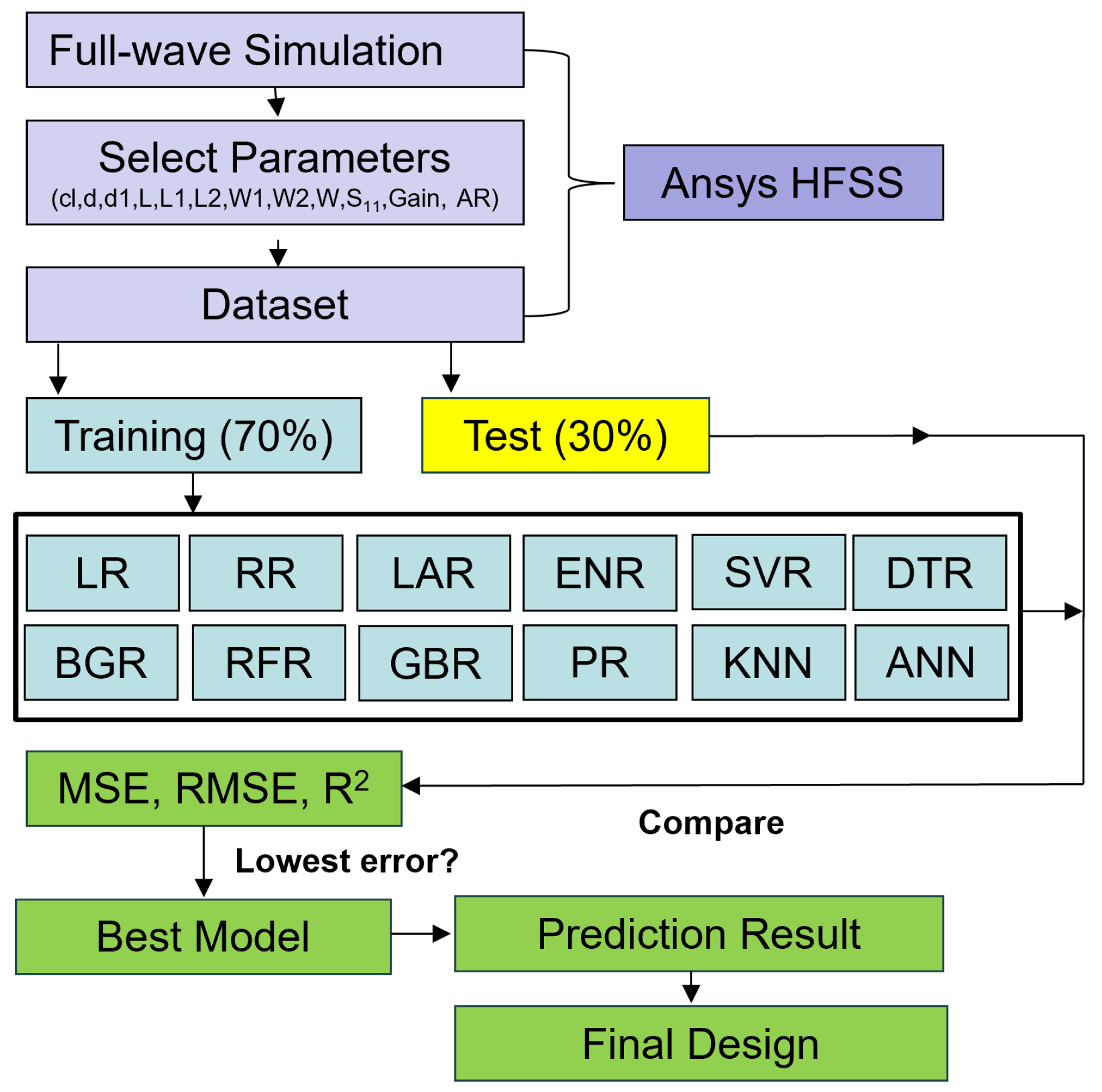
2. Antenna Design Using Machine Learning Approach

Figure 1 and Figure 2 show the top view and side view of the patch antenna with its different features ( c l , d, L, and W), respectively. The substrate is RT/Duroid 5880 ( ϵ r = 2.2 and tan δ = 0.009), with a thickness of 0.79 mm. The antenna shows two possible orthogonal feeds: Position 1 and Position 2. Each position is used to realize either left-hand circular polarization (LHCP) or right-hand circular polarization (RHCP). The antenna is not aimed at serving the purpose of dual polarization (LHCP and RHCP). Hence, LHCP and RHCP will not be obtained simultaneously. The antenna is a square corner-truncated patch. We anticipate that both LHCP and RHCP can be obtained for the same L, W, and cl values by feeding the antenna at a distance ‘d’ away from the edge of the antenna at Position 1 and Position 2 in an alternating manner. Therefore, considering the same value of ‘d,’ we can use ML algorithms to predict the LHCP and RHCP antenna design parameters.

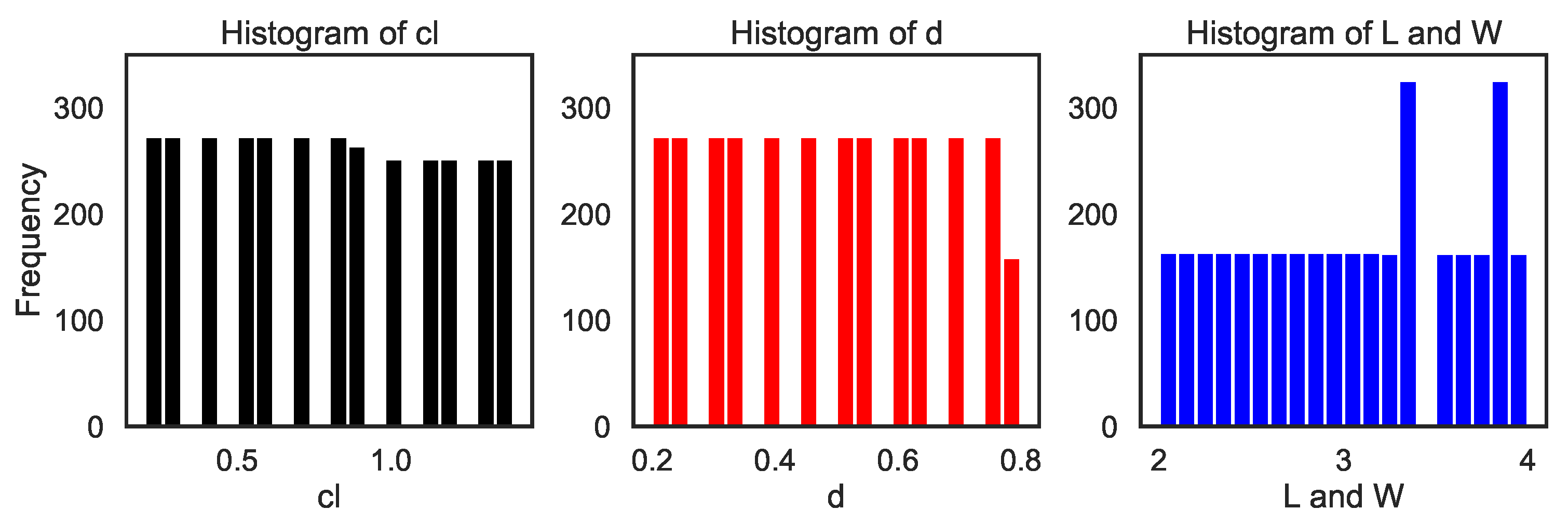
2.1. Data Generation and Model Building

The complete framework to find an effective ML model is shown in Figure 3. The full-wave simulation was used to generate 715 arbitrary datasets of four features ( c l , d, L, and W) and three corresponding targets ( | S 11 | , gain, and AR) at 32 GHz. To generate the dataset, we conducted a parametric analysis using the High-Frequency Structure Simulator (HFSS). The initial values of cl, dl, L, and W ranged from 0.1 mm, 0.2 mm, 2 mm, and 2 mm, respectively, with increments of 0.1 mm. The final values reached 1.8 mm, 0.8 mm, 4 mm, and 4 mm, respectively. Since we employed a square-shaped microstrip patch antenna, the values of L and W were kept similar. The data distribution is visually represented in the histogram plot shown in Figure 4. The datasets are then trained using 12 different ML regression models based on linear regression (LR), ridge regression (RR), lasso regression (LAR), elastic net regression (ENR), decision tree regression (DTR), bagging regression (BGR), random forest regression (RFR), gradient boosting regression (GBR), polynomial regression (PR), SVR, KNN, and ANN.

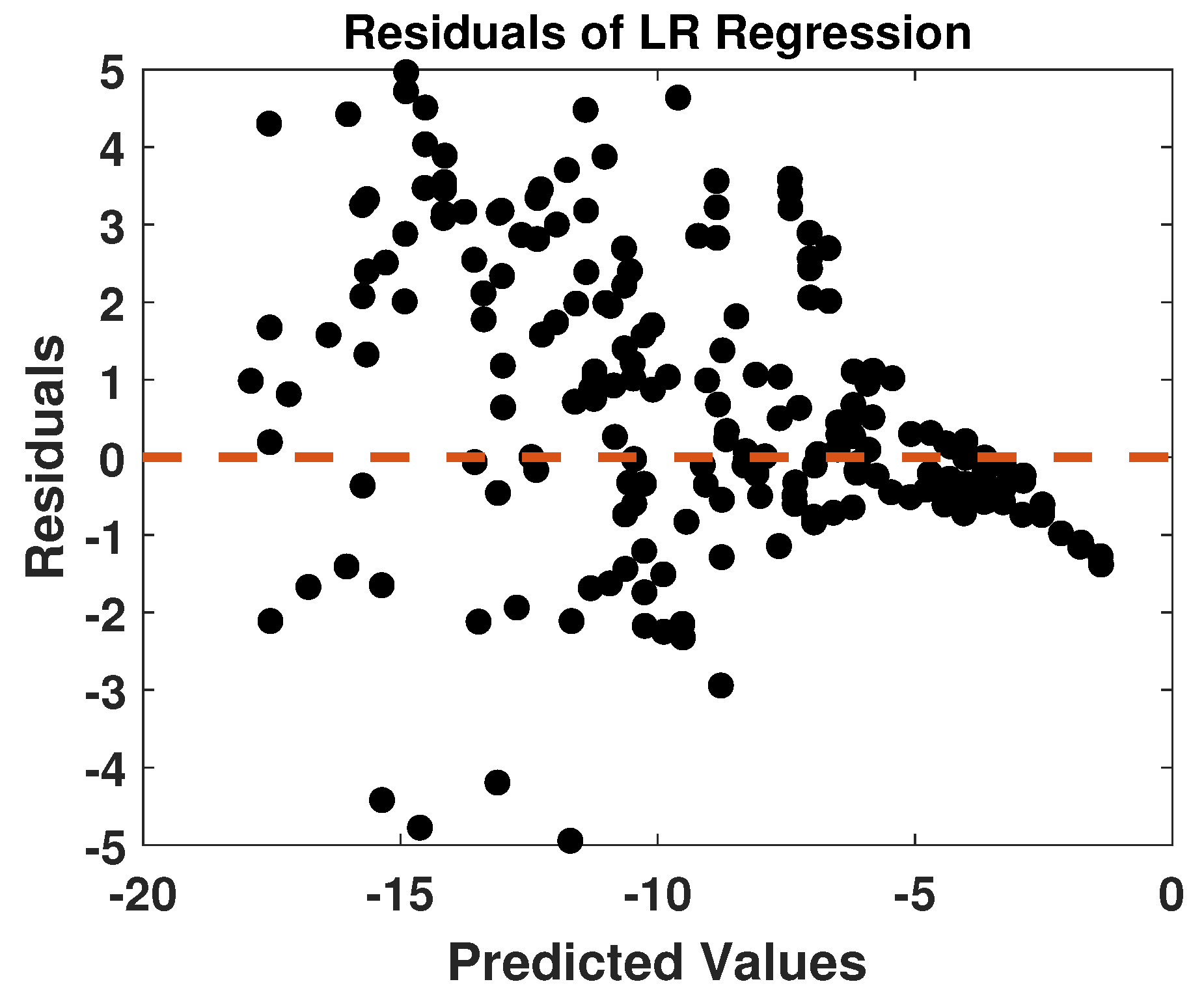
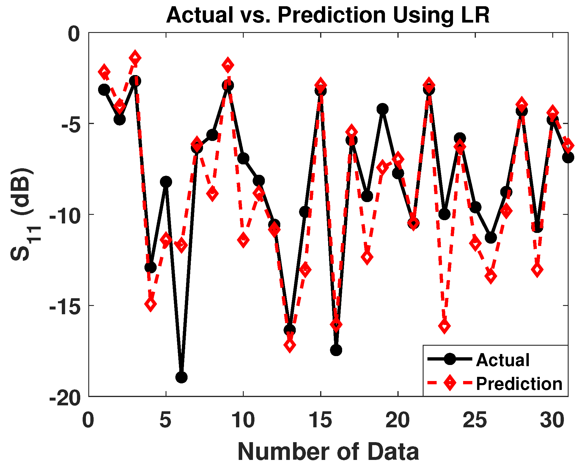
2.1.1. Linear Regression

The LR is one of the most straightforward techniques in statistics and ML. LR results in a linearly separable relation between the dependent (targets) and independent (features) variables from the observed antenna dataset. This approach minimizes the cost function during the fitting phase, resulting in quick calculations for predicting antenna parameters [14].

2.1.2. Ridge Regression

The RR uses a regularization method (L2 regularization) to estimate the magnitude of the coefficient of multiple regression models when independent antenna variables (features) are highly correlated. This technique lowers the standard errors by introducing some bias into the usual linear regression for antenna parameter prediction [15].

2.1.3. Lasso Regression

The LAR uses a regularization (L1 regularization) that employs the shrinkage method to optimize the cost function in the event that there are many antenna features [16].

2.1.4. Elastic Net Regression

The L1 and L2 penalties of the lasso and ridge methods are linearly combined in the regularized regression technique, known as the elastic net [17].

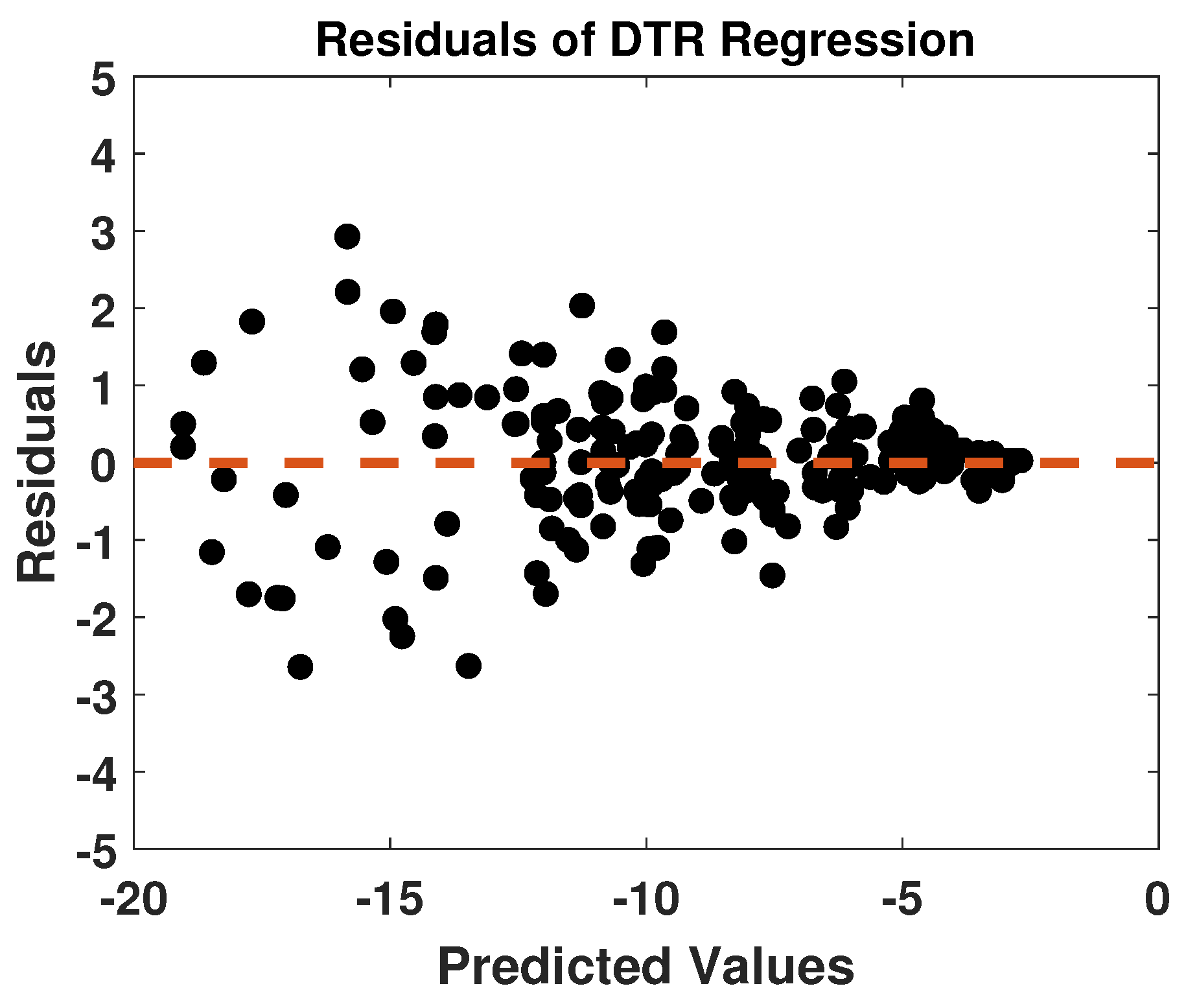
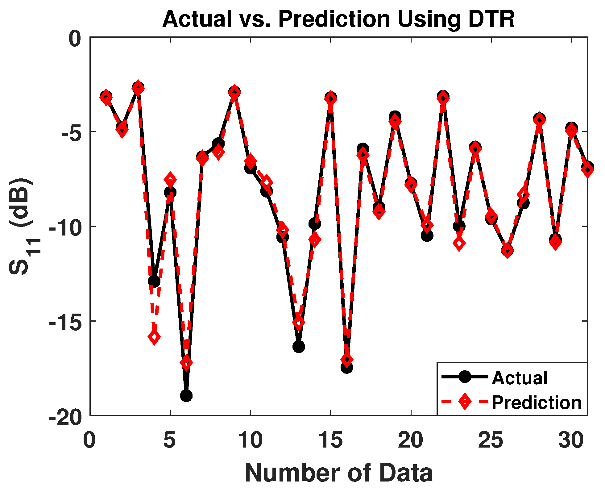
2.1.5. Decision Tree Regression

The DTR is a widely used method for its practicality and efficiency. A decision tree uses a tree-like structure to generate regression models. It incrementally develops an associated decision tree while segmenting the antenna dataset into smaller sections [18].

2.1.6. Bagging Regression

The BGR is an ensemble meta-estimator that fits base regressors one at a time to random subsets of the original dataset. Then, it combines each prediction into a single final prediction. When employed with decision trees, BGR dramatically increases the stability of models by enhancing accuracy and lowering variance, which removes the over-fitting concern of antenna parameters [19].

2.1.7. Random Forest Regression

The RFR is a supervised learning technique that leverages the ensemble learning approach for regression. The ensemble learning method combines predictions from various ML algorithms to provide predictions of different antenna parameters [20].

2.1.8. Gradient Boosting Regression

The GBR is a widely adopted ML technique for predictive modeling, particularly in regression problems. It is a family of ensemble methods that combines many models trained to make antenna parameter predictions. The operational mechanism of GBR involves the iterative addition of weak decision trees to the ensemble, each trained to address the errors generated by the previous model in the sequence [21].

2.1.9. Support Vector Regression

The SVR is a popular ML method representing a variation of the SVM approach. The SVR technique can be employed to address both classification and regression problems. Regarding antenna parameter prediction, SVR endeavors to identify a function that minimizes margin violations while simultaneously fitting the training data [22].

2.1.10. Polynomial Regression

The connection between independent variables (antenna characteristics) and dependent variables (antenna objectives) can be represented as an nth-degree polynomial. During the training of regression models, the fitting curve can be identified. PR is particularly well-suited for antennas that exhibit highly nonlinear behavior [23]. In our case, we employ an 8th-order PR.

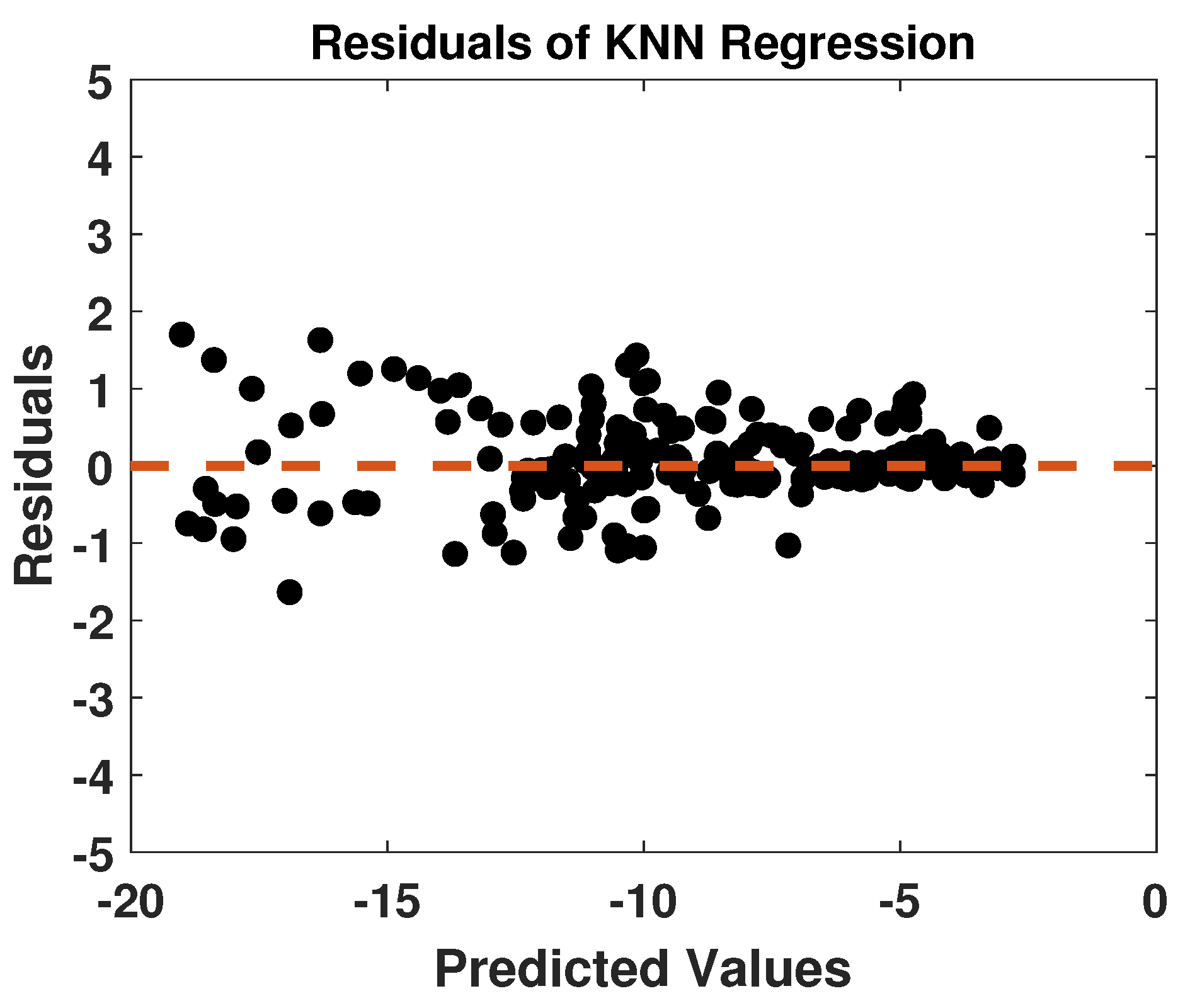
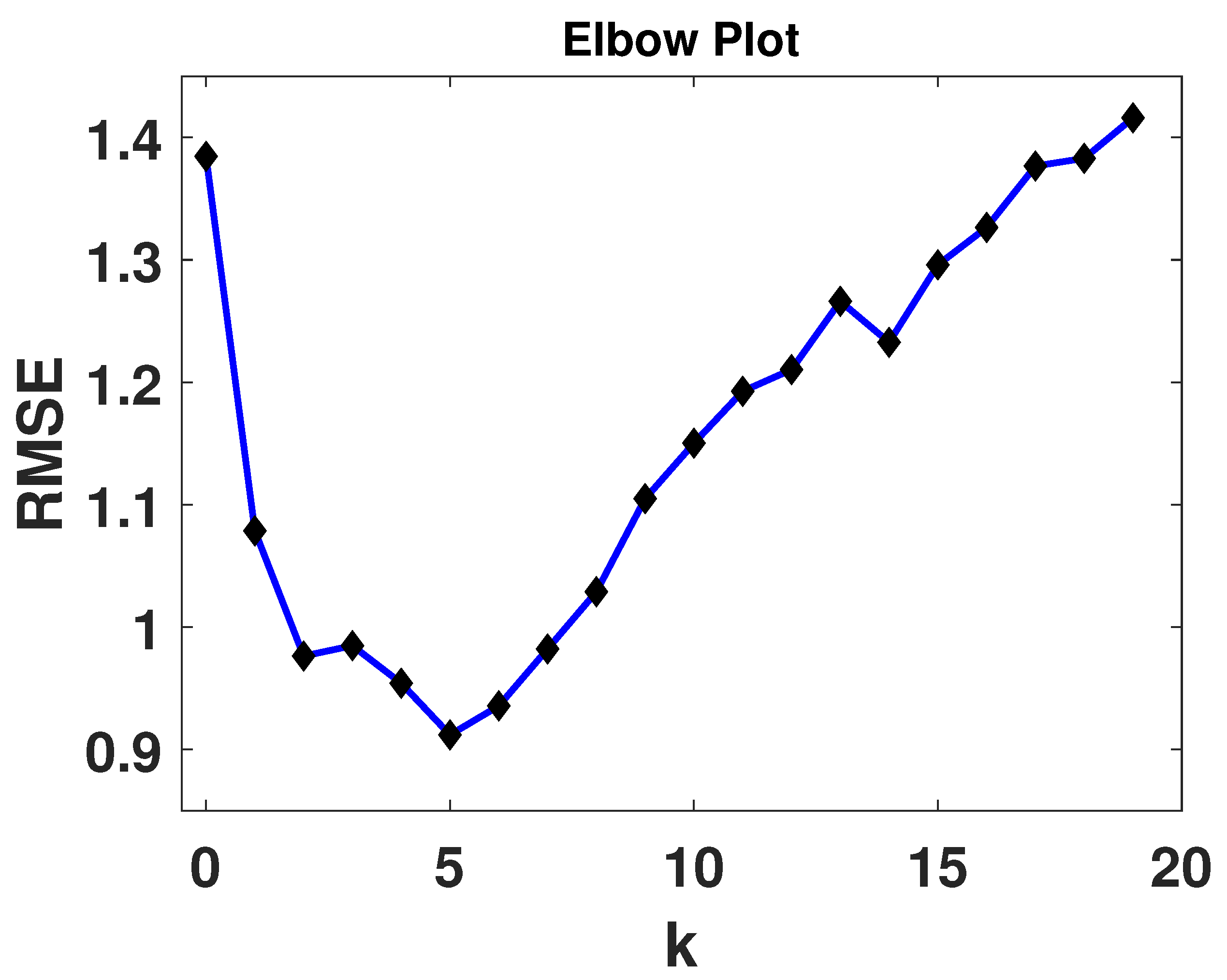
2.1.11. K-Nearest Neighbor Regression

The KNN is a straightforward ML algorithm applied for classification and regression. KNN saves all of the available data, and new input is categorized based on how similar it is to the already recorded data. Typically, a distance metric, such as the Manhattan distance or Euclidean distance, is used to construct the similarity measure. A hyperparameter that needs to be set beforehand is the value of k. A proper way to find the value of k using the elbow method is shown in Figure 5. It is a representation of k vs. error (RMSE). The value of RMSE is lowest for k = 5 , and that was determined using grid search cross-validation (GridsearchCV). KNN provides the new data point of the antenna during regression, which shows the average value of the k nearest neighbors [13].

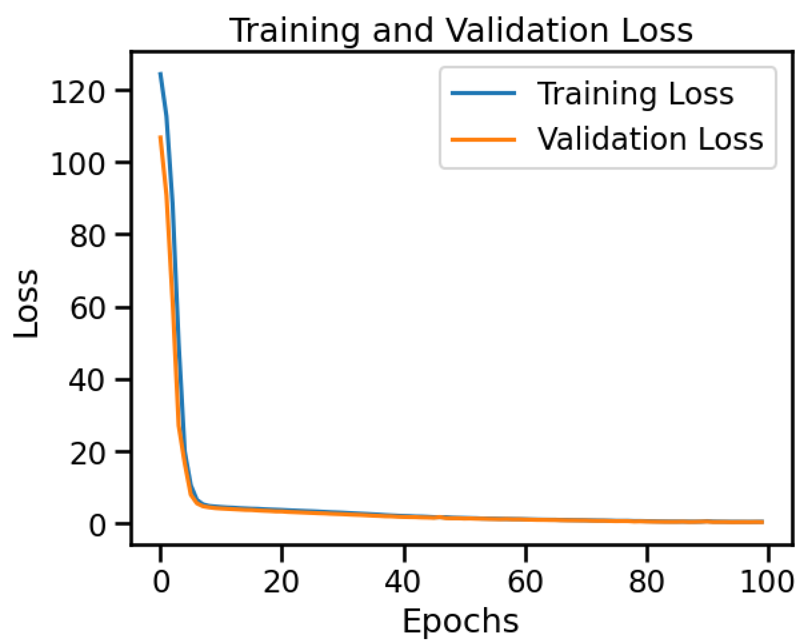
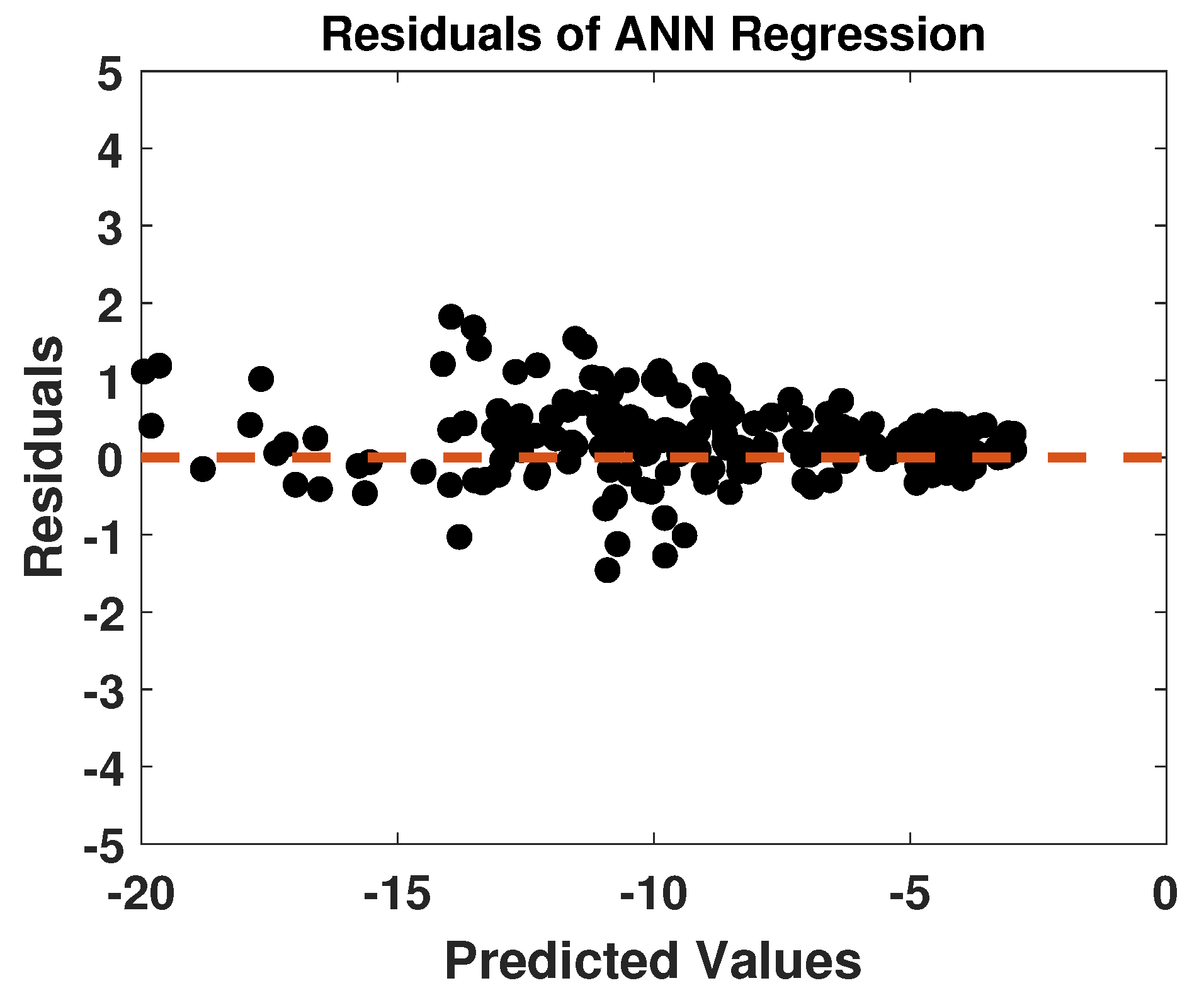
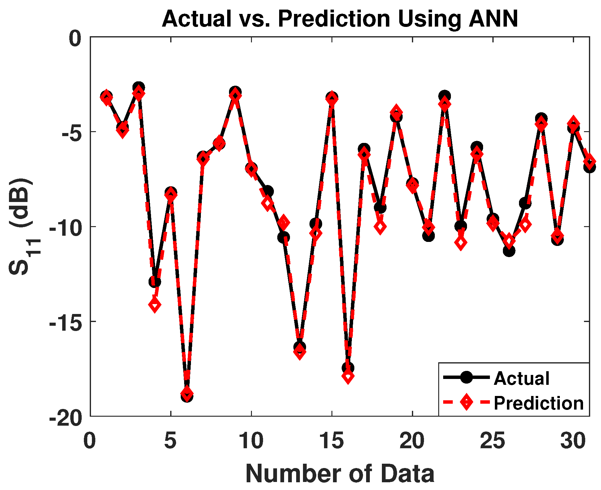
2.1.12. Artificial Neural Network Regression

ANN regression proves highly effective when dealing with highly non-linear datasets. Including activation functions within each hidden layer of an ANN facilitates its capacity to comprehend intricate non-linear associations between input features and the target variable. This capability enables ANNs to make highly accurate predictions, particularly when complex, non-linear relationships exist in the data [4]. Our study employs a network architecture comprising five hidden layers to explore and leverage these capabilities. We initially started with fewer hidden layers for ANN regression. However, we discovered highly non-linear connections between the input features and the target variable. As a result, the model’s capacity to approximate those relationships was improved by adding more hidden layers (five). Figure 6 shows the epochs vs. loss for ANN regression.
The precision of all the above-mentioned ML algorithms depends on the antenna dataset. Therefore, finding an efficient ML model to predict antenna parameters is necessary. The complete framework to find an effective ML model is shown in Figure 3. The datasets are split into two categories, where 70% of the data is used to train the model, and 30% is used for testing. We used Scikit-learn extensively for different regressions, error metrics, hyperparameter tuning, and cross-validation throughout our study. The model validation using different error metrics is described in the following section.

2.2. Model Validation and Antenna Prediction

The performance of each model is analyzed by computing and comparing the MAE, MSE, RMSE, and R 2 score to find the best model using the Python programming language on Jupyter Notebook. The lowest MAE, MSE, and RMSE and the highest R 2 score are desirable for accurate prediction. Notably, the ANN model exhibits the lowest MAE, MSE, and RMSE and the highest R 2 score. Table 1 shows the error metrics for all regression models. The second model, which shows better results, is KNN. Figure 7 shows the bar chart indicating MAE, MSE, RMSE, and R 2 scores for all regression models used in this paper. Figure 8, Figure 9, Figure 10 and Figure 11 show the residual | S 11 | results for LR, DTR, KNN, and ANN regression, respectively. Figure 12, Figure 13, Figure 14 and Figure 15 show the actual and predicted | S 11 | results for LR, DTR, KNN, and ANN regression, respectively.
The ANN regression shows a more accurate prediction compared to LR and DTR. For instance, in the LR model, the large number of residuals is responsible for the highest MAE, MSE, and RMSE and the lowest R 2 scores, as shown in Table 1. We note that the KNN can be a secondary option, as it shows results close to ANN. However, PR, BGR, GBR, RFR, and DTR models can also be used as secondary selections with comparatively lower MAE, MSE, and RMSE, among other models (LR, RR, LAR, ENR, and SVR). Table 2 shows the predicted | S 11 | , realized gain, and AR for an arbitrary antenna ( c l = 0.88 mm, d = 0.58 mm, L, and W = 2.73 mm) at 32 GHz, with values of −13.70 dB, 7.63 dBic, and 0.71 dB, respectively. The features or design variables are chosen arbitrarily, as our model can predict design targets of a circular polarized (CP) antenna for any given dataset.
Designing a circular polarized CTMPA is more complex than designing a linearly polarized square patch antenna, as the design parameters ( | S 11 | , gain, and AR) can vary significantly with changes in feeding point (d), corner length ( c l ), and antenna dimensions (L and W). The conventional full-wave simulation is used to optimize the CP antenna’s gain, return loss, and AR. However, this is time-consuming and often exhausts resources. Our approach offers a way to predict the design parameters of CTMPA before conducting actual simulations, making it much faster and more efficient. To the best of our knowledge, we are the first to introduce different ML algorithms for predicting the design parameters of a CTMPA antenna.

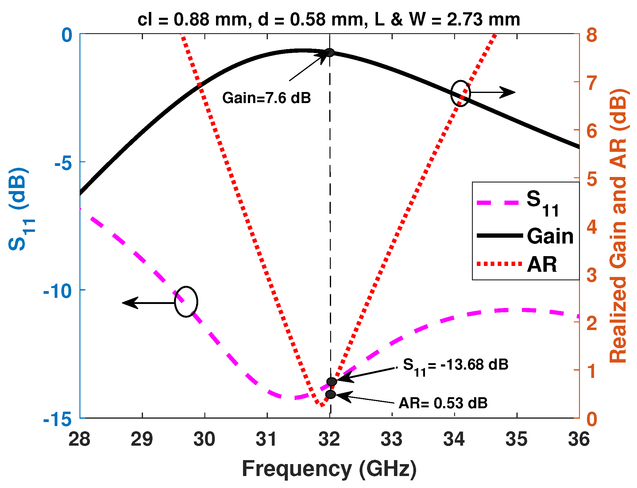
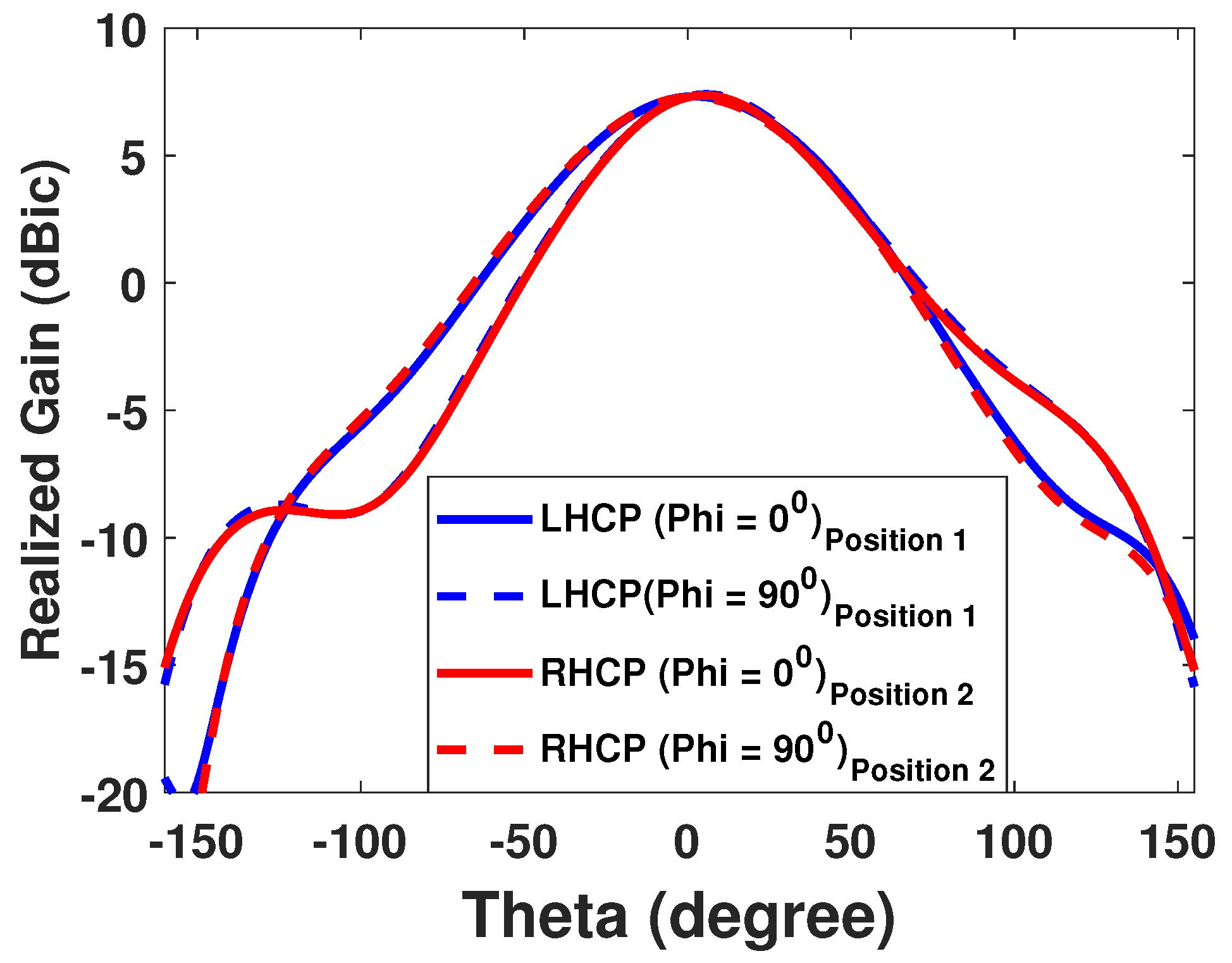
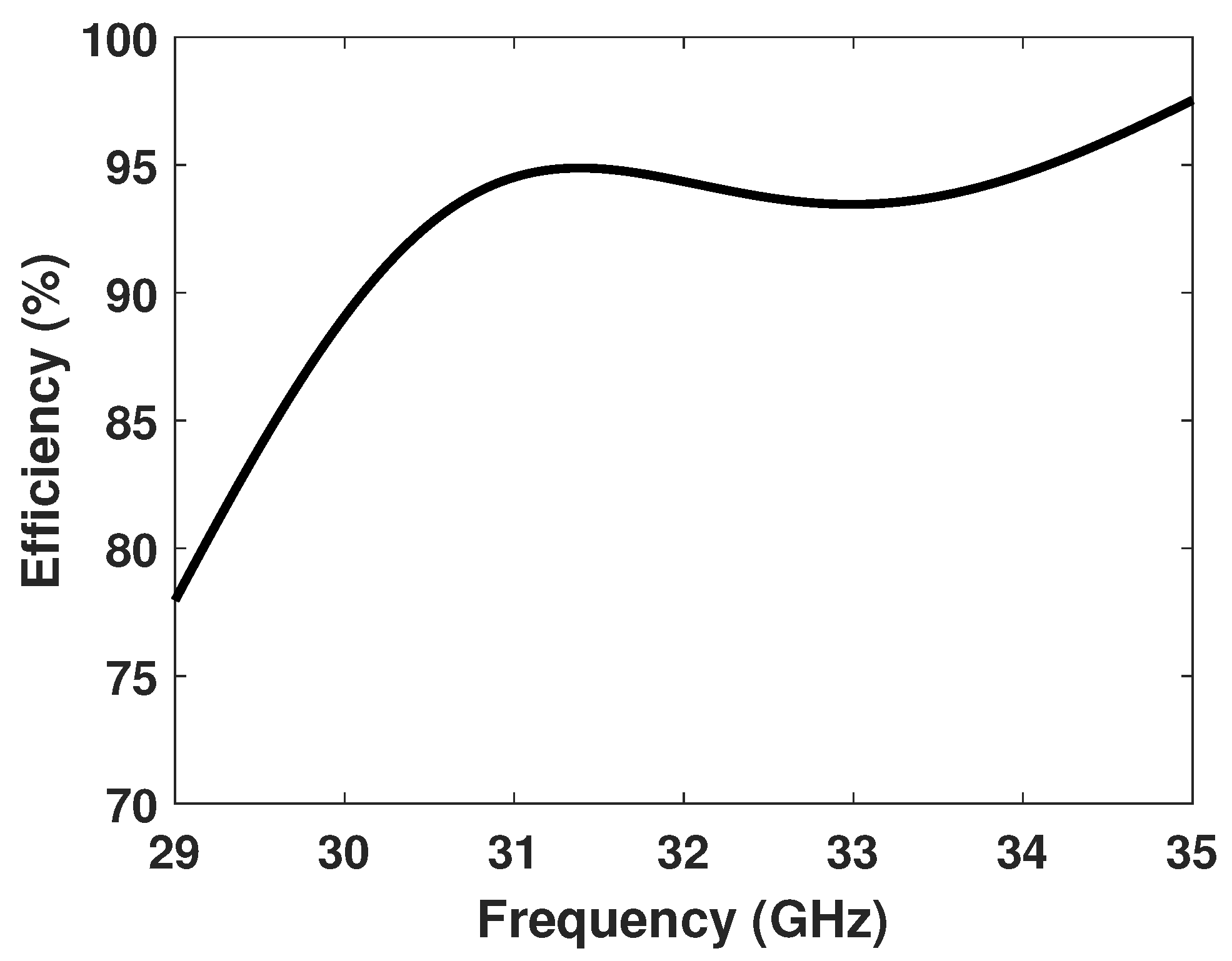
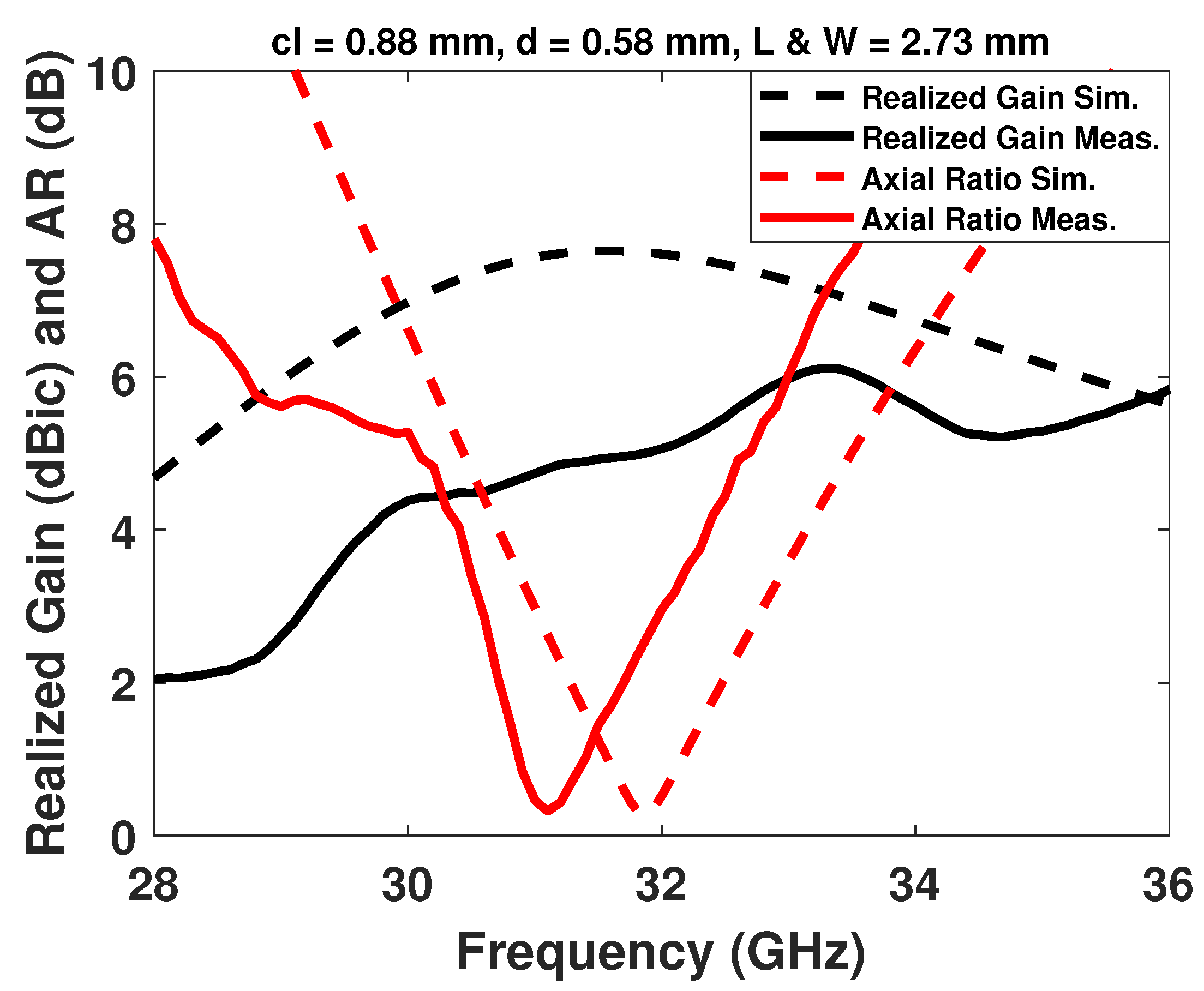
2.3. Antenna Design Validation Using Full-Wave Simulation

We validated the predicted antenna ( c l = 0.88 mm, d = 0.58 mm, L, and W = 2.73 mm) using full-wave simulation (High-Frequency Structure Simulator (HFSS)). The target prediction using all ML algorithms and true values (full-wave simulation) is shown in Table 2. As expected, the simulated | S 11 | , realized gain, and AR are almost identical to the ANN prediction at 32 GHz, with values of −13.68 dB, 7.6 dBic, and 0.53 dB, respectively, as shown in Figure 16. Our objectives are to obtain a gain of >5 dBic across a 10% bandwidth, an axial ratio (AR) of <3 dB, and a return loss of <−10 dB. Meanwhile, we obtained a gain of >6.4 dBic across a 14% bandwidth (29.5 GHz–34 GHz) and an axial ratio (AR) of <3 dB (31 GHz–33 GHz).
We validated the LHCP and RHCP using the same antenna parameters by switching the orthogonal feeding position from Position 1 to Position 2, as illustrated in Figure 1. Our presented antenna is a square patch with corner perturbation, providing LHCP and RHCP alternatively using two orthogonal feedings. Our ML model accurately predicts the design of both individual LHCP and RHCP antennas. Figure 17 shows the realized gain and AR at 32 GHz for both LHCP and RHCP when the feeding position is in Position 1 and Position 2, respectively. The broadside realized gain is 7.6 dBic at 32 GHz in the elevation plane for both polarizations. Additionally, the simulated AR at the broadside is 0.53 dB. As such, the simulated result greatly agrees with the prediction result. This verification demonstrates that the ANN model outperforms all other ML regression models in terms of prediction.
ANN regression can be used where a non-linear relationship among the data frame is dominant. Due to the presence of an activation function in each hidden layer, ANN can learn the non-linear complex relationship between the features and target and can predict results accurately. In contrast, KNN stores all available data and categorizes new input based on its similarity to the recorded data using a distance metric, such as the Manhattan or Euclidean distance. However, in other models, all the data are not saved. For instance, linear regression predicts a linear relationship between dependent and independent variables and identifies the optimal fitting line/curve for efficient prediction. In such cases, the best result is obtained when the variables have a linear relationship with each other. However, our dataset does not exhibit a linear relationship among all variables. Instead, datasets are random. Therefore, ANN and KNN would be ideal models for our prediction. Additionally, bagging regression, random forest regression, gradient boosting regression, and decision tree regression can be used as secondary options for prediction, as these ML techniques use small, tree-like structures for training and prediction. Figure 18 shows the antenna’s efficiency for both polarizations, and 94% efficiency was achieved at 32 GHz.

2.4. Antenna Prediction Time

The simulation was done on a 2.9 GHz processor with 80 GB of RAM installed. The maximum time to complete the sweep in a single frequency (32 GHz) is about 63,000 ms. In contrast, the target prediction time for the ML algorithm is only a few milliseconds using the same operating system, as shown in Table 3. Indeed, the prediction time decreases several orders of magnitude (∼10 4 ) using the ML approach compared to conventional full-wave simulation.

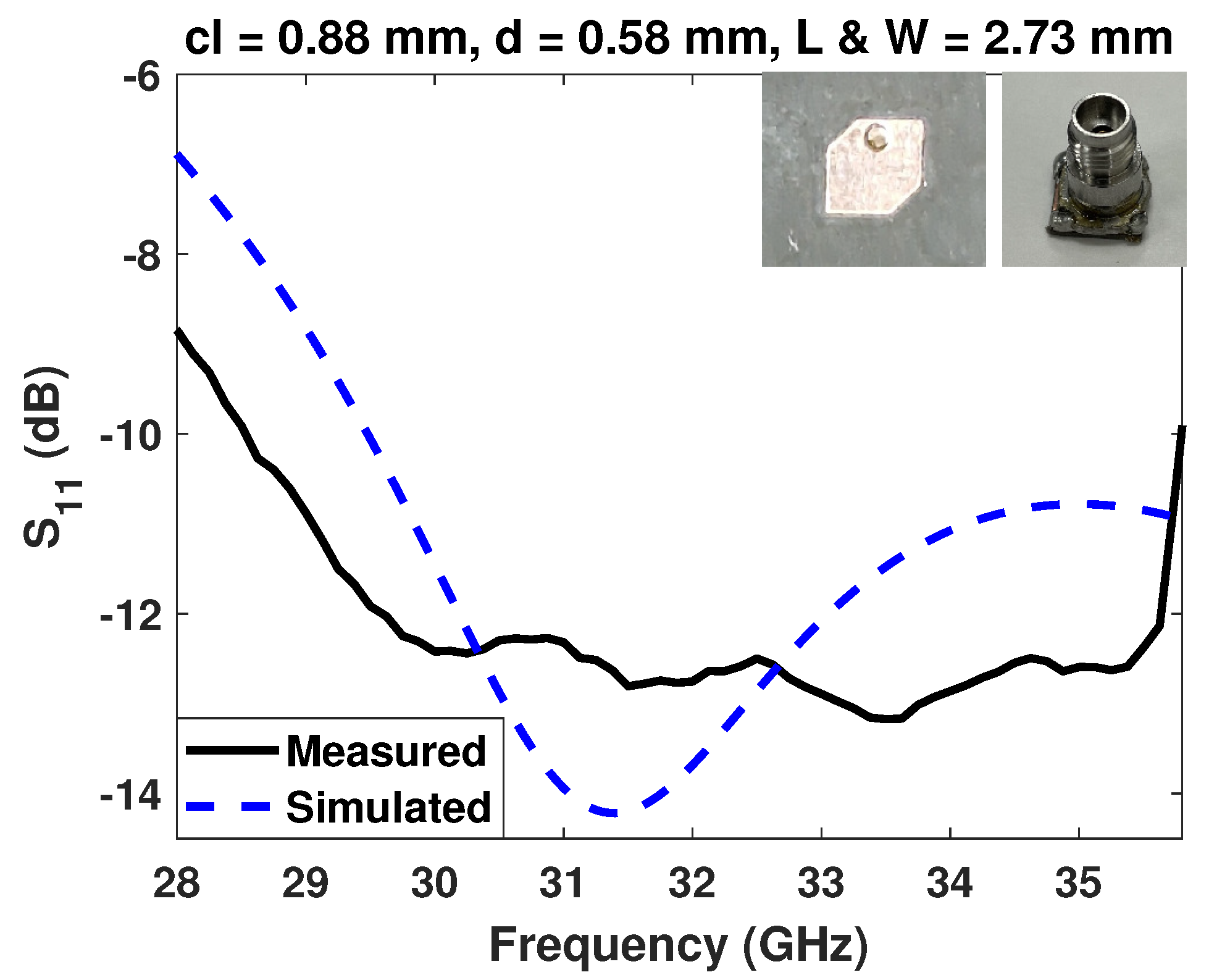
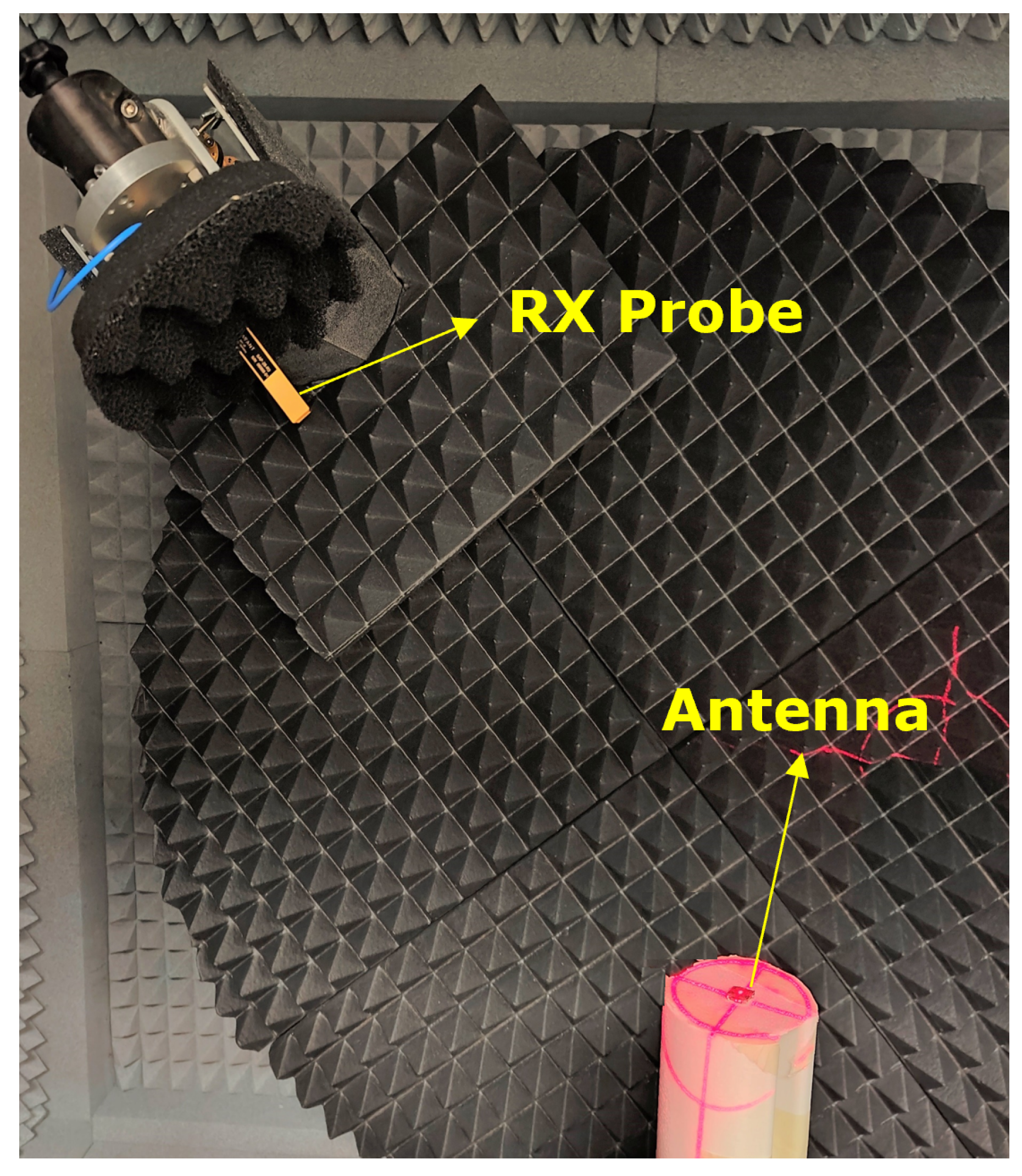
3. Fabrication and Measurement

We fabricated a prototype for the LHCP to validate the concept. A standard milling machine was used for the fabrication. A 2.4 mm connector was used to feed the antenna for measurement. Figure 19 shows the simulated and measured | S 11 | of the LHCP antenna. The predicted | S 11 | is −13.7 dB, the simulated | S 11 | is −13.68 dB, and the measured | S 11 | is −12.75 dB at 32 GHz. Therefore, the measured data agree well with the simulated and predicted values. Figure 20 shows the pattern measurement setup at the Ka-band (26.5 GHz–40 GHz). Figure 21 shows the measured realized gain of the LHCP antenna for both the E plane and the H plane at 32 GHz. The maximum gain at 32 GHz is 5.01 dBic, and the 3 dB beam width is 68 0 , whereas the simulated beam width is 58 0 . Figure 22 shows the simulated and measured realized gain and AR of the LHCP antenna. The predicted, simulated, and measured realized gains are 7.63 dBic, 7.6 dBic, and 5.01 dBic, respectively, at 32 GHz. The predicted, simulated, and measured AR are 0.71 dB, 0.53 dB, and 2.3 dB at 32 GHz. The slight discrepancy between the simulation and fabrication outcomes is due to fabrication inaccuracy and soldering of the connector. During the soldering process, we encountered a challenge where the antenna’s ground plane did not securely attach to the connector base. To address this issue within the constraints of our fabrication process, we applied additional soldering resin to establish a connection. We believe this irregularity in the ground plane’s current distribution contributed to discrepancies between the simulated and measured data. Under ideal conditions, we would expect these discrepancies to be significantly reduced. However, the result is acceptable for validating the proof of concept. The properties of the different ML algorithms for designing the antenna are summarized in Table 4. Our study introduces an approach that considers multiple objectives, including | S 11 | , AR, and gain, as well as antenna polarization. This contrasts with most other research efforts, where the primary focus is estimating | S 11 | .

4. Conclusions

This paper presents an efficient and intelligent ML approach to predict the | S 11 | , gain, and AR of a circularly polarized microstrip antenna. The goal is to achieve full polarization diversity with a wide 3 dB axial ratio (30.9 GHz–32.8 GHz) and a stable gain of >5 dBic. Twelve different ML regression models were evaluated using four error metrics (MAE, MSE, RMSE, and R 2 score). Among them, the ANN model performed best. A model was then predicted and validated using full-wave simulation. Also, a prototype was fabricated and measured. The predicted, simulated, and measured results agreed well, indicating that this approach can save significant computational resources and time in designing an efficient circular polarized antenna for CubeSat downlink applications.

Author Contributions

E.A.A. and M.N.U. contributed on the conceptualization and methodology of this work. M.N.U. and M.O. worked on machine learning validation in Python. M.K.I. conducted an investigation and measurements. All authors contributed to writing the paper. E.A.A. supervised the overall activities of the project. All authors have read and agreed to the published version of the manuscript.

Funding

This work was supported in part by the National Science Foundation, USA grant 2030250 and by the U.S. Air Force Office of Scientific Research grant FA9550-18-1-0191.

Data Availability Statement

Not applicable.

Conflicts of Interest

The authors declare no conflict of interest.

References

  1. Uddin, M.N.; Choi, S. Non-uniformly powered and spaced corporate feeding power divider for high-gain beam with low SLL in millimeter-wave antenna array. Sensors 2020, 20, 4753. [Google Scholar] [CrossRef] [PubMed]
  2. Chahat, N.; Decrossas, E.; Gonzalez, D.; Yurduseven, O.; Radway, M.; Hodges, R.; Estabrook, P.; Baker, J.; Cwik, T.; Chattopadhyay, G. A review of CubeSat antennas: From low Earth orbit to deep space. IEEE Antennas Propag. Mag. 2019, 61, 37–46. [Google Scholar] [CrossRef]
  3. Uddin, M.N.; Tarek, M.N.A.; Islam, M.K.; Alwan, E.A. A Reconfigurable Beamsteering Antenna Array at 28 GHz Using a Corporate-fed 3-Bit Phase Shifter. IEEE Open J. Antennas Propag. 2023, 4, 126–140. [Google Scholar] [CrossRef]
  4. Sharma, Y.; Zhang, H.H.; Xin, H. Machine learning techniques for optimizing design of double T-shaped monopole antenna. IEEE Trans. Antennas Propag. 2020, 68, 5658–5663. [Google Scholar] [CrossRef]
  5. Chen, W.; Wu, Q.; Yu, C.; Wang, H.; Hong, W. Multibranch Machine Learning-Assisted Optimization and Its Application to Antenna Design. IEEE Trans. Antennas Propag. 2022, 70, 4985–4996. [Google Scholar] [CrossRef]
  6. Jae Hee, K.; Sang Won, C. A deep learning-based approach for radiation pattern synthesis of an array antenna. IEEE Access 2020, 8, 226059–226063. [Google Scholar]
  7. Christodoulou, C.G.; Rohwer, J.A.; Abdallah, C.T. The use of machine learning in smart antennas. In Proceedings of the 2004 IEEE Antennas and Propagation Society Symposium, Monterey, CA, USA, 20 May 2004; pp. 321–324. [Google Scholar]
  8. Pastorino, M.; Randazzo, A. A smart antenna system for direction of arrival estimation based on a support vector regression. IEEE Trans. Antennas Propag. 2005, 54, 2161–2168. [Google Scholar] [CrossRef]
  9. Pastorino, M.; Randazzo, A. The SVM-Based Smart Antenna for Estimation of the Directions of Arrival of Electromagnetic Waves. IEEE Trans. Antennas Propag. 2006, 55, 1918–1925. [Google Scholar] [CrossRef]
  10. Joung, J. Machine Learning-Based Antenna Selection in Wireless Communications. IEEE Communications Letters 2016, 20, 2241–2244. [Google Scholar] [CrossRef]
  11. Hilal, M.E.M.; Tarek, N.; Salwa, K.A.K. A review on the design and optimization of antennas using machine learning algorithms and techniques. Int. J. RF Microw. Comput.-Aided Eng. 2020, 30, e22356. [Google Scholar]
  12. Murphy, K.P. Machine Learning: A Probabilistic Perspective (Adaptive Computation and Machine Learning Series); The MIT Press: London, UK, 2018. [Google Scholar]
  13. Cui, L.; Zhang, Y.; Zhang, R.; Liu, Q.H. A Modified Efficient KNN Method for Antenna Optimization and Design. IEEE Trans. Antennas Propag. 2020, 68, 6858–6866. [Google Scholar] [CrossRef]
  14. Shi, D.; Lian, C.; Cui, K.; Chen, Y.; Liu, X. A Modified An Intelligent Antenna Synthesis Method Based on Machine Learning. IEEE Trans. Antennas Propag. 2022, 70, 4965–4976. [Google Scholar] [CrossRef]
  15. Runze, H.; Vikass, M.; Ryutaro, H.; Hideo, Y.; Fumie, C. A Statistical Parsimony Method for Uncertainty Quantification of FDTD Computation Based on the PCA and Ridge Regression. IEEE Trans. Antennas Propag. 2019, 67, 4726–4737. [Google Scholar]
  16. Tasfia, N.; Hasan, M.N. Artificial Magnetic Conductor Unit Cell Design Using Machine Learning Algorithms. In Proceedings of the 2022 IEEE International IOT, Electronics and Mechatronics Conference (IEMTRONICS), Toronto, ON, Canada, 4 June 2022; pp. 1–7. [Google Scholar]
  17. Chris, H. Elastic net regression modeling with the orthant normal prior. J. Am. Stat. Assoc. 2011, 106, 1383–1393. [Google Scholar]
  18. Shilpa, V.P.; Santhosh, K.S.S.; Asha, J. Designing of a 5G Multiband Antenna Using Decision Tree and Random Forest Regression Models. In Proceedings of the 2021 8th International Conference on Signal Processing and Integrated Networks (SPIN), Delhi, India, 27 August 2022; pp. 626–631. [Google Scholar]
  19. Breiman, L. Bagging predictors. Mach. Learn. 1996, 24, 123–140. [Google Scholar] [CrossRef]
  20. Nazmia, K.; Dianing, N.N.P.; Yuli, K.N. Random Forest Regression for Predicting Metamaterial Antenna Parameters. In Proceedings of the 2020 2nd International Conference on Industrial Electrical and Electronics (ICIEE), Lombok, Indonesia, 21 October 2020; pp. 174–178. [Google Scholar]
  21. Hakan, K.; Umut, E.A.; Peyman, M. Ensemble-based surrogate modeling of microwave antennas using XGBoost algorithm. Int. J. Numer. Model. Electron. Netw. Devices Fields 2022, 35, e2950. [Google Scholar]
  22. Xi, W.D.; MI, D.L.; Hao, W.T.; Yu, H.Z. Design of Compact Patch Antenna Based on Support Vector Regression. Radioengineering 2022, 31, 339–345. [Google Scholar]
  23. Easum, J.A.; Nagar, J.; Werner, P.L.; Werner, D.H. Efficient Multiobjective Antenna Optimization with Tolerance Analysis Through the Use of Surrogate Models. IEEE Trans. Antennas Propag. 2018, 66, 6706–6715. [Google Scholar] [CrossRef]
  24. Chen, Y.; Elsherbeni, A.Z.; Demir, V. Machine Learning for Microstrip Patch Antenna Design: Observations and Recommendations. In Proceedings of the 2022 United States National Committee of URSI National Radio Science Meeting (USNC-URSI NRSM), Boulder, CO, USA, 4 January 2022; pp. 256–257. [Google Scholar]
  25. Haque, M.A.; Sarker, N.; Sawaran Singh, N.S.; Rahman, M.A.; Hasan, M.N.; Islam, M.; Zakariya, M.A.; Paul, L.C.; Sharker, A.H.; Abro, G.E.M.; et al. Dual Band Antenna Design and Prediction of Resonance Frequency Using Machine Learning Approaches. Appl. Sci. 2022, 12, 10505. [Google Scholar] [CrossRef]
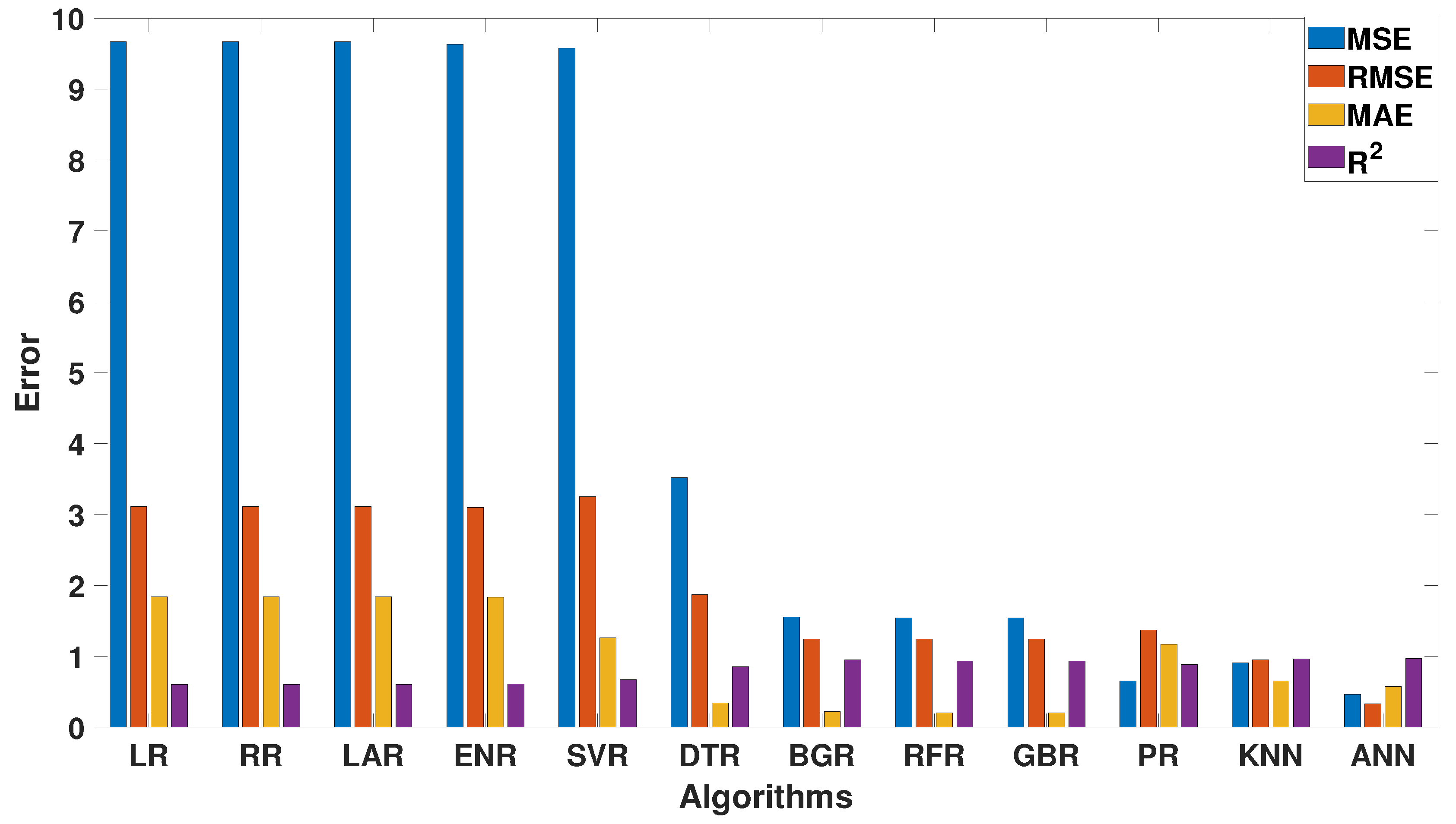
Figure 1. Top view of the patch antenna operating at 32 GHz (two feeding positions suggest that, by using the same value of ‘d’, LHCP and RHCP can be obtained).
Electronics 12 04195 g001
Figure 2. Stack-up side view.
Electronics 12 04195 g002
Figure 3. Framework of the antenna design using ML algorithms.
Electronics 12 04195 g003
Figure 4. Histograms of the dataset of features (cl, d, L, and W) used for the ML algorithms.
Electronics 12 04195 g004
Figure 5. Elbow plot showing the k vs. RMSE.
Electronics 12 04195 g005
Figure 6. Epochs vs. loss plot of ANN regression.
Electronics 12 04195 g006
Figure 7. Bar chart showing the error for different ML regression models shown in Table 1.
Electronics 12 04195 g007
Figure 8. Plot showing the residuals of | S 11 | using linear regression (LR).
Electronics 12 04195 g008
Figure 9. Plot showing the residuals of | S 11 | using decision tree regression (DTR).
Electronics 12 04195 g009
Figure 10. Plot showing the residuals of | S 11 | using KNN regression.
Electronics 12 04195 g010
Figure 11. Plot showing the residuals of | S 11 | using ANN regression.
Electronics 12 04195 g011
Figure 12. Plot showing the actual vs. predicted | S 11 | using LR.
Electronics 12 04195 g012
Figure 13. Plot showing the actual vs. predicted | S 11 | using DTR.
Electronics 12 04195 g013
Figure 14. Plot showing the actual vs. predicted | S 11 | using KNN regression.
Electronics 12 04195 g014
Figure 15. Plot showing the actual vs. predicted | S 11 | using ANN regression.
Electronics 12 04195 g015
Figure 16. Full-wave simulation showing | S 11 | , realized gain, and AR of predicted antenna.
Electronics 12 04195 g016
Figure 17. Full-wave simulation showing realized gain for both planes (E and H) for two different feeding positions at 32 GHz.
Electronics 12 04195 g017
Figure 18. Simulated efficiency of antenna.
Electronics 12 04195 g018
Figure 19. Simulated and measured | S 11 | for the predicted antenna. Inset shows the fabricated antenna top (left) and bottom view with a 2.4 mm connector (right).
Electronics 12 04195 g019
Figure 20. Far-field measurement setup of the fabricated CP antenna operating at 32 GHz.
Electronics 12 04195 g020
Figure 21. Measured realized gain of the predicted antenna for both the E plane and the H plane at 32 GHz.
Electronics 12 04195 g021
Figure 22. Simulated and measured realized gain and AR vs. frequency for the predicted antenna.
Electronics 12 04195 g022
Table 1. Error metrics showing MAE, MSE, RMSE, and R 2 score for different algorithms.
AlgorithmMAEMSERMSER 2
LR1.849.673.110.60
RR1.849.673.110.60
LAR1.849.663.100.60
ENR1.8479.633.100.61
SVR1.269.583.250.67
DTR0.343.521.870.85
BGR0.221.551.240.95
RFR0.201.541.240.93
GBR0.201.541.240.93
PR (8th)0.651.371.170.88
KNN0.110.910.950.96
ANN0.460.330.570.97
Table 2. Predicted | S 11 | , gain, and AR for c l = 0.88 mm, d = 0.58 mm, L, and W = 2.73 mm using different algorithms.
Algorithm | S 11 | (dB)Gain (dBic)AR (dB)
LR−17.436.105.84
RR−17.436.105.84
LAR−17.426.105.86
ENR−17.416.105.86
SVR−15.877.425.63
DTR−14.437.611.16
BGR−14.327.671.21
RFR−14.407.691.16
GBR−13.247.821.65
PR (8th)−13.487.81.57
KNN−13.457.640.82
ANN−13.707.630.71
Full-wave Simulation−13.687.60.53
Table 3. Time comparison for the target ( | S 11 | , gain, and AR) prediction of any random features (viz. L, W, c l and d) at 32 GHz using different methods.
MethodTime (ms)
LR3.67
RR4.78
LAR4.95
ENR3.98
SVR14.9
DTR4.98
BGR41.7
RFR36.9
GBR53.8
PR (8th order)7.6
KNN5.96
ANN4.87
Full-wave Simulation63,000
Table 4. Our work with reported work in the literature.
ReferenceAlgorithmsAntenna TypePolarizationPredicted Objective
[4]Lasso, KNN, and ANNT-monopoleN/A | S 11 |
[13]KNNDipoleN/A | S 11 |
[14]SVMPatch and HornN/A | S 11 |
[24]LRPatchN/A | S 11 |
[25]7 ModelsPatchN/A | S 11 |
Our Work12 ModelsCTMPACircular | S 11 | , AR, and gain
Disclaimer/Publisher’s Note: The statements, opinions and data contained in all publications are solely those of the individual author(s) and contributor(s) and not of MDPI and/or the editor(s). MDPI and/or the editor(s) disclaim responsibility for any injury to people or property resulting from any ideas, methods, instructions or products referred to in the content.

