

OptiDJS+: A Next-Generation Enhanced Dynamic Johnson Sequencing Algorithm for Efficient Resource Scheduling in Distributed Overloading within Cloud Computing Environment


 , , , and
Abstract
:1. Introduction
- Advanced optimization techniques: OptiDJS+ incorporates state-of-the-art optimization techniques to intelligently allocate resources, ensuring an optimal makespan and improved resource utilization.
- Heuristic methods: to adapt to dynamic workloads, OptiDJS+ leverages heuristic methods for on-the-fly decisionmaking, optimizing resource allocation based on real-time demand.
- Adaptive scheduling: in the face of varying workloads, OptiDJS+ dynamically reconfigures resource allocation strategies, maintaining high efficiency and adaptability.
- Real-time monitoring: OptiDJS+ continuously monitors resource usage and workload patterns, enabling timely adjustments to resource allocation and task sequencing.
- Makespanminimization: a primary objective of OptiDJS+ is the minimization of the makespan, thereby optimizing resource usage and ensuring timely task completion.
- Load balancing: OptiDJS+ prioritizes load balancing to distribute tasks evenly across available resources, preventing resource contention and improving system stability.
- Fault tolerance: in the event of resource failures or disruptions, OptiDJS+ employs fault-tolerant strategies to ensure uninterrupted task execution and maintain service reliability.
1.1. Objective of the Study
1.2. Problem Statement
1.3. Major Contributions
- The DHJS method, which aims to maximize both efficiency and cost-effectiveness, is frequently used to optimize difficult engineering project scheduling issues. In this study, we offer a technique for greatly enhancing resource availability in the context of parallel processing in a cloud computing environment.
- The Johnson Bayes design principle, which is essential for rational task sequencing, is adhered to in this study’s proposal of a two-tiered technique to improve work scheduling performance.
- A preset collection of varied virtual machines (VMs) is ultimately created as a result. The provisioning of virtual resources can be sped up by using certain VM settings, especially when tasks are being scheduled. Dynamic task allocation is supported at the secondary level by certain VMs that advise dynamic task-scheduling methods. Comparing their efficacy to current approaches, empirical test findings show that they are more successful at managing resource demands and enhancing cloud scheduling performance. One of the most significant difficulties in the field of cloud computing is task scheduling.
- The second significant benefit is the decrease in resource management expenses for numerous ten ant user infrastructures situated inside a uniformly dispersed data center.
1.4. Paper Organization
2. Related Work
- Approaches for measuring clouds include batch, interactive, and real-time approaches. Batch systems allow the forecasting of throughput and turnaround times. To grade responsiveness and fairness, a live, interactive system that keeps track of deadlines might be used. The market and performance are the key topics of the third category.
- For task and execution mapping, several rules are taken into consideration since performance-based execution time optimization is the primary goal. The only aspect that counts in a market system is pricing. Two market-based scheduling techniques, the backtrack algorithm and the genetic algorithm, are built on top of it. Static scheduling allows for the usage of any conventional scheduling technique, including round-robin, min–min, and FCFS. Dynamic scheduling may use any heuristic technique, including genetic algorithms and particle swarm optimization.
- As a task is finished, the processing time is updated in this type of task-based scheduling, which is widely used for repeating tasks. By using dynamic scheduling, the number of jobs, the location of the machines, and the allocation of resources are not fixed. When the jobs are delivered is unknown before submission.
3. Methodology
3.1. System Design of Dynamic Johnson Sequencing
3.2. Lining Model for a Distributed Computing Environment
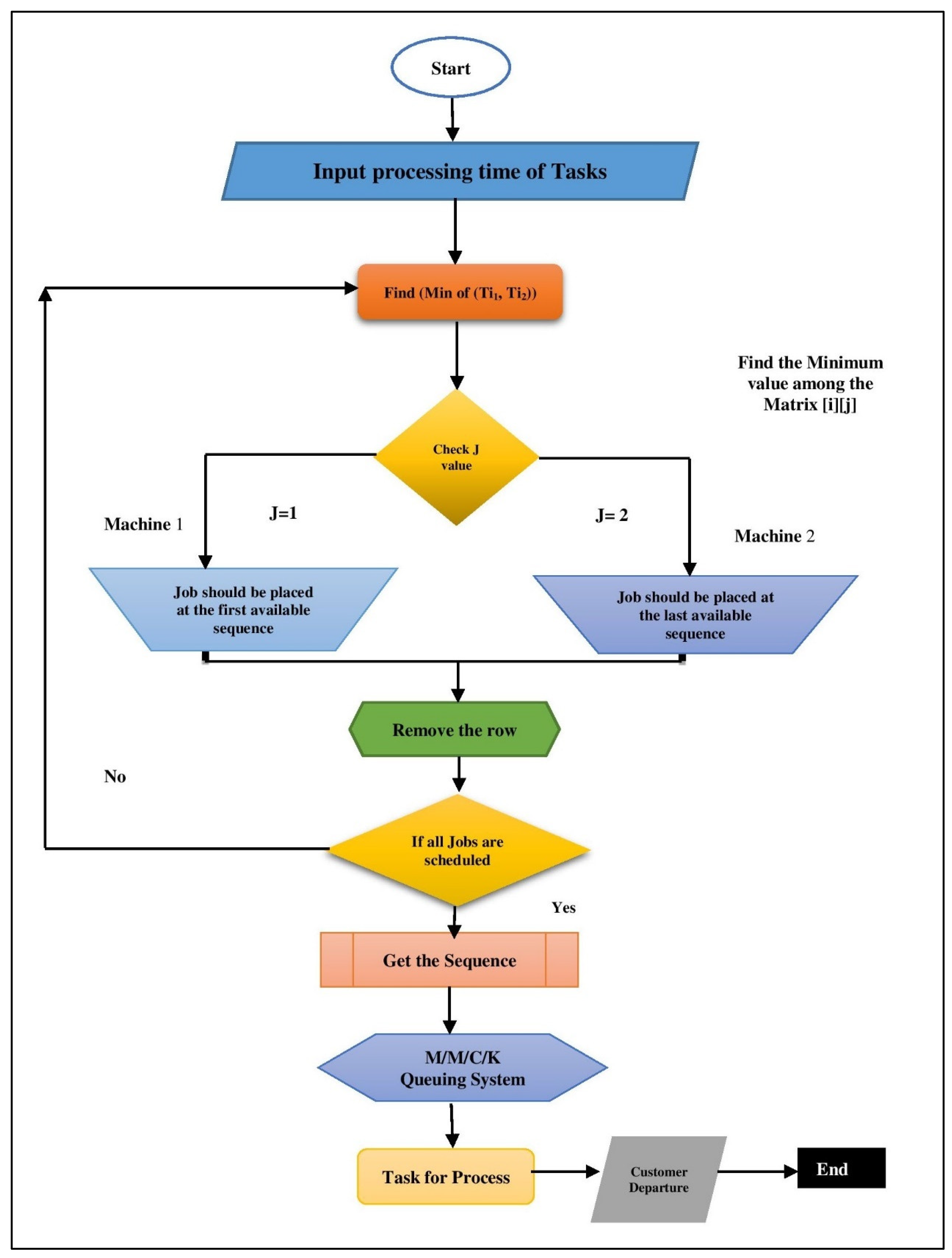
3.3. Johnson Sequencing Algorithm Flowchart
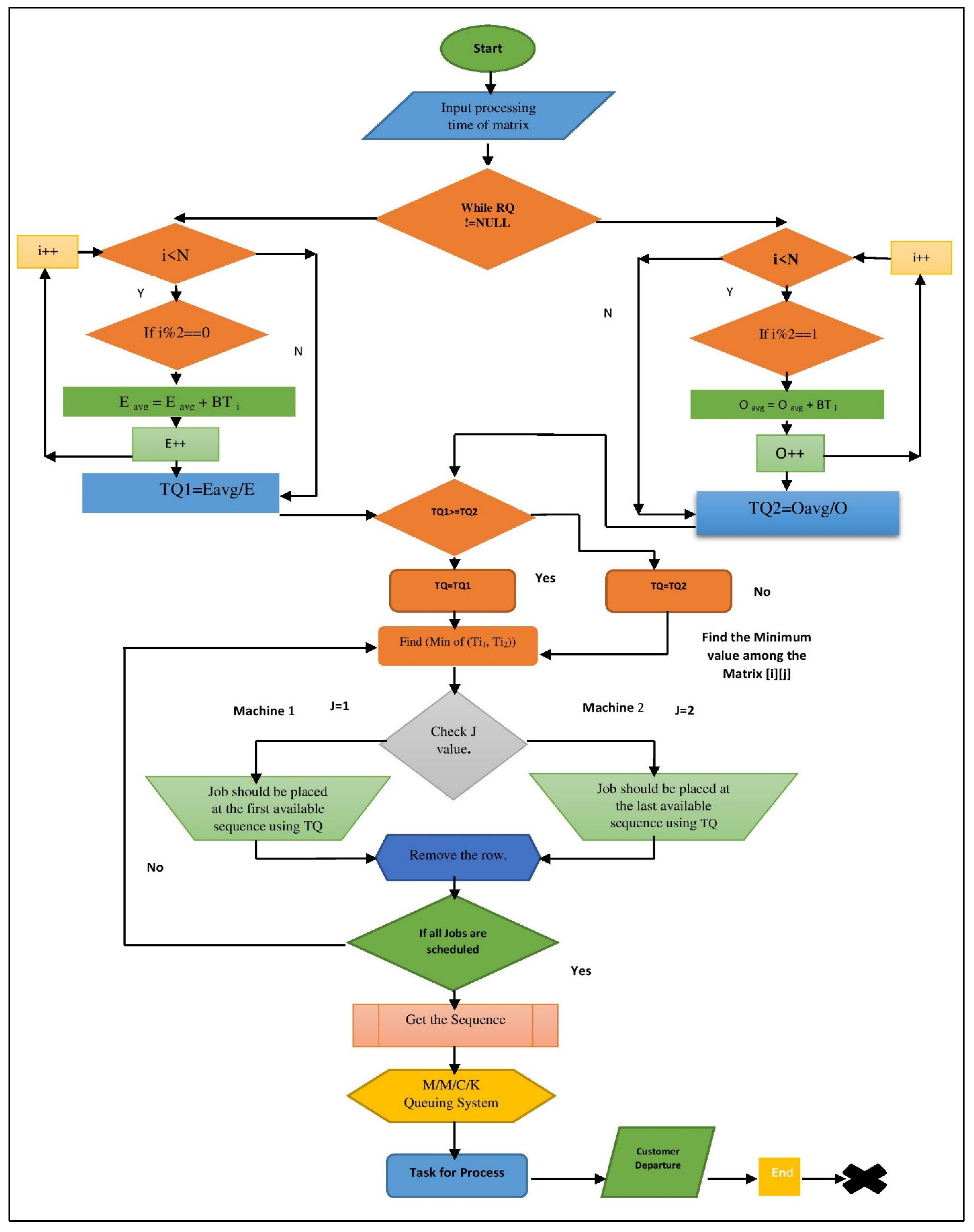
3.4. Dynamic Johnson Sequencing Algorithm Flowchart
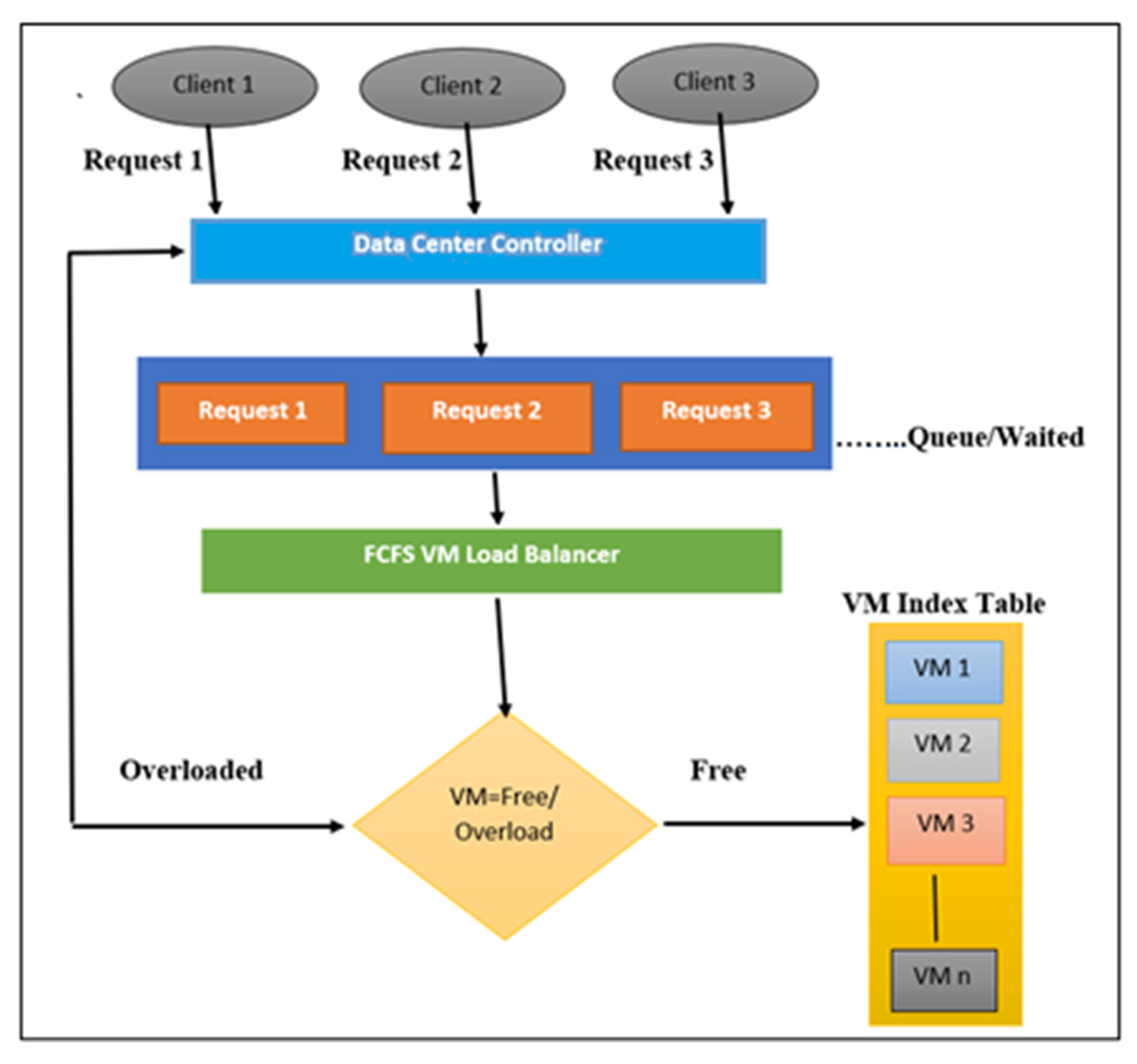
3.5. FCFS Algorithm Flowchart
| Algorithm 1. For Dynamic Johnson Sequencing (DJS) |
| 1 Input ((b11, b21), ((b12, b22),..., ((b1n, b2n)) 2 Output: an optimal schedule σ Step 1 // n= Number of jobs and BT= Jobs Burst Time 3. arr[]=Bt of all tasks waiting in the ready queue 4. repeat for (i=0 to n−1) { Sum1=Sum1+Bti i+=2; }
5. repeat for (j=1 to n− 1) { Sum2=Sum2+Btj; j+=2; }
6. if(Tqe>Tqo) then Tq=Tqe else Tq=Tqo 7. // AssignTq to (1 to n jobs in the queue) for i=0 to n loop ji->Tq 8. J11 ← {Jj∈J: b1j<= b2j}; 9. J22 ← {Jj∈J: b1j> b2j}; Step 2 10. Label this sequence”σ(1)” and place the tasks in J1 in non-decreasing order of the degradation rates b1j; 11. List the occupations in J2 in reverse chronological order of degradation rates b2j; 12. Call this sequence σ(2); Step 3 13. σ ← (σ(1)|σ(2)); 14. Return |
4. Experimental Analysis
4.1. Experimental Analysis of FCFS Using Two Machines
4.2. Experimental Analysis of Johnson Sequencing Using Two Machines

| Tasks | Machine1 | Machine2 | ||
|---|---|---|---|---|
| IN TIME | OUT TIME | IN TIME | OUT TIME | |
| J1 | 0 | 0.08 | 0.08 | 0.19 |
| J2 | 0.08 | 0.21 | 0.21 | 0.35 |
| J5 | 0.21 | 0.34 | 0.35 | 0.71 |
| J3 | 0.34 | 0.54 | 0.71 | 0.87 |
| J4 | 0.54 | 0.82 | 0.87 | 1.01 |
4.3. Experimental Analysis of Max–Min Using Two Machines
| Tasks | Machine1 | Machine2 | ||
|---|---|---|---|---|
| IN TIME | OUT TIME | IN TIME | OUT TIME | |
| J1 | 0 | 0.08 | 0.08 | 0.19 |
| J2 | 0.08 | 0.21 | 0.21 | 0.35 |
| J3 | 0.21 | 0.41 | 0.41 | 0.57 |
| J4 | 0.41 | 0.61 | 0.76 | 0.96 |
| J5 | 0.61 | 0.74 | 1.17 | 1.37 |
| J4 | 0.74 | 0.76 | IDLE | IDLE |
| J5 | 1.01 | 1.17 | IDLE | IDLE |
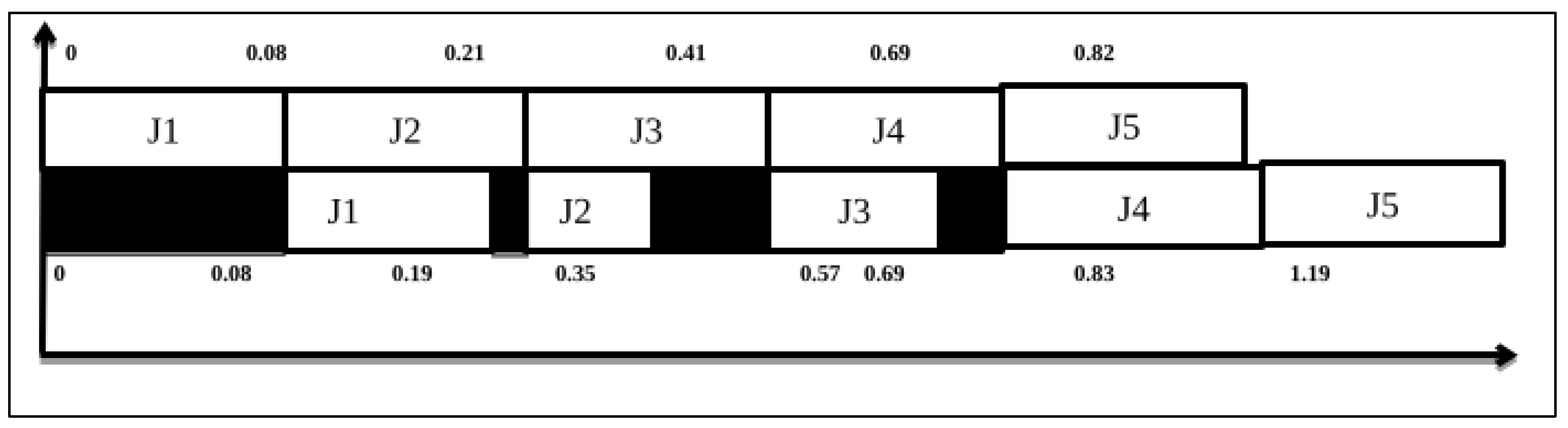
4.4. Experimental Analysis of Dynamic Johnson Sequencing Using Two Machines
| Tasks | Machine1 | Machine2 | ||
|---|---|---|---|---|
| IN TIME | OUT TIME | IN TIME | OUT TIME | |
| J1 | 0 | 0.08 | 0.08 | 0.19 |
| J2 | 0.08 | 0.21 | 0.21 | 0.35 |
| J5 | 0.21 | 0.34 | 0.35 | 0.70 |
| J3 | 0.34 | 0.54 | 0.70 | 0.86 |
| J4 | 0.54 | 0.82 | 0.86 | 1.00 |
| J5 | 0.82 | 0.83 | IDLE | IDLE |
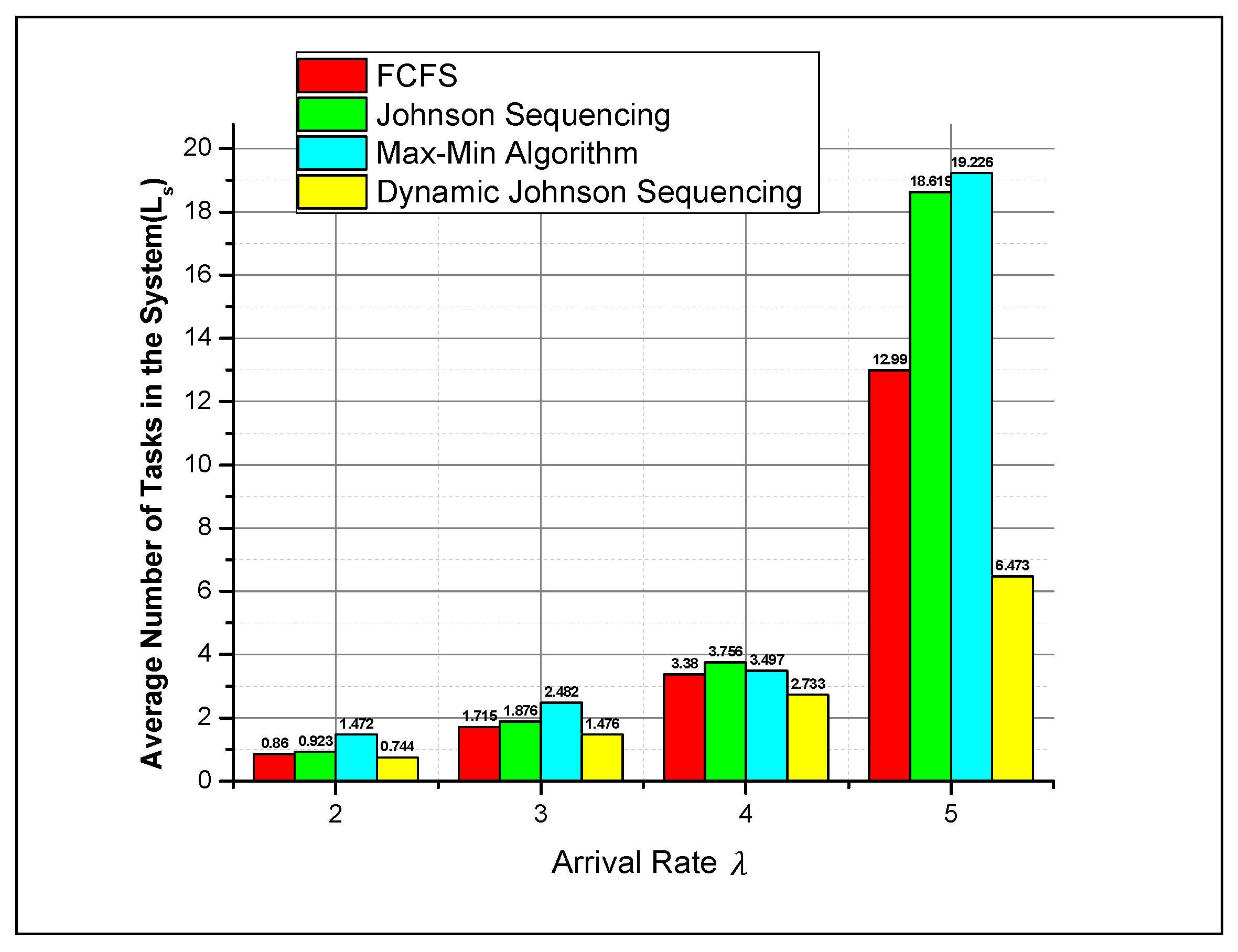
| Lq | Ls | Wq | Ws | |
|---|---|---|---|---|
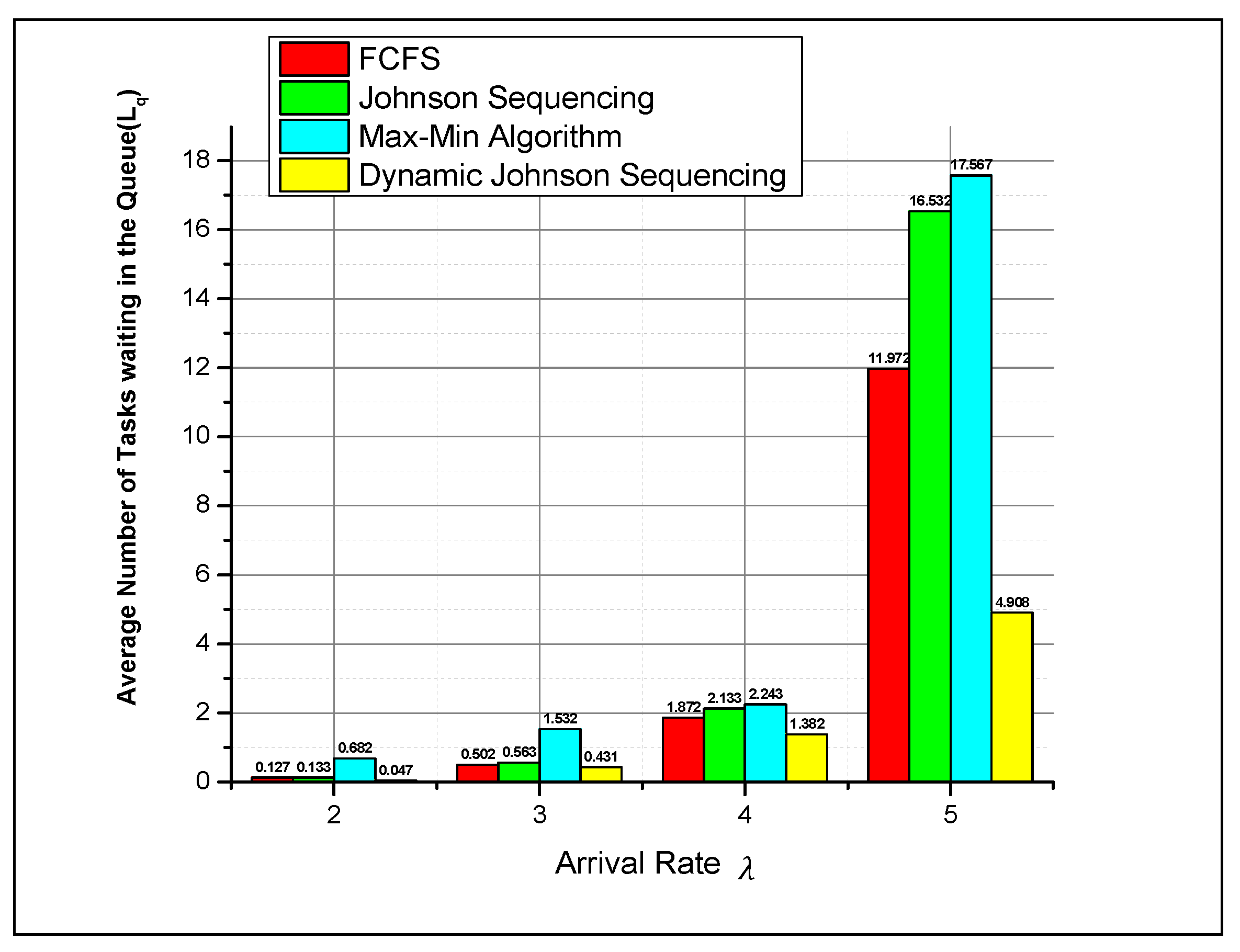
| λ = 2 | 0.127 | 0.860 | 0.058 | 0.428 |
| λ = 3 | 0.502 | 1.715 | 0.164 | 0.534 |
| λ = 4 | 1.872 | 3.380 | 0.447 | 0.817 |
| λ = 5 | 11.972 | 12.990 | 2.198 | 2.568 |
| Lq | Ls | Wq | Ws | |
|---|---|---|---|---|
| λ = 2 | 0.133 | 0.923 | 0.063 | 0.441 |
| λ = 3 | 0.563 | 1.876 | 0.18 | 0.558 |
| λ = 4 | 2.133 | 3.756 | 0.51 | 0.888 |
| λ = 5 | 16.532 | 18.619 | 3.285 | 3.663 |
| Lq | Ls | Wq | Ws | |
|---|---|---|---|---|
| λ = 2 | 0.682 | 1.472 | 0.347 | 0.693 |
| λ = 3 | 1.532 | 2.482 | 0.497 | 0.873 |
| λ = 4 | 2.243 | 3.497 | 0.552 | 0.898 |
| λ = 5 | 17.567 | 19.226 | 4.095 | 40.443 |
| Lq | Ls | Wq | Ws | |
|---|---|---|---|---|
| λ = 2 | 0.047 | 0.744 | 0.025 | 0.377 |
| λ = 3 | 0.431 | 1.476 | 0.141 | 0.448 |
| λ = 4 | 1.382 | 2.733 | 0.337 | 0.695 |
| λ = 5 | 4.908 | 6.473 | 0.950 | 1.386 |
5. Result and Discussion


6. Statistical Analysis Using t-Test


7. Conclusions
- Resource utilization:When compared to FCFS, Johnson sequencing, and max–min Johnson sequencing, DJS task scheduling maximizes the use of cloud resources, such as virtual machines and storage, by allocating tasks to available resources based on their requirements and priorities.
- Performance enhancement: When compared to FCFS, Johnson sequencing, and max–min Johnson sequencing, DJS scheduling algorithms have lower reaction times, higher throughput, and lower latency, which can enhance the overall performance of cloud applications.
- Cost management: Task scheduling techniques that effectively allocate resources and reduce over-provisioning can aid in cost control. For businesses trying to optimize their cloud schedule, this is especially crucial. As a result, DJS scheduling techniques are more cost-effective than FCFS, Johnson sequencing, and max–min Johnson sequencing.
- Load balancing: Task scheduling aids in load balancing by equally spreading loads among resources that are at hand, avoiding resource bottlenecks, and making sure that no resource is overloaded. Therefore, DJS optimizes the load such that jobs coming in are completed within a certain time quantum that is estimated using the even–odd round-robin scheduling approach.
- Fault tolerance: by intelligently moving jobs in the event of resource failures or deterioration, the DJS scheduling approach may improve the fault tolerance and dependability of cloud systems.
- Complexity: Because of the dynamic nature of cloud resources, a wide range of workloads, and various user expectations, scheduling in a cloud environment can be challenging. To manage this complexity, an advanced dynamic Johnson sequencing technique is required.
- Compliance with QoS and SLAs: To ensure that applications satisfy performance guarantees and provide the anticipated quality of service, task scheduling must take into account QoS requirements and servicequality agreements (SLAs). In terms of QoS and SLA compliance, DJS is therefore the best option.
Author Contributions
Funding
Conflicts of Interest
References
- Talukder, M.K.; Buyya, R. Multiobjective differential evolution for scheduling workflow applications on global grids. Concurr. Comput. Pract. Exp. 2009, 21, 1742–1756. [Google Scholar] [CrossRef]
- Banerjee, P.; Tiwari, A.; Kumar, B.; Thakur, K.; Singh, A.; Dehury, M.K. Task Scheduling in cloud using Heuristic Technique. In Proceedings of the 2023 7th International Conference on Trends in Electronics and Informatics (ICOEI), Tirunelveli, India, 11–13 April 2023; IEEE: Piscataway, NJ, USA, 2023; pp. 709–716. [Google Scholar]
- Baranwal, G.; Vidyarthi, D.P. A fair multi-attribute combinatorial double auction model for resource allocation in cloud computing. J. Syst. Softw. 2015, 108, 60–76. [Google Scholar] [CrossRef]
- Karthick, A.V.; Ramaraj, E.; Subramanian, R.G. An Efficient Multi Queue Job Scheduling for Cloud Computing. In Proceedings of the World Congress on Computing and Communication Technologies (WCCCT), Trichirappalli, India, 27 February–1 March 2014; IEEE: Piscataway, NJ, USA, 2014; pp. 164–166. [Google Scholar]
- Alkhashai, H.M.; Omara, F.A. An Enhanced Task Scheduling Algorithm on Cloud Computing Environment. Int. J. Grid Distrib. Comput. 2016, 9, 91–100. [Google Scholar] [CrossRef]
- Banerjee, P.; Roy, S. An Investigation of Various Task Allocating Mechanism in Cloud. In Proceedings of the 2021 5th International Conference on Information Systems and Computer Networks (ISCON), Mathura, India, 22–23 October 2021; IEEE: Piscataway, NJ, USA, 2021; pp. 1–6. [Google Scholar]
- Barrett, E.; Howley, E.; Duggan, J. A learning architecture for scheduling workflow applications in the cloud. In Proceedings of the Ninth IEEE European Conference on Web Services (ECOWS), Lugano, Switzerland, 14–16 September 2011; pp. 83–90. [Google Scholar]
- Cheng, C.; Li, J.; Wang, Y. An energy-saving task scheduling strategy based on vacation queuing theory in cloud computing. Tsinghua Sci. Technol. 2015, 20, 28–39. [Google Scholar] [CrossRef]
- Lin, C.-C.; Liu, P.; Wu, J.-J. Energy-efficient Virtual Machine Provision Algorithms for Cloud Systems. In Proceedings of the 2011 Fourth IEEE International Conference on Utility and Cloud Computing, Melbourne, Australia, 5–8 December 2011; pp. 81–88. [Google Scholar]
- Delavar, A.G.; Javanmard, M.; Shabestari, M.B.; Talebi, M.K. RSDC (Reliable scheduling distributed in cloud computing). Int. J. Comput. Sci. Eng. Appl. 2012, 2, 1–16. [Google Scholar] [CrossRef]
- Ding, J.; Zhang, Z.; Ma, R.T.; Yang, Y. Auction-based cloud service differentiation with service level objectives. Comput. Netw. 2016, 94, 231–249. [Google Scholar] [CrossRef]
- El-Sayed, T.E.; El-Desoky, A.I.; Al-Rahamawy, M.F. Extended maxmin scheduling using Petri net and load balancing. Int. J. Soft Comput. Eng. 2012, 2, 198–203. [Google Scholar]
- Shaikh, F.B.; Haider, S. Security threats in cloud computing. In Proceedings of the 6th International IEEE Conference on Internet Technology and Secured Transaction, Abu Dhabi, United Arab Emirates, 11–14 December 2012; pp. 214–219. [Google Scholar]
- Gan, G.; Huang, T.; Gao, S. Genetic simulated annealing algorithm for task scheduling based on cloud computing environment. In Proceedings of the IEEE International Conference on Intelligent Computing and Integrated Systems (ICISS), Guilin, China, 22–24 October 2010; pp. 60–63. [Google Scholar]
- Ge, J.W.; Yuan, Y.S. Research of cloud computing task scheduling algorithm based on improved genetic algorithm. Appl. Mech. Mater. 2013, 347, 2426–2429. [Google Scholar] [CrossRef]
- Khazaei, H.; Misic, J.; Misic, V.B. Performance Analysis of Cloud Computing Centers Using M/G/m/m+rQueuing Systems. IEEE Trans. Parallel Distrib. Syst. 2012, 23, 936–943. [Google Scholar] [CrossRef]
- Khazaei, H.; Misic, J.; Misic, V.B. Modelling of Cloud Computing Centers Using M/G/m Queues. In Proceedings of the 31st IEEE International Conference on Distributed Computing Systems Workshops (ICDCSW), Minneapolis, MN, USA, 20–24 June 2011; pp. 87–92. [Google Scholar]
- Liu, H.; Jin, H.; Liao, X.; Hu, L.; Yu, C. Live migration of virtual machine based on full system trace and replay. In Proceedings of the 18th ACM International Symposium on High Performance Distributed Computing, Garching, Germany, 11–13 June 2009; pp. 101–110. [Google Scholar]
- Himthani, P.; Saxena, A.; Manoria, M. Comparative Analysis of VM Scheduling Algorithms in Cloud Environment. Int. J. Comput. Appl. 2015, 120, 1–6. [Google Scholar] [CrossRef]
- Gu, J.; Hu, J.; Zhao, T.; Sun, G. A New Resource Scheduling Strategy Based on Genetic Algorithm in Cloud Computing Environment. J. Comput. 2012, 7, 42–52. [Google Scholar] [CrossRef]
- Ye, K.; Jiang, X.; Ye, D.; Huang, D. Two Optimization Mechanisms to Improve the Isolation Property of Server Consolidation in Virtualized Multi-core Server. In Proceedings of the 12th IEEE International Conference on Performance Computing and Communications, Melbourne, Australia, 1–3 September 2010; pp. 281–288. [Google Scholar]
- Bebortta, S.; Tripathy, S.S.; Modibbo, U.M.; Ali, I. An optimal fog-cloud offloading framework for big data optimization in heterogeneous IoT networks. Decis. Anal. J. 2023, 8, 100295. [Google Scholar] [CrossRef]
- Kalra, M.; Singh, S. A review of metaheuristic scheduling techniques in cloud computing. Egypt. Inform. J. 2015, 16, 275–295. [Google Scholar] [CrossRef]
- Kumar, K.; Hans, A.; Sharma, A.; Singh, N. A Review on Scheduling Issues in Cloud Computing. In Proceedings of the International Conference on Advancements in Engineering and Technology (ICAET 2015), Incheon, Republic of Korea, 11–13 December 2015; pp. 4–7. [Google Scholar]
- Kumar, N.; Sankar, S.G.; Kumar, M.N.; Manikanta, P.; Aravind, V.S. Enhanced Real-Time Group Auction System for Efficient Allocation of Cloud Internet Applications. IJITR 2016, 4, 2836–2840. [Google Scholar]
- Kuo, R.J.; Cheng, C. Hybrid meta-heuristic algorithm for job shop scheduling with due date time window and release time. Int. J. Adv. Manuf. Technol. 2013, 67, 59–71. [Google Scholar] [CrossRef]
- Lee, C.; Wang, P.; Niyato, D. A real-time group auction system for efficient allocation of cloud internet applications. IEEE Trans. Serv. Comput. 2015, 8, 251–268. [Google Scholar] [CrossRef]
- Hines, M.; Gopalan, K. Post-copy based live virtual machine migration using adaptive pre-paging and dynamic selfballooning. In Proceedings of the 2009 ACM SIGPLAN/SIGOPS International Conference on Virtual Execution Environments, Washington, DC, USA, 11–13 March 2009; pp. 51–60. [Google Scholar]
- Mangla, N.; Singh, M.; Rana, S.K. Resource Scheduling In Cloud Environment: A Survey. Advances in Science and Technology. Res. J. 2016, 10, 38–50. [Google Scholar]
- Schmidt, M.; Fallenbeck, N.; Smith, M.; Freisleben, B. Efficient Distribution of Virtual Machines for Cloud Computing. In Proceedings of the Parallel, Distributed and Network-Based Processing (PDP), 2010 18th Euromicro International Conference, Pisa, Italy, 17–19 February 2010; pp. 567–574. [Google Scholar]
- Mishra, R.K.; Kumar, S.; Naik, S.B. Priority based round-Robin service broker algorithm for cloud-analyst. In Proceedings of the International Advance Computing Conference (IACC), Gurgaon, India, 21–22 February 2014; IEEE: Piscataway, NJ, USA, 2014; pp. 878–881. [Google Scholar]
- Nejad, M.M.; Mashayekhy, L.; Grosu, D. Truthful greedy mechanisms for dynamic virtual machine provisioning and allocation in clouds. IEEE Trans. Parallel Distrib. Syst. 2015, 26, 594–603. [Google Scholar] [CrossRef]
- Poola, D.; Ramamohanarao, K.; Buyya, R. Fault-tolerant workflow scheduling using spot instances on clouds. Proc. Comput. Sci. 2014, 29, 523–533. [Google Scholar] [CrossRef]
- Jansen, R.; Brenner, P.R. Energy Efficient Virtual Machine Allocation in the Cloud. In Proceedings of the 2011 International Green Computing Conference and Workshops (IGCC), Orlando, FL, USA, 25–28 July 2011; pp. 1–8. [Google Scholar]
- Pal, S.; Pattnaik, P.K. Efficient architectural Framework of Cloud Computing. Int. J. Cloud Comput. Serv. Sci. 2012, 1, 66–73. [Google Scholar] [CrossRef]
- Sundareswaran, S.; Squicciarini, A.; Lin, D. A Brokerage-Based Approach for Cloud Service Selection. In Proceedings of the 2012 IEEE Fifth International Conference on Cloud Computing, Honolulu, HI, USA, 24–29 June 2012; IEEE Computer Society: Washington, DC, USA, 2012; pp. 558–565. [Google Scholar]
- Yang, S.; Kwon, D.; Yi, H.; Cho, Y.; Kwon, Y.; Paek, Y. Techniques to Minimize State Transfer Costs for Dynamic Execution Offloading in Mobile Cloud Computing. IEEE Trans. Mob. Comput. 2014, 13, 2648–2659. [Google Scholar] [CrossRef]
- Salot, P. A survey of various scheduling algorithm in cloud computing environment. Int. J. Res. Eng. Technol. 2013, 2, 131–135, ISSN 2319-1163. [Google Scholar]
- Singh, S.; Chana, I. A survey on resource scheduling in cloud computing: Issues and challenges. J. Grid Comput. 2016, 14, 217–264. [Google Scholar] [CrossRef]
- Pal, S.; Mohanty, S.; Pattnaik, P.K.; Mund, G.B. A Virtualization Model for Cloud Computing. In Proceedings of the International Conference on Advances in Computer Science, Delhi, India, 28–29 December 2012; pp. 10–16. [Google Scholar]
- Sowjanya, T.S.; Praveen, D.; Satish, K.; Rahiman, A. The queuing theory in cloud computing to reduce the waiting time. Int. J. Comput. Sci. Eng. Technol. 2011, 1, 110–112. [Google Scholar]
- Szabo, C.; Kroeger, T. Evolving multi-objective strategies for task allocation of scientific workflows on public clouds. In Proceedings of the 2012 IEEE Congress on Evolutionary Computation, Brisbane, Australia, 10–15 June 2012; IEEE: Piscataway, NJ, USA, 2012; pp. 1–8. [Google Scholar]
- Topcuoglu, H.; Hariri, S.; Wu, M.Y. Performance-effective and lowcomplexity task scheduling for heterogeneous computing. IEEE Trans. Parallel Distrib. Syst. 2002, 13, 260–274. [Google Scholar] [CrossRef]
- Sarathy, V.; Narayan, P.; Mikkilineni, R. Next generation cloud computing architecture-enabling real-time dynamism for shared distributed physical infrastructure. In Proceedings of the 19th IEEE International Workshops on Enabling Technologies: Infrastructures for Collaborative Enterprises (WETICE’10), Larissa, Greece, 28–30 June 2010; pp. 48–53. [Google Scholar]
- Yassein, M.O.B.; Khamayseh, Y.M.; Hatamleh, A.M. Intelligent randomize round Robin for cloud computing. Int. J. Cloud Appl. Comput. 2013, 3, 27–33. [Google Scholar] [CrossRef]
- Yu, J.; Kirley, M.; Buyya, R. Multi-objective planning for workflow execution on grids. In Proceedings of the 8th IEEE/ACM International Conference on Grid Computing (GRID ’07), Austin, TX, USA, 19–21 September 2007; pp. 10–17. [Google Scholar]
- Xiao, Z.; Song, W.; Chen, Q. Dynamic Resource Allocation Using Virtual Machines for Cloud Computing Environment. IEEE Trans. Parallel Distrib. Syst. 2013, 24, 1107–1117. [Google Scholar] [CrossRef]
- Zhang, Y.; Li, B.; Huang, Z.; Wang, J.; Zhu, J. SGAM: Strategy-proof group buying-based auction mechanism for virtual machine allocation in clouds. Concurr. Comput. Pract. Exp. 2015, 27, 5577–5589. [Google Scholar] [CrossRef]
- Zhao, W.; Stankovic, J.A. Performance analysis of FCFS and improved FCFS scheduling algorithms for dynamic real-time computer systems. In Proceedings of the Real Time Systems Symposium, Santa Monica, CA, USA, 5–7 December 1989; IEEE: Piscataway, NJ, USA, 1989; pp. 156–165. [Google Scholar]
- Zhu, Z.; Zhang, G.; Li, M.; Liu, X. Evolutionary Multi-Objective Workflow Scheduling in Cloud. IEEE Trans. Parallel Distrib. Syst. 2015, 27, 1344–1357. [Google Scholar] [CrossRef]


| REF. NO | Scheduling Method | Maxspan | Total Processing Time | Completion Time | Turnaround Time |
|---|---|---|---|---|---|
| 1 | Genetic algorithm | Yes | No | Yes | No |
| 2 | Simulated annealing | no | Yes | Yes | yes |
| 3 | Round-robin | Yes | No | Yes | No |
| 4 | Round-robin | No | Yes | No | Yes |
| 5 | Min–min, MaxMin | Yes | No | No | Yes |
| 6 | Meta-heuristic | No | Yes | Yes | No |
| 7 | Reinforcement learning | Yes | No | Yes | No |
| 15 | Ant colony method | No | Yes | No | No |
| 18 | Priority-based job-scheduling algorithm | Yes | Yes | Yes | No |
| 19 | Dens | Yes | No | Yes | No |
| 20 | Multi-homing | Yes | Yes | Yes | No |
| Task | S1 Processing Time | S2 Processing Time | Total Burst Time |
|---|---|---|---|
| Task1 | J1.1 | J1.2 | Bt1 |
| Jask2 | J2.1 | J2.2 | Bt2 |
| Jask3 | J3.1 | J3.2 | Bt3 |
| Jask4 | J4.1 | J4.2 | Bt4 |
| Jask5 | J5.1 | J5.2 | Bt5 |
| Tasks | Processing Time of Server Machine 1 (in Milliseconds) | Processing Time of Server Machine 2 (in Milliseconds) | Total Burst Time of Tasks (in Milliseconds) |
|---|---|---|---|
| J1 | 0.08 | 0.11 | 0.19 |
| J2 | 0.13 | 0.14 | 0.27 |
| J3 | 0.20 | 0.16 | 0.36 |
| J4 | 0.28 | 0.14 | 0.42 |
| J5 | 0.13 | 0.36 | 0.49 |
| Tasks | Machine1 | Machine2 | ||
|---|---|---|---|---|
| IN TIME | OUT TIME | IN TIME | OUT TIME | |
| J1 | 0 | 0.08 | 0.08 | 0.19 |
| J2 | 0.08 | 0.21 | 0.21 | 0.35 |
| J3 | 0.21 | 0.41 | 0.41 | 0.57 |
| J4 | 0.41 | 0.69 | 0.69 | 0.83 |
| J5 | 0.69 | 0.82 | 0.83 | 1.19 |
| Lq (Average Number of Jobs in the Queue) | Mean | Std. Deviation | Std. Error Mean | |
|---|---|---|---|---|
| Pair 1 | FCFS(2 Server) | 3.618250 | 5.6194415 | 2.8097208 |
| DJS(2 Server) | 1.692000 | 2.2162207 | 1.1081103 | |
| Pair 1 | JS(2 Server) | 4.840250 | 7.8417534 | 3.9208767 |
| DJS(2 Server) | 1.692000 | 2.2162207 | 1.1081103 | |
| Pair 1 | Max–Min(2 Server) | 5.506000 | 8.0659478 | 4.0329739 |
| DJS(2 Server) | 1.692000 | 2.2162207 | 1.1081103 | |
| Lq (Average Number of Jobs in the Queue) | Correlation | Sig. | |
|---|---|---|---|
| Pair 1 | FCFS(2 Server) and DJS(2 Server) | 0.992 | 0.008 |
| Pair 1 | JS(2 Server) and DJS(2 Server) | 0.989 | 0.011 |
| Pair 1 | Max–Min(2 Server) and DJS(2 Server) | 0.984 | 0.016 |
| Lq (Average Number of Jobs in the Queue) | Paired Differences | t-Test Value | |||||
|---|---|---|---|---|---|---|---|
| Mean | Std. Deviation | Std. Error Mean | 50% Confidence Interval of the Difference | ||||
| Lower | Upper | ||||||
| Pair 1 | FCFS(2 Server)–DJS(2 Server) | 1.9262500 | 3.4307376 | 1.7153688 | 0.6141776 | 3.2383224 | 1.123 |
| Pair 1 | JS(2 Server)–DJS(2 Server) | 3.1482500 | 5.6586301 | 2.8293151 | 0.9841286 | 5.3123714 | 1.113 |
| Pair 1 | Max–Min(2 Server)–DJS(2 Server) | 3.8140000 | 5.8997357 | 2.9498679 | 1.5576687 | 6.0703313 | 1.293 |
| Mean | Std. Deviation | Std. Error Mean | ||
|---|---|---|---|---|
| Pair 1 | FCFS(2 Server) | 4.736250 | 5.6011031 | 2.8005516 |
| DJS(2 Server) | 2.856500 | 2.5470742 | 1.2735371 | |
| Pair 1 | JS(2 Server) | 6.293500 | 8.3008721 | 4.1504361 |
| DJS(2 Server) | 2.856500 | 2.5470742 | 1.2735371 | |
| Pair 1 | Max–Min(2 Server) | 6.669250 | 8.4118886 | 4.2059443 |
| DJS(2 Server) | 2.856500 | 2.5470742 | 1.2735371 | |
| Lq (Average Number of Jobs in the Queue) | Correlation | Sig. | |
|---|---|---|---|
| Pair 1 | FCFS(2 Server) and DJS(2 Server) | 0.990 | 0.010 |
| Pair 1 | JS(2 Server) and DJS(2 Server) | 0.983 | 0.017 |
| Pair 1 | Max–Min(2 Server) and DJS(2 Server) | 0.973 | 0.027 |
| Paired Differences | t-Test Value | ||||||
|---|---|---|---|---|---|---|---|
| Mean | Std. Deviation | Std. Error Mean | 50% Confidence Interval of the Difference | ||||
| Lower | Upper | ||||||
| Pair 1 | FCFS(2 Server)–DJS(2 Server) | 1.8797500 | 3.0998191 | 1.5499095 | 0.6942361 | 3.0652639 | 1.213 |
| Pair 1 | JS(2 Server)–DJS(2 Server) | 3.4370000 | 5.8169869 | 2.9084935 | 1.2123157 | 5.6616843 | 1.182 |
| Pair 1 | Max–Min(2 Server)–DJS(2 Server) | 3.8127500 | 5.9614449 | 2.9807224 | 1.5328183 | 6.0926817 | 1.279 |
| Mean | Std. Deviation | Std. Error Mean | ||
| Pair 1 | FCFS(2 Server) | 0.716750 | 1.0010579 | 0.5005289 |
| DJS(2 Server) | 0.363250 | 0.4118142 | 0.2059071 | |
| Pair 1 | JS(2 Server) | 1.009500 | 1.5287613 | 0.7643806 |
| DJS(2 Server) | 0.363250 | 0.4118142 | 0.2059071 | |
| Pair 1 | Max–Min(2 Server) | 1.372750 | 1.8169000 | 0.9084500 |
| DJS(2 Server) | 0.363250 | 0.4118142 | 0.2059071 | |
| Ls (Average Number of Jobs in the Queue) | Correlation | Sig. | |
|---|---|---|---|
| Pair 1 | FCFS(2 Server) and DJS(2 Server) | 0.988 | 0.012 |
| Pair 1 | JS(2 Server) and DJS(2 Server) | 0.981 | 0.019 |
| Pair 1 | Max–Min(2 Server) and DJS(2 Server) | 0.962 | 0.038 |
| Paired Differences | t-Test Value | ||||||
|---|---|---|---|---|---|---|---|
| Mean | Std. Deviation | Std. Error Mean | 50% Confidence Interval of the Difference | ||||
| Lower | Upper | ||||||
| Pair 1 | FCFS(2 Server)–DJS(2 Server) | 0.3535000 | 0.5975988 | 0.2987994 | 0.1249506 | 0.5820494 | 1.183 |
| Pair 1 | JS(2 Server)–DJS(2 Server) | 0.6462500 | 1.1276174 | 0.5638087 | 0.2149971 | 1.0775029 | 1.146 |
| Pair 1 | Max–Min(2 Server)–DJS(2 Server) | 1.0095000 | 1.4249338 | 0.7124669 | 0.4645395 | 1.5544605 | 1.417 |
| Mean | Std. Deviation | Std. Error Mean | ||
|---|---|---|---|---|
| Pair 1 | FCFS(2 Server) | 1.086750 | 1.0010579 | 0.5005289 |
| DJS(2 Server) | 0.726500 | 0.4603061 | 0.2301530 | |
| Pair 1 | JS(2 Server) | 1.387500 | 1.5287613 | 0.7643806 |
| DJS(2 Server) | 0.726500 | 0.4603061 | 0.2301530 | |
| Pair 1 | Max–Min(2 Server) | 1.726750 | 1.8131344 | 0.9065672 |
| DJS(2 Server) | 0.726500 | 0.4603061 | 0.2301530 | |
| Lq (Average Number of Jobs in the Queue) | Correlation | Sig. | |
|---|---|---|---|
| Pair 1 | FCFS(2 Server) and DJS(2 Server) | 0.991 | 0.009 |
| Pair 1 | JS(2 Server) and DJS(2 Server) | 0.984 | 0.016 |
| Pair 1 | Max–Min(2 Server) and DJS(2 Server) | 0.965 | 0.035 |
| Paired Differences | t-Test Value | ||||||
|---|---|---|---|---|---|---|---|
| Mean | Std. Deviation | Std. Error Mean | 50% Confidence Interval of the Difference | ||||
| Lower | Upper | ||||||
| Pair 1 | FCFS(2 Server)–DJS(2 Server) | 0.3602500 | 0.5485997 | 0.2742998 | 0.1504402 | 0.5700598 | 1.313 |
| Pair 1 | JS(2 Server)–DJS(2 Server) | 0.6610000 | 1.0786550 | 0.5393275 | 0.2484725 | 1.0735275 | 1.226 |
| Pair 1 | Max–Min(2 Server)–DJS(2 Server) | 1.0002500 | 1.3741590 | 0.6870795 | 0.4747082 | 1.5257918 | 1.456 |
Disclaimer/Publisher’s Note: The statements, opinions and data contained in all publications are solely those of the individual author(s) and contributor(s) and not of MDPI and/or the editor(s). MDPI and/or the editor(s) disclaim responsibility for any injury to people or property resulting from any ideas, methods, instructions or products referred to in the content. |
© 2023 by the authors. Licensee MDPI, Basel, Switzerland. This article is an open access article distributed under the terms and conditions of the Creative Commons Attribution (CC BY) license (https://creativecommons.org/licenses/by/4.0/).
Share and Cite
Banerjee, P.; Roy, S.; Modibbo, U.M.; Pandey, S.K.; Chaudhary, P.; Sinha, A.; Singh, N.K. OptiDJS+: A Next-Generation Enhanced Dynamic Johnson Sequencing Algorithm for Efficient Resource Scheduling in Distributed Overloading within Cloud Computing Environment. Electronics 2023, 12, 4123. https://doi.org/10.3390/electronics12194123
Banerjee P, Roy S, Modibbo UM, Pandey SK, Chaudhary P, Sinha A, Singh NK. OptiDJS+: A Next-Generation Enhanced Dynamic Johnson Sequencing Algorithm for Efficient Resource Scheduling in Distributed Overloading within Cloud Computing Environment. Electronics. 2023; 12(19):4123. https://doi.org/10.3390/electronics12194123
Chicago/Turabian StyleBanerjee, Pallab, Sharmistha Roy, Umar Muhammad Modibbo, Saroj Kumar Pandey, Parul Chaudhary, Anurag Sinha, and Narendra Kumar Singh. 2023. "OptiDJS+: A Next-Generation Enhanced Dynamic Johnson Sequencing Algorithm for Efficient Resource Scheduling in Distributed Overloading within Cloud Computing Environment" Electronics 12, no. 19: 4123. https://doi.org/10.3390/electronics12194123
APA StyleBanerjee, P., Roy, S., Modibbo, U. M., Pandey, S. K., Chaudhary, P., Sinha, A., & Singh, N. K. (2023). OptiDJS+: A Next-Generation Enhanced Dynamic Johnson Sequencing Algorithm for Efficient Resource Scheduling in Distributed Overloading within Cloud Computing Environment. Electronics, 12(19), 4123. https://doi.org/10.3390/electronics12194123