
Research on the Three-Dimensional Electromagnetic Positioning Method Based on Spectrum Line Interpolation


Abstract
:1. Introduction
2. Theoretical Analysis
2.1. Theoretical Foundation
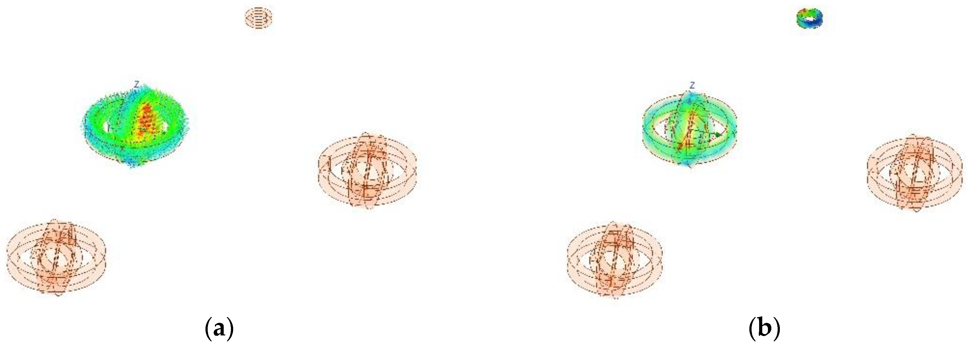
2.1.1. Magnetic Dipole Model
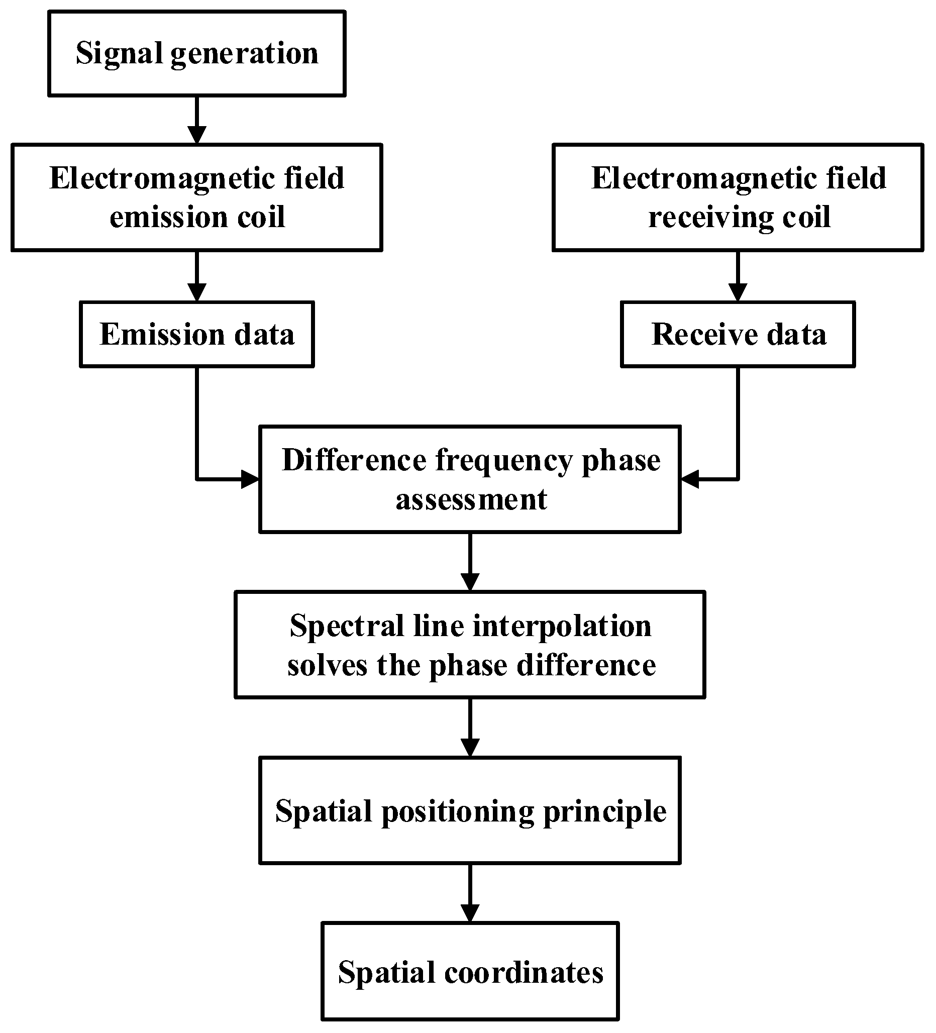
2.1.2. Phase-Based Three-Dimensional Electromagnetic Positioning Principle
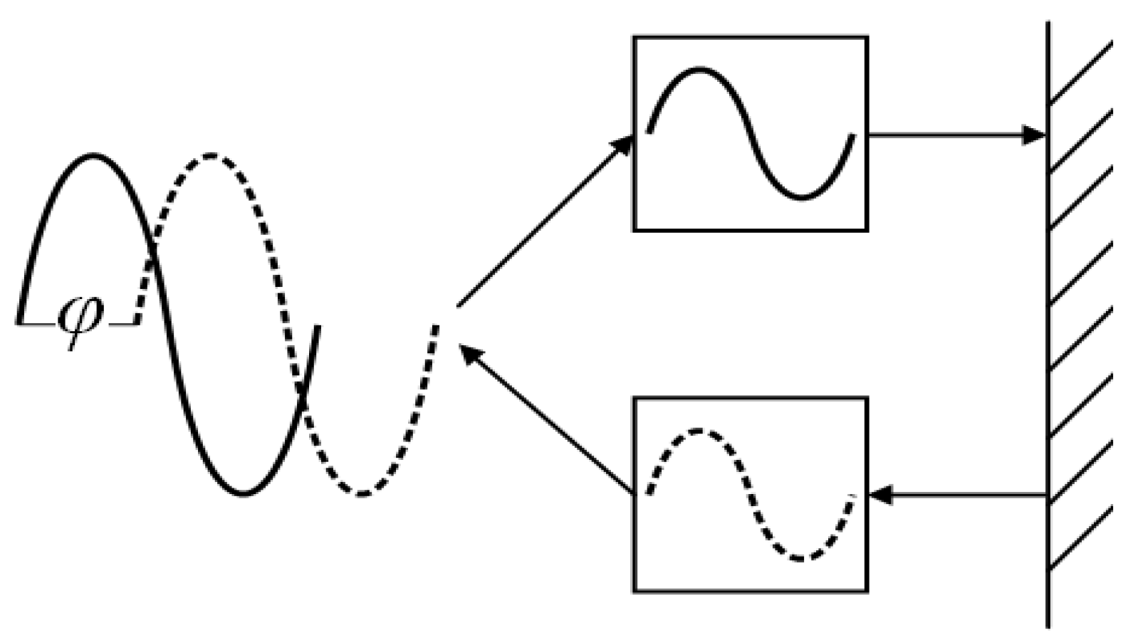
Phase Ranging Principle
The Determination of the Measurement Frequency for the Ruler
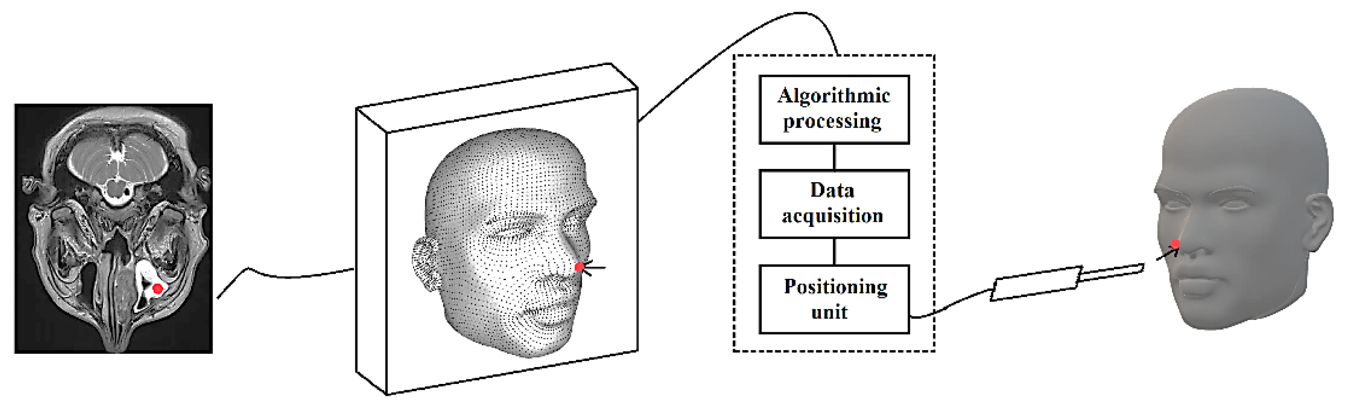
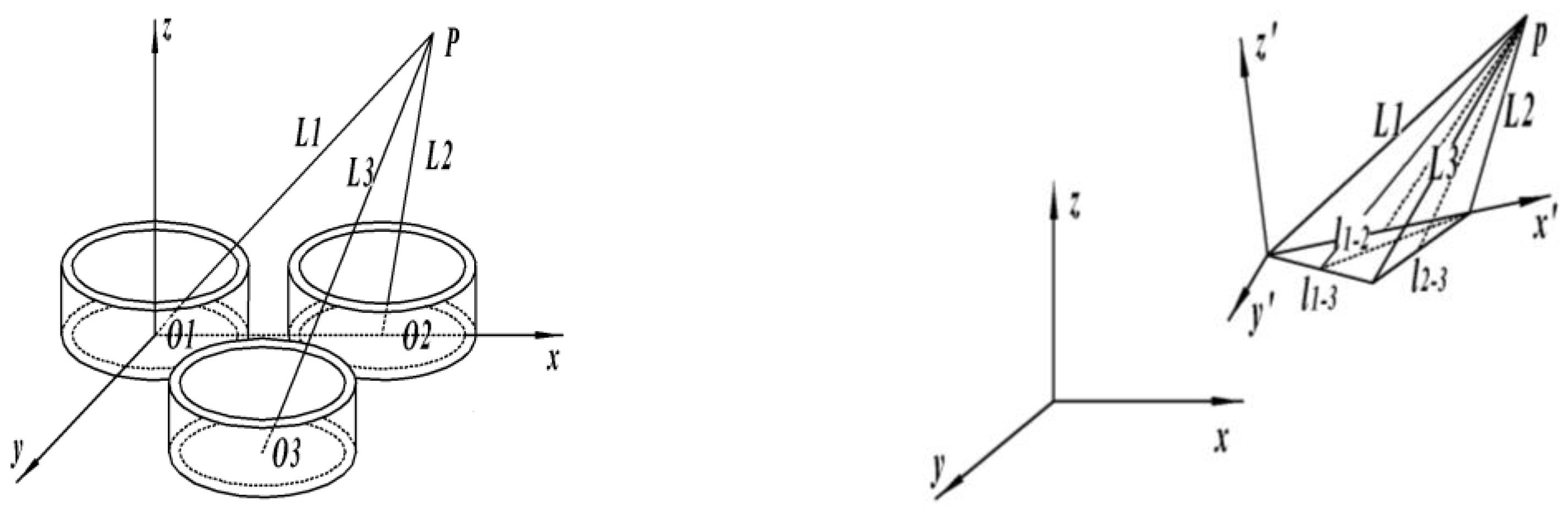
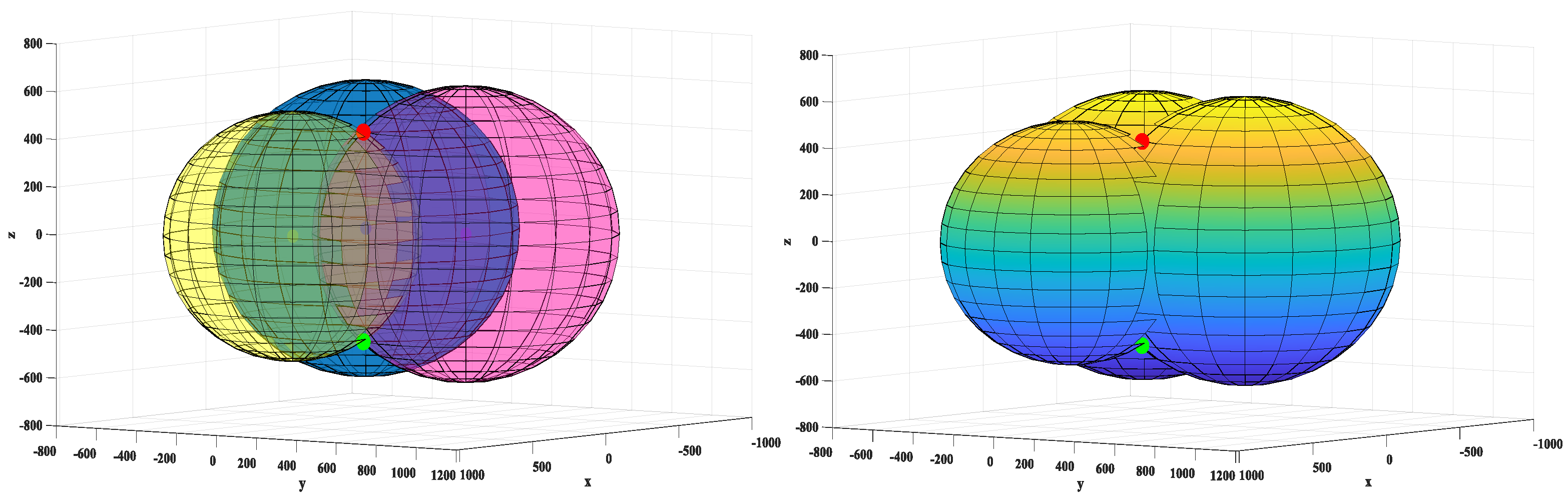
Positioning Principle
2.2. Key Technology Research
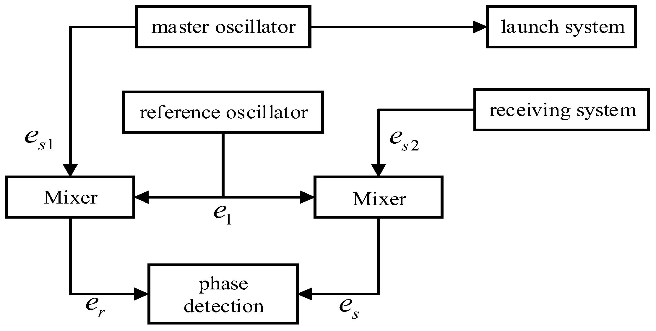
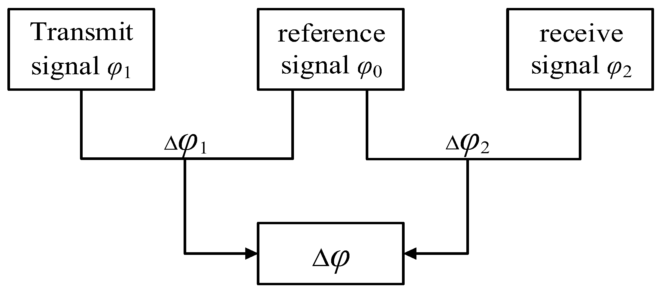
2.2.1. Differential Frequency Phase Detection Technique
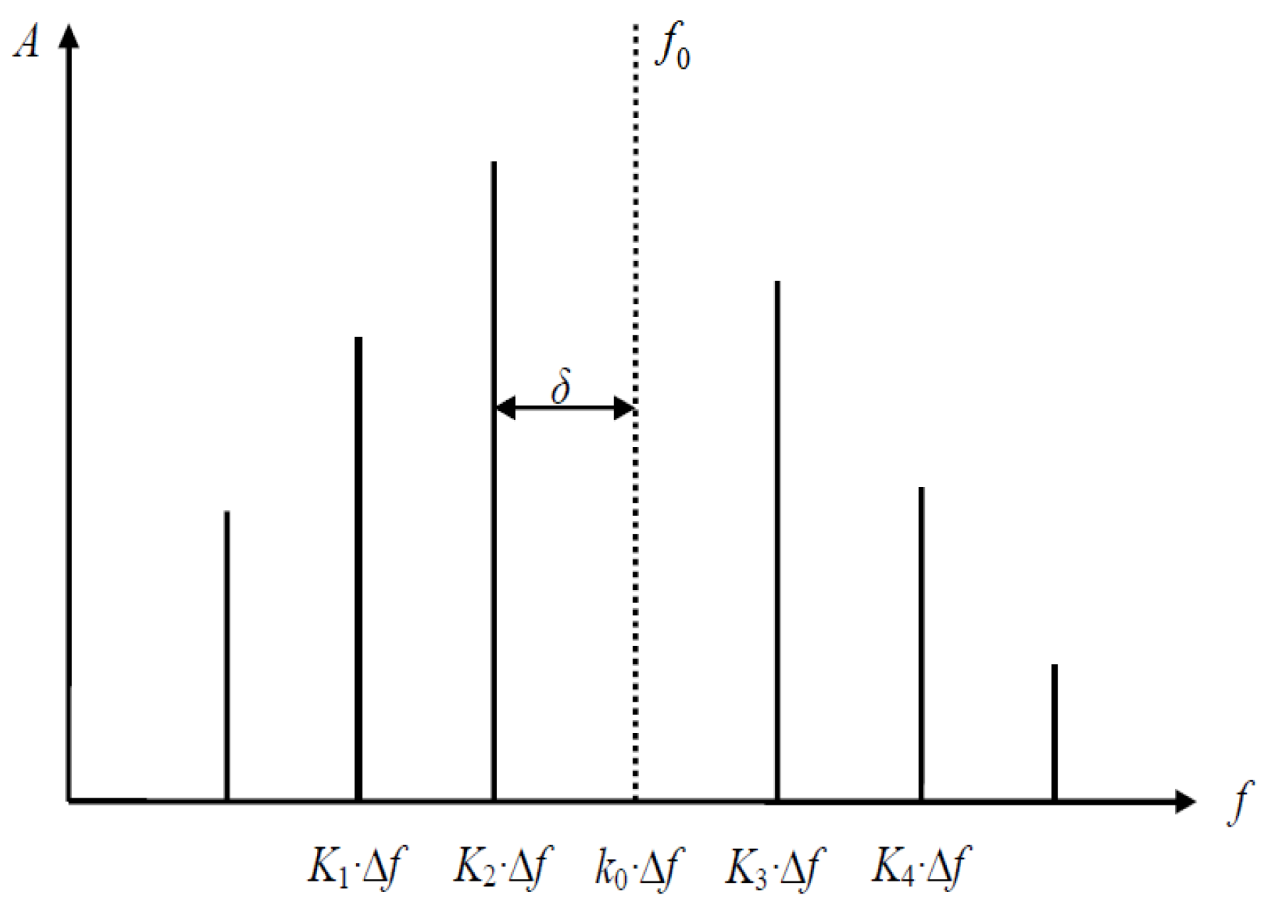
2.2.2. Phase Difference Calculation Algorithm
3. Experiment and Experimental Result Analysis
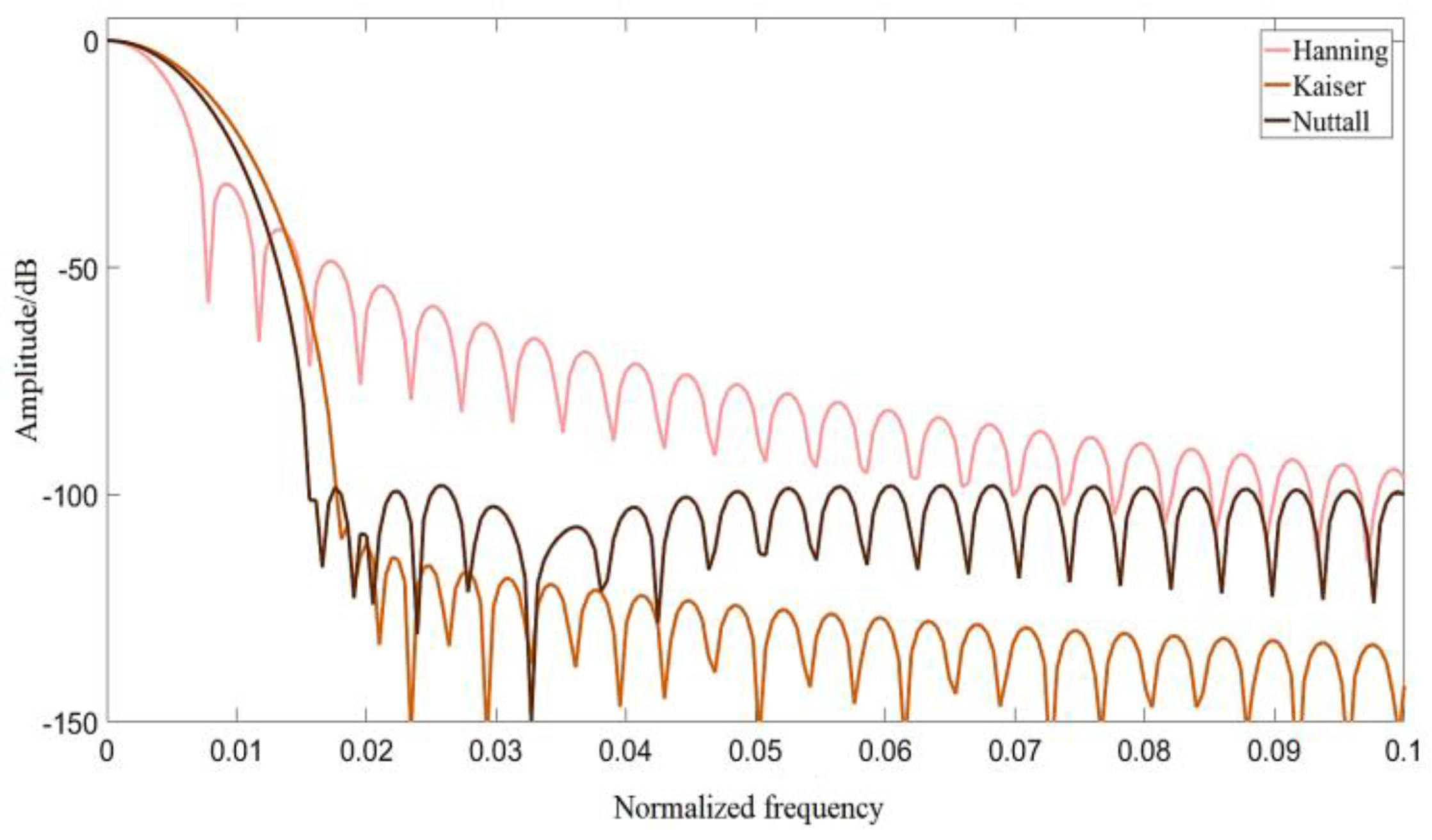
3.1. Comparison of Phase Calculation Errors
3.2. Spatial Localization Simulation
3.3. Finite Element Simulation Experiment
3.4. Analysis of Experimental Results
4. Conclusions
Author Contributions
Funding
Data Availability Statement
Conflicts of Interest
References
- Lu, S.-Y.; Sha, K.; Lu, C.-L. Application progress of computer navigation in trauma orthopedic surgery. J. Guangxi Med. Univ. 2022, 39, 849–855. [Google Scholar] [CrossRef]
- Song, M.; Chen, T.; Chen, C.; Chen, J. Analysis of Rectification Measures for Radiation Emission of Medical Optical Positioning System. J. Saf. Electromagn. Compat. 2022, 4, 67–70. [Google Scholar]
- Pei, D.; Huang, D.; Chen, J.; Zhang, J. Research status and development trend of surgical navigation system. Clin. Med. Eng. 2017, 24, 1326–1328. [Google Scholar]
- Hassfeld, S.; Mühling, J. Computer assisted oral and maxillofacial surgery—A review and an assessment of technology. Int. J. Oral Maxillofac. Surg. 2001, 30, 2–13. [Google Scholar] [CrossRef] [PubMed]
- Decker, R.S.; Shademan, A.; Opfermann, J.D.; Leonard, S.; Kim, P.C.; Krieger, A. Biocompatible near-infrared three-dimensional tracking system. IEEE Trans. Biomed. Eng. 2017, 64, 549–556. [Google Scholar] [PubMed]
- Bale, R.; Widmann, G. Navigated CT-guided interventions. Minim. Invasive Ther. Allied Technol. 2007, 16, 196–204. [Google Scholar] [CrossRef] [PubMed]
- Wang, S. Research on Three-Dimensional Positioning System in Surgical Navigation. Ph.D. Thesis, Central South University for Nationalities, Wuhan, China, 2012. [Google Scholar]
- Zhao, X. Research on Medical 3D Electromagnetic Positioning System. Master’s Thesis, Harbin Institute of Technology, Harbin, China, 2019. [Google Scholar] [CrossRef]
- Li, G.; Su, M.; Zhu, D. An improved LM algorithm in bundle adjustment. J. Xi’an Univ. Sci. Technol. 2022, 42, 152–159. [Google Scholar]
- Zhang, H.; Wu, T. Application of genetic algorithm in solving nonlinear equations. J. Zhaoqing Univ. 2002, 4, 16–19. [Google Scholar]
- Chen, S.; Xu, L.; Zhuang, H.; Zhu, W. A Laser Radar System for Measurement of Separation Processes in Spacecrafts. Missiles Space Launch Technol. 2019, 5, 122–126. [Google Scholar]
- Dong, C.; Zhao, Y.; Zhang, C.; Li, M. Phase-based laser ranging system based on FPGA. Foreign Electron. Meas. Technol. 2021, 40, 5. [Google Scholar]
- Xi, J. Design of Phase Laser Ranging Instrument and Analysis of Influencing Factors on Its Performance. Master’s Thesis, Xi’an University of Technology, Xi’an, China, 2022. [Google Scholar] [CrossRef]
- Chen, H. Research on Phase Laser Ranging System. Master’s Thesis, China Jiliang University, Hangzhou, China, 2019. [Google Scholar] [CrossRef]
- Nejad, S.M.; Fasihi, K.; Olyaee, S. Modified Phase-Shift Measurement Technique to Improve Laser-Range Finder Performance. J. Appl. Sci. 2008, 8, 316–321. [Google Scholar]
- Xu, S.; Chen, Y.; Zhao, Q. Research on implementation method of small size high-precision laser ranging system. Infrared Laser Eng. 2008, s3, 243–246. [Google Scholar]
- Poujouly, S.; Journet, B.; Miller, D. Laser range finder based on fully digital phase-shift measurement. In Proceedings of the 16th IEEE Instrumentation and Measurement Technology Conference, Venice, Italy, 24–26 May 1999; IMTC/99. IEEE: Piscataway, NJ, USA, 1999; Volume 3, pp. 1773–1776. [Google Scholar]
- Jia, F.; Ding, Z.; Yuan, F.; Ge, D. Laser dynamic target real-time ranging system based on all-phase fast Fourier transform spectral analysis. Acta Opt. Sin. 2010, 30, 2928–2934. [Google Scholar]
- Chen, Z.; Wang, L.; Wang, C.; Shen, P.; Li, Z. Power harmonic analysis method based on combined cosine optimization window four-spectrum line interpolation FFT. Power Syst. Technol. 2020, 44, 1105–1113. [Google Scholar] [CrossRef]
- Hao, Z.; Gu, W.; Chu, J.; Ma, C. A power network harmonic detection method based on the four-spectrum-line interpolation FFT. Power Syst. Prot. Control 2014, 42, 107–113. (In Chinese) [Google Scholar]
- Liu, Y. Key Technology Research on Phase Measurement Distance Based on RF Electro-Optic Modulation. Ph.D. Thesis, Huazhong University of Science and Technology, Wuhan, China, 2015. [Google Scholar]
- Li, Z. Research on Phase Discrimination Method for Phase-Based Laser Ranging. Master’s Thesis, Xidian University, Xi’an, China, 2014. [Google Scholar]
- Bai, Y. Research on Six Degrees of Freedom Electromagnetic Positioning Vector Signal Transceiver Technology. Master’s Thesis, Jilin University, Changchun, China, 2015. [Google Scholar]
- Chen, M. Research on Six Degrees of Freedom Electromagnetic Positioning Algorithm and Device Design. Master’s Thesis, Jilin University, Changchun, China, 2015. [Google Scholar]


| Parameter Requirements | High Frequency | Difference Frequency |
|---|---|---|
| sampling rate | ≥1.2 GHz | ≥40 KHz |
| signal-to-noise ratio | ≥30 dB | ≥30 dB |
| sampling accuracy | 24 bit | 24 bit |
| price | ≥¥800 | ¥150 |
| Algorithm | Hanning Window | Triangular Window | Hamming Window |
|---|---|---|---|
| A0 | −2.441 × 10⁻⁵ | −4.9663 × 10⁻⁴ | 3.55 × 10⁻⁴ |
| A1 | −1.922 × 10⁻⁴ | −1.772 × 10⁻⁴ | −2.554 × 10⁻⁴ |
| A3 | −3.48 × 10⁻⁵ | −1.4393 × 10⁻⁴ | −4.476 × 10⁻⁵ |
| f1 | 8.930 × 10⁻⁷ | 1.9157 × 10⁻⁵ | 1.166 × 10⁻⁵ |
| f3 | 2.669 × 10⁻⁶ | 5.2333 × 10⁻⁵ | 3.638 × 10⁻⁵ |
| −1.82 × 10⁻⁵ | −5.6136 × 10⁻⁵ | −1.948 × 10⁻⁴ | |
| −5.414 × 10⁻⁵ | −2.8074 × 10⁻⁴ | −2.599 × 10⁻⁴ |
| Algorithm | Zero-Crossing Detection Method | Maximum Value Detection Method | Moving Correlation Method |
|---|---|---|---|
| error | 1.3 × 10⁻³ | 2 × 10⁻⁴ | 3.9 × 10⁻³ |
| Algorithm | Rotation Matrix Method (Actual Data) | Quaternion Method (Actual Data) | Spectral Line Interpolation Method (Theoretical Simulation) |
|---|---|---|---|
| degrees of freedom | 6 | 6 | 3 |
| positioning error/mm | 22–23 | 8.5–25.9 | 2.3 |
| angle error/° | 10 | 7 | - |
Disclaimer/Publisher’s Note: The statements, opinions and data contained in all publications are solely those of the individual author(s) and contributor(s) and not of MDPI and/or the editor(s). MDPI and/or the editor(s) disclaim responsibility for any injury to people or property resulting from any ideas, methods, instructions or products referred to in the content. |
© 2023 by the authors. Licensee MDPI, Basel, Switzerland. This article is an open access article distributed under the terms and conditions of the Creative Commons Attribution (CC BY) license (https://creativecommons.org/licenses/by/4.0/).
Share and Cite
Jing, Z.; Gong, Y.; Cai, H.; Tang, H. Research on the Three-Dimensional Electromagnetic Positioning Method Based on Spectrum Line Interpolation. Electronics 2023, 12, 3988. https://doi.org/10.3390/electronics12193988
Jing Z, Gong Y, Cai H, Tang H. Research on the Three-Dimensional Electromagnetic Positioning Method Based on Spectrum Line Interpolation. Electronics. 2023; 12(19):3988. https://doi.org/10.3390/electronics12193988
Chicago/Turabian StyleJing, Zhixin, Yulin Gong, Hua Cai, and Haoxiang Tang. 2023. "Research on the Three-Dimensional Electromagnetic Positioning Method Based on Spectrum Line Interpolation" Electronics 12, no. 19: 3988. https://doi.org/10.3390/electronics12193988
APA StyleJing, Z., Gong, Y., Cai, H., & Tang, H. (2023). Research on the Three-Dimensional Electromagnetic Positioning Method Based on Spectrum Line Interpolation. Electronics, 12(19), 3988. https://doi.org/10.3390/electronics12193988