1. Introduction
The development of an accurate dynamic model is crucial for the purpose of optimization, control, fault diagnosis, and prognosis [
1,
2,
3]. There are three main modeling approaches for dynamic systems: the physics-based approach, data-driven approach, and hybrid approach. In the physics-based approach, the governing equations of a system are formulated from conservation laws, and they are solved analytically or numerically, while the data-driven approach uses a combination of data and deep learning techniques.
Machine learning (ML) techniques [
4], and its subset, that is deep learning (DL) methods [
5] such as Neural networks (NNs), have received significant attention in the field of science and engineering due to their capability in modeling nonlinear and complex systems [
6]. The modeling of a dynamic system using NNs or ML techniques can be implemented in two ways: purely data-driven or physics-informed data-driven implementation. The purely data-driven model, otherwise called a surrogate model, is developed by creating a neural network architecture that maps the input of a system to its output while the network parameters are optimized to ensure an accurate prediction. Examples of such neural networks are the multilayer perceptron (MLP) or FNN, CNN, recurrent neural network (RNN), and transformer. A recent ML technique that is used to discover parsimonious models of a system from data is called sparse identification of nonlinear dynamics (SINDy). This method has the advantage of interpretability and is subject to a tradeoff between structural complexity and the accuracy of the resulting models [
7,
8].
In the case of the hybrid modeling, a physics-informed neural network is a new form of NN that uses physical laws (or insights) described by ODEs or PDEs to guide the construction, training, and optimization of its underlying data-driven model [
9]. When training a PINN model, the physical laws provide constraints to the network, and the advantage of this is that the issue of overfitting is prevented, less training data are required, and the model becomes robust [
10,
11,
12].
Furthermore, there are different nonlinear phenomena in mechatronic systems and a data-driven or hybrid model can handle such complex characteristics. Friction is the most common one, and it usually affects the dynamics and overall efficiency of any system. When modeling a mechatronic system through the physics-based approach, frictional losses are integrated into the model equation to improve the model’s accuracy. The problem with this is that there is no general model for capturing frictional losses and friction models (whether static or dynamic) [
13,
14] introduce more unknown parameters to the model equations. Thus, it is advantageous to use a purely data-driven or hybrid approach in identifying friction [
15].
This review investigates various data-driven modeling methods employed for identifying mechanical and electronic systems with a real-world classic system. There are many data-driven methods that have been proposed in the literature; however, the scope of this work is limited to these machine learning methods: FNN, CNN, LSTM, transformer, SINDy and PINN. Other promising data-driven methods such as symbolic regression [
16,
17], dynamic mode decomposition [
18,
19], and new variants of neural networks like Fourier neural networks [
20] are not covered. The contributions of this work are as follows:
Four distinct purely data-driven models were developed for a geared DC motor, namely, FNN, CNN, LSTM, and transformer models. These models demonstrated high prediction accuracies. In addition, SINDy approach was employed to directly discover various parsimonious models of the system from experimental data. Using different optimizers, three sparse regression models were generated, utilizing a library of candidate functions with a polynomial order of 2;
PINN modelling method was employed to resolve coupled first-order differential equations governing a geared DC motor. The unidentified physical parameters of the dynamical system were successfully determined. The results demonstrate that the PINN approach effectively forecasts the dynamic response of the nonlinear system and estimates the unmeasured system state, specifically the armature current.
Our findings clearly demonstrate the satisfactory predictive capabilities of six distinct ML models. Additionally, we shed light on their strengths and weaknesses, including factors like interpretability and computational complexity, through a practical case study.
The paper’s structure is depicted in a mind map in
Figure 1.
Section 2 covers essential background concepts, such as system identification, forward and inverse modeling problems, online and offline parameter identification, and dynamic modeling with friction. In
Section 3, we discuss the utilization of neural networks and machine learning techniques for the dynamic modeling of mechatronic systems. Additionally,
Section 4 presents a case study on the dynamic modeling of a geared DC motor, employing various data-driven and hybrid approaches, along with their potential applications. Finally, in
Section 5, the paper summarizes the research contributions and identifies gaps for future studies.
The results presented in this paper can be reproduced through the code available on GitHub [
21].
2. Background
In order to provide a proper context to our work, the following key concepts of modeling are presented in this section: system identification, forward and inverse problems, online and offline parameter identification, and dynamic modeling with friction.
2.1. System Identification
System identification, as the name suggests, is the process of identifying a system behavior by means of its measured or observed input and output data [
22]. Through different algorithms that are based on numerical optimization, the relationship between the system input and output is mapped during identification [
1].
As illustrated in
Figure 2, system identification involves four main steps: data collection or acquisition, model structure definition or selection, model parameters estimation, and model validation [
2,
23]. The first step involves getting input–output data from the physical system by designing and conducting an experiment covering the system’s operating limits/bounds. It is crucial to acknowledge that the obtained dataset could have outliers and this necessitates data prepossessing operations such as normalization, resampling, or filtering. Secondly, a model structure such as transfer function, state-space, autoregressive with exogenous (ARX), or neural network is selected depending on the available insight or prior knowledge of the system under consideration. In the third step, the model parameters are trained or estimated using different algorithms like LS or backpropagation. During estimation, the model parameters act as a driver and play the role of driving the model, thereby fitting its response to match that of the actual system. The fourth and last step is to validate the estimated model. This is performed to guarantee that the developed model will serve the intended application (e.g., control or fault detection). In a scenario where the developed model turns out to be unsatisfactory, the identification process is reworked (i.e., performed all over again) [
2,
4]. For this reason, system identification is regarded as an iterative process and it involves the user trying out different choices in terms of the model structure and even the estimation algorithm to arrive at the best model.
There are three main modeling approaches: physics-based, data-driven, and hybrid modeling.
Physics-based modeling: This method utilizes knowledge of the underlying physical laws governing the system’s behavior. The equations and parameters are theoretically determined and solved [
1]. However, in reality, a purely physics-based model is impractical for large-scale or complex systems [
24,
25]. The model developed through this approach is referred to as a mathematical one;
Data-driven modeling: This method is suitable for complex nonlinear systems where little or no knowledge of their governing physical laws exists. The model structure and parameters are unknown, and the model architecture is not based on physical laws. As a result, the parameters often lack physical meaning or interpretation [
1,
26]. The model developed through this approach is known as data-driven or intelligent;
Hybrid modeling: In this case, partial knowledge about the system is available. The model structure is either fully or partially known, and its parameters are estimated using system data [
1,
27]. The resulting model is called hybrid or physics-informed data-driven.
The three modeling approaches are depicted in
Figure 3. The upper arrow indicates increasing complexity, while the lower arrow indicates the direction of increasing knowledge and model assumptions according to the modeling methods.
Remark 1. Based on their level of transparency and ease of understanding, the modeling approaches are classified as follows: (i) white-box modeling, which relies on physics-based principles; (ii) black-box modeling, which is data-driven in nature, (iii) grey-box modeling, which combines physics-based and data-driven aspects [1]. 2.2. Forward and Inverse Modeling Problems
The modeling problems posed by dynamical systems can be classified into forward and inverse problems. The forward modeling problem involves computing a system response or solution given its mathematical model and parameters [
28]. In forward problems, ordinary differential and partial differential equations (ODEs and PDEs) are solved analytically or numerically using the Euler method, Runge–Kutta method, finite element method, finite difference method, and so on. In contrast, the inverse modeling problem involves the estimation of unknown model parameters that would give a small prediction error when compared to the output data observed from a physical system [
29]. The parameters can be identified (estimated) using various algorithms such as least squares (LS) [
30], recursive least squares (RLS) [
31], the genetic algorithm (GA) [
32], NNs [
33], etc.
2.3. Online and Offline Parameter Identification
The concept of identifying the model parameters of a system is known as parameter identification, and this topic can be viewed as an inverse modeling problem. Parameter identification is performed either online or offline. In online parameter identification, model parameters are estimated in real time with the help of algorithms such as RLS [
30,
34] and the extended Kalman filter [
35,
36], as new sensor data are available from the physical system. On the other hand, offline parameter identification is conducted by acquiring input–output data from the system, storing the data, and then using an algorithm like LS or GA to estimate the unique parameters of the system. In
Table 1, the two-parameter identification methods are compared in terms of the type of parametric results they give, the ease of data preprocessing, and the computational power and storage demands.
2.4. Dynamic Modeling with Friction
In mechatronic systems, such as pendulums, DC motors, and mass-damper setups, modeling can be accomplished using either first principles or physical laws. However, achieving accurate models often requires identifying the system’s parameters. One major challenge is accurately representing the impact of friction, a nonlinear phenomenon that affects the efficiency of these systems [
37,
38].
Friction models can be categorized into static and dynamic models. Static models assume no relative motion during standstill (resting friction phase) and describe the relationship between friction force and relative velocity. On the other hand, dynamic models capture the features of presliding and sliding regions, including their transition effects [
39].
Static models consist of Coulomb friction, viscous friction, the Stribeck effect, Karnopp, and Armstrong. Moreover, dynamic models include Dahl, LuGre, Leuven, and bristle friction models [
40,
41,
42,
43].
Applying an accurate friction model can facilitate friction compensation, helping to prevent issues such as slow responses, tracking errors, stick-slip motion, and limit cycles [
44,
45]. Notably, for dynamic systems developed purely through data-driven approaches, a separate friction model is unnecessary, as frictional losses are already accounted for in the experimental data used to build the model.
3. Dynamic Modeling of Mechanical and Electronic Systems Using Neural Networks and Machine Learning Techniques
Artificial neural networks (ANNs) or simply NNs are deep learning techniques (which is a subset of machine learning) inspired by the functioning of neurons in the brain. There are three fundamental learning approaches used in machine learning: they include supervised, unsupervised, and reinforcement learning [
46]. Neural networks predominantly depend on supervised learning, utilizing labeled data for predictive tasks. In contrast, unsupervised learning reveals patterns in unlabeled data, while reinforcement learning centers on trial-and-error decision-making processes.
An NN can learn complex functions by extracting relations from training data; thus, it is regarded as a universal approximator. NNs can be used in developing data-driven models for nonlinear, multivariable, and complex dynamics. A typical NN consists of interconnected neurons with weights and a bias. In addition, an activation function is also used in a neuron to filter the information that is transferred to the next neuron. Some common activation functions are the rectified linear unit (ReLU), sigmoid, hyperbolic tangent function (Tanh), and pure linear function [
47,
48]. The algebraic calculation that happens within a single neuron is:
where
is the output of the neuron after activation,
z denotes the output of the neuron after passing the summation unit,
represents the activation function,
is the weight associated with the
i-th input,
b is the bias, and
n is for the number of input (
x).
The model of a single neuron is depicted in
Figure 4, see [
49].
Through supervised training, a learning algorithm is used to iteratively adjust the network parameters based on the error between the predicted output and the training data outputs. The error is computed during a forward pass while the weights are optimized from the output layer to all the other layers during the backward pass (this is called error backpropagation) [
50]. Most NN models use the gradient-based method to minimize the loss
J of the network, i.e.,
where
J is the loss between the target output and predicted network output,
y the target output,
is the predicted output by the network, and
m represents the number of data points. Accordingly, the weights and bias being the trainable parameters of the neuron are updated as iteratively as follows:
where
is defined as the learning rate.
The manner in which gradient descent optimizes the weight parameter
w is illustrated in
Figure 5.
Besides gradient descent, other common training algorithms are adaptive gradient descent, momentum, adaptive momentum, Newton, quasi-Newton, and Levenberg–Marquart.
In this section, different types of NN structures, such as MLP, CNN, RNN and PINN, including ML methods such as SINDy will be discussed. Moreover, we will compare those models based on their advantages, disadvantages, and applications.
3.1. Multilayer Perceptron Network
An MLP or FNN has three layers: the input layer, hidden layers, and output layer. The MLP network illustrated in
Figure 6 consists of an input, three hidden layers, and an output layer. It is possible to improve the fit of a network by using more layers; however, this can also increase the training time. The size of neurons in the hidden layer can cause a poor fit (underfitting), while many neurons can result in overfitting (a poor generalization of the network to new data). A middle way is usually sought through trial and error for a good result [
50].
A nonlinear autoregressive with exogenous inputs (NARX) model is commonly used in the data-driven modeling of dynamic systems. The structure of a NARX model is
where
is the predicted output at a future time
,
f is a nonlinear function, and
is the regressor vector of the form
where
and
are time delays, and they are determined based on the system order.
An FNN can be employed for estimating the nonlinear function of the NARX model structure. In the specific case study [
4] presented, a NARX-based neural network was utilized to develop a data-driven model for a DC motor. This neural network mapped the nonlinear relationship between the motor’s PWM signal and its speed. Similarly, in another study [
51], an NN was used to model a brushless DC motor. The NN was trained with experimental data comprising torque, angular velocity, and motor efficiency. The dataset was split into training (85%), testing (10%), and validation (5%) datasets. The trained model took torque and angular velocity as inputs and provided motor efficiency as the output. Post-training, the NN model demonstrated good performance, with a resulting mean square error of 1.5.
3.2. Convolutional Neural Network
A convolutional neural network is popularly used in the field of computer vision for classification tasks, but it is also useful for regression tasks [
52]. The convolutional layer is the central part of a CNN architecture and
Figure 7 shows a one-dimensional CNN architecture. Suppose we are given an
time-series input data. The data are first transformed to a three-dimensional array by data sequencing using
g number of data points as the sliding window. During the convolution process, a set of weights known as kernels or filters slide through the transformed input data. The dot product of the kernel weights and the input local receptive field is computed, they are summed, a bias is added, and each element of the resulting array is passed through a nonlinear activation function [
52,
53].
Mathematically, convolution operation is expressed as:
where
and
are the output and input of the convolution, the convolution operator is denoted by ∗,
i is the iteration index, which is determined by the input (
) size,
represents the kernel or filter of the
j-th neuron in layer
l,
K is the kernel size, and
is a scaler bias of layer
l.
The convolution output
is passed through an activation function (such as ReLU) and the final output of the layer is:
The outputs of the convolutional layer
, which are called feature maps, are flattened to a feature vector at the fully connected layer. The other layers that are used in a CNN architecture for classification purposes include the pooling layer and dropout layer, which are used to reduce the computation size of the model and help to prevent overfitting. A dense layer can also be used after the fully connected layer, particularly when dealing with a regression problem [
10,
53].
A CNN was used in [
54] to identify the model of a nonlinear system. The Weiner–Hammerstein system was used to form the dataset and the performance of a CNN and MLP in system identification was compared. The simulation result showed that the CNN performs better than MLP when a noisy data are used.
3.3. Recurrent Neural Network
An RNN is a type of NN that is suited for modeling time-series or sequential data. The reason is that RNN, unlike MLP, uses the concept of memory, allowing the network to store the state of the previous step or useful information from past inputs, and that information is used when generating the output of the next sequence [
52]. An RNN architecture is shown in
Figure 8.
It is worth noting that the same weights and biases are used in the network as it unfolds at each time step
t. At time
t, the network input is
, the state is
, the output is
, and particularly:
where
,
, and
are the weights associated to the input, state, and output, respectively;
and
are the state and output biases.
An RNN uses backpropagation through the time (BPTT) algorithm to update its weight and minimize the total error of the network [
55].
The partial derivatives/gradient of the network with respect to the weights can be mathematically calculated as follows:
However, due to the huge multiplication involved when the partial derivative of the error is calculated across the hidden states, the gradient may end up exploding or vanishing.
There are different RNN architectures that are used to solve various ML problems. They are bidirectional recurrent neural networks, gated recurrent units, or even LSTM [
56].
3.4. Long Short-Term Memory
This is a special type of RNN that can handle long-term dependencies in data and can also eliminate the vanishing gradient problem of an RNN. An LSTM cell depicted in
Figure 9 stands for a computational unit that controls the flow of information. The key parts of an LSTM unit are the cell state, forget gate, input gate, and output gate. The operations performed in an LSTM unit to process information are as follows:
Forgetting the irrelevant part of the previous state;
Storing the most relevant new information;
Updating the internal cell state;
where
and · represents element-wise multiplication.
Generating an output;
where
.
When training the LSTM network, the weights and biases of the input, output, and forget gates are updated at each time step through the BPTT algorithm [
52,
55].
The LSTM network was used to model the rolling friction of a mechanical system in [
57] to capture the system’s friction characteristics at the presliding region. The authors proposed an initial value design for the RNN such that the final value of the last training set is used as the initial value of the next training. The effectiveness of the developed model was verified with the LuGre and Kiozumi models using an experimental setup consisting of a motor, gear, load, encoder, and a clamp to adjust the friction level.
3.5. Transformer Network
Transformers, well-known for their sequence generation capabilities, have garnered significant attention in the domain of natural language processing due to their impressive performance in generative tasks. Their success can be attributed to the attention mechanism, which enables the learning of long-term dependencies in data without the need for recurrent connections, such as RNN and LSTM [
58]. Furthermore, transformers offer the advantage of supporting parallel processing of input sequences, unlike LSTM, which requires sequential processing. This feature makes transformers highly efficient for training, especially when dealing with extensive datasets.
The encoder part of the transformer network illustrated in
Figure 10 can be used in time-series prediction, fault classification, anomaly detection, etc. [
59,
60].
The steps involved in time series-based modeling using transformer encoder networks are as follows:
Data preparation into sequence. Time series data acquired experimentally from a mechatronic system are intrinsically ordered, thus negating the need for position encoding;
The sequence is inputted to a transformer encoder, which comprises
N multihead attention and feedforward layers [
59,
60,
61]. The multihead attention enables the model to understand both long- and short-term dependencies or relationships among various time steps in the sequence. Moreover, the feedforward layer is responsible for capturing high-level and complex interactions and patterns in the data.
where
,
, and
are the weight matrices of the
i-th attention head,
represents the weight matrix of the multihead attention,
h represents the total number of heads, and concat is a function for concatenating the outputs of the attention heads.
The equation below describes the attention mechanism used in the network:
In this equation, , , and represent the query, key, and value matrices, respectively. These matrices are obtained by multiplying the input feature matrix X with the parameter matrices , , and . Here, ’d’ denotes the dimension of Q, K, and V.
The feedforward layer processes the output of the multihead attention layer. It consists of a fully connected layer (e.g., MLP or 1D CNN can be used), followed by a ReLU or Gaussian error linear unit (GeLU) activation function, and a dropout layer;
The output layer involves a fully connected layer along with a linear activation function;
Training and optimization: The transformer encoder undergoes training with input sequences, and the corresponding system output serves as the target. The model is then optimized through a fitting loss function like MSE (refer to Equation (
3)) to minimize the discrepancy between predicted and actual values;
Model evaluation: after being trained, the transformer encoder can be utilized for inference, enabling predictions to be made using novel sequences of dynamic system data.
Though transformer network is a state-of-the-art algorithm but its application in the dynamic modeling of systems is limited as reported in [
62].
3.6. Physics-Informed Neural Networks
The physics-based modeling method is easily affected by a high bias arising from simplifying assumptions. Similarly, the solely data-driven approach exhibits a high variance when the experimental data fails to encompass the system’s entire operating range. To address these respective issues of bias and variance in physics-based and purely data-driven modeling, a novel data-driven modeling technique based on physics-informed neural networks (PINN) can be employed.
Recently, there has been a growing interest in the application of PINNs in science and engineering. PINNs effectively combine data and physical laws to address supervised learning tasks. This novel approach finds utility in solving forward problem-solving tasks involving ODEs and PDEs. Additionally, PINNs demonstrate proficiency in handling inverse problems, such as parameter identification in differential equations. The implementation of the algorithm delivers the continuous and discrete PINN approach. In the continuous one, the system equation is integrated into the neural network architecture’s loss function.
Consider solving the following ordinary differential equation:
where
u represents the dependent variable,
t is the independent variable (time), and
is a system parameter.
In the continuous PINN approach, we approximate the solution to Equation (
19) using a neural network
such that
, with
.
By computing the derivatives of the network output with respect to its inputs using automatic differentiation [
63], we can calculate the equation’s residual in the form:
This motivates the loss function to optimize the neural network:
The model’s training objective is to minimize
by adjusting the weights (
w) and biases (
b) of the network
. The physics loss ensures that the system’s governing equations are enforced. Various case studies and engineering problems where this approach has been applied can be found in [
10,
12,
63,
64,
65,
66,
67,
68]. Additionally,
Figure 11 illustrates a continuous PINN architecture demonstrating the physics-guided loss formulation.
The discrete approach or multistep PINN involves utilizing multistep discretization techniques such as forward Euler and other Runge–Kutta schemes to numerically discretize the system equation over time. The unknown functions or state update vector are approximated using neural networks.
To solve the first-order Equation (
19) numerically, two methods can be employed. The first one is the forward Euler method, expressed as:
where
f represents a function dependent on
t and
u itself. Alternatively, the same equation can be solved using the Runge–Kutta 4th order method:
where
and
is the step size.
The functions present in both discretization schemes are replaced with neural networks and the networks are trained using the regular loss of typical neural networks (i.e., the MSE between the actual
u and predicted
at each time step). This approach was discussed in following papers [
69,
70,
71] and used to model the nonconservative forces in the dynamic equation of an inverted pendulum in [
11]. PINNs are usually implemented with feed-forward neural networks because they are faster to train. However, this does not rule out the possibility of using other NNs. For instance, a physics-informed ML approach was investigated in a recent study for modeling the surface roughness of a milling process [
72].
3.7. Sparse Identification of Nonlinear Dynamics
SINDy is a promising ML technique that can be used for the discovery of a system’s governing equations directly from data. This technique was introduced in [
7], and it can be used to discover ordinary and partial differential equations. Suppose we consider a nonlinear dynamical system with the form:
where
represents the state of the system,
u is the control input, and
f denotes the vector field of the system.
The SINDy algorithm is implemented in the following steps to find the parsimonious model that will describe the system by employing sparse regression.
Collect the time-series data of the dynamical system,
X, and
U and compute the derivative of system states,
. If
x comprises
m states, then
and:
where
are the sampling points of the time-series data;
Create a library candidate function that consists of constant, polynomial of degree
k (which is user defined) and the trigonometric terms:
Solve a sparse regression problem:
where the matrix
consists of sparse vectors that are matched to their corresponding active terms in the candidate function library
.
To find
, a sparse optimization is conducted to minimize the following function:
There are different methods of solving the optimization problem. They include least absolute shrinkage and selection operator (LASSO) [
73], stepwise sparse regression (SSR) [
74], sequential threshold least-squares (STLSQ) [
7,
75], and sparse relaxed regularized regression (SR3) [
76,
77].
In [
78], the SINDy algorithm was used to model the discrepancies between the observed data and the simplified mathematical models of some physical systems. Specifically, the algorithm was used to discover the discrepancies induced by parameter inaccuracy or model insufficiency. The examples considered to demonstrate the algorithm’s effectiveness include the Van der Pol oscillator and a double inverted pendulum on an actuated cart.
3.8. Comparison of Different ML Methods
Table 2 shows the pros, cons, and application domain of each of the ML models discussed in the previous subsections.
4. Identification of a Direct Current Geared Motor’s Model—Real Application
In this mechatronic study, we undertook an analysis focused on the dynamic model of a geared DC motor. Our methodology encompassed three distinct approaches: a physics-based approach, a purely data-driven approach utilizing various neural network models (FNN, CNN, LSTM, and SINDy), and a hybrid approach known as PINN.
The governing equations of the physical object under examination are derived from the mechanical and electrical components’ operational concepts, utilizing Newton’s second law and Kirchhoff’s laws, respectively [
79,
80]. These fundamental principles lay the foundation for the mathematical system model detailed in
Section 4.1.
In parallel, the purely data-driven models were directly developed from experimental data. To achieve this, two datasets were acquired, comprising input and output data from a geared 12V DC Motor (SG555123000-10K). These datasets encompass the full operating range of the motor and were designated as the training and test datasets.
The data acquisition’s control structure is depicted by the block diagram in
Figure 12. This diagram provides an insightful view of the experimental setup’s configuration.
An open-loop control experiment was conducted utilizing a time-varying PWM step signal as the input to the physical system, with the motor’s angular speed or rotational velocity as the measured output, which was obtained through an encoder.
To execute the experiment, the necessary hardware and specifications can be sourced from [
81]. Subsequently, the collected data were employed to train four neural network models and a machine learning model, elaborated in
Section 4.2 and
Section 4.3. Furthermore, the same dataset and the system’s physical laws were leveraged to formulate a PINN model in
Section 4.4. The training and testing csv files are accessible at [
21].
4.1. Physics-Based Model of the Motor
A geared DC motor possessing uncertain frictional resistance forces can be classified as a nonlinear system, showcasing common nonlinear phenomena such as dead zones and backlash [
82]. However, to facilitate a simplistic and approximate physical representation, the system is conventionally characterized as a second-order linear system. The system’s diagrammatic representation can be observed in
Figure 13.
The equation of the electrical circuit shown on the left-hand side of the schematic is:
where
;
V and
i are the armature voltage [V] and current [A], respectively;
L and
R are the armature inductance [H] and resistance [
], respectively, and
is the back EMF constant [V·s/rad]; and
is the angular position of the rotor shaft [rad].
The total motor torque
[N·m] produced by the motor is proportional to
i, i.e.,
where
and
are the torques applied to the shaft of the rotor and gear [N·m]. Comparing Equations (
31) and (
32), we find:
where
and
are the shaft inertia of the rotor and gear [kg·m
2];
and
are the damping coefficient of the rotor and gear [N·s/m], respectively;
is the motor torque constant [N·m/A];
is the gear ratio [-]; and
is the shaft position [rad].
Let
,
,
, and
, then Equations (
31) and (
33) can be rewritten as two first-order coupled differential equations of the form:
When the physical parameters mentioned in Equations (
34) can be determined, it becomes feasible to estimate the system’s dynamic response numerically. However, a challenge arises when dealing with the unknown parameters of the DC motor, requiring careful estimation. Therefore, the focus is now on investigating the capability of utilizing the PINN modeling paradigm to unveil the motor parameters. This means the creation of a physics-guided data-driven model is explored in
Section 4.4.
4.2. The FNN, CNN, LSTM, and Transformer Networks Estimating Models of the Motor
Now, we investigate four neural networks: FNN, CNN, LSTM, and the transformer, which are used to estimate the purely data-driven models of the system. The models were trained differently using 20 epochs for each model and their structures are shown in
Table 3.
It is also evident that, despite the noise in the acquired angular speed data from the physical system, the time history in
Figure 14 depicts a close match between the model predictions and the actual system output, that is, the angular speed of the geared DC motor.
In this study, we used the Adam optimizer with a learning rate of 0.001 for training each model. The computation times are shown in
Table 2. The FNN model trained faster than the CNN, LSTM, and transformer models. The transformer network performed well in terms of validation loss but required more time to train due to its complex attention mechanisms and limited dataset size. The problem’s complexity contributed to the time-consuming training process. For reproducing the results, the numerical code is available in the specified repository [
21].
All four models had similar prediction errors or validation loss, indicating only slight differences in their performance. Improving the models’ accuracy would involve exploring various network hyperparameters, such as the number of layers, neurons, optimizer type, learning rate, and training epochs. To enhance the transformer model’s performance, incorporating position encoding to capture the input data’s sequential nature explicitly would likely lead to significant improvements in predictions.
Remark 2. The models were trained offline using TensorFlow deep learning framework on a computer equipped with an Intel Core i7 1.80 GHz CPU, 16-GB RAM, and a NVIDIA GeForce MX150 4 GB GPU.
4.3. SINDy Model of the Motor
SINDy, a machine learning method, was utilized to reveal the system’s dynamic equations following the approach detailed in
Section 3.7. This process involved employing the pySINDy framework introduced in [
83], which allows the customization of the library candidate function and the optimizer selection, along with the option to choose a differentiation method. For numerical differentiation, the finite difference method was used. The library candidate function for representing the sparse system incorporated the geared DC motor’s speed and voltage data, utilizing a third-order polynomial as the set order.
The discovered dynamical models of the system with SSR optimizer are as follows:
with the LASSO optimizer:
and with the FROLS optimizer:
As shown in
Figure 15, the simulation responses of the three models indicate that SINDy is effective in identifying a nonlinear system from experimental data.
The computation times for the SINDy models are shown in
Table 4.
The discovered model suggests a library candidate function with a polynomial of order 2 being sufficient to represent the dynamics of the system. The numerical code that was used to generate the reported results is available at the repository [
21].
4.4. PINN Model of the Motor
Deep FNNs have been used in several studies to implement the PINN modeling approach because they are computationally efficient [
63,
69,
84,
85]. Hence, this work examines the use of a three-layer-deep FNN with 32 neurons in each layer in implementing the PINN architecture. The PINN algorithm is described in
Appendix A and it was used in solving both direct and inverse problems.
The initial steps of the algorithm involve importing necessary packages (numpy, pandas, matlplotlib, keras, and tensorflow), initializing the system parameters, and loading training and testing datasets. Next, three feedforward neural network models with three hidden layers and 32 hidden neurons each are created. These networks use as the activation function, have two inputs, and produce one output. The weights and biases of these neural networks are randomly initialized and then trained.
The three neural networks, denoted as
,
, and
, represent the approximated solutions
,
, and
I corresponding to Equation (
34). During the training, the unknown physics parameters
,
,
,
,
,
L,
R, and
, along with the weights and biases of the networks, are initialized to enable the first prediction for each network error computation. This prediction is done in the forward pass, where three losses are computed with the approximated solutions
,
, and
: loss 1 is based on the mean squared error (MSE) from the first Equation (
34); loss 2 is based on the MSE from the second Equation (
34); and loss 3 is based on the MSE of the output shaft speed.
The physical parameters, and the weights and biases of each network, are updated during the backward pass using a standard backpropagation algorithm. The derivative of the total error with respect to the weights and biases of is computed using the sum of loss 1 and loss 3. Similarly, the derivative of the total error with respect to the weights and biases of is computed using loss 2. The Adam optimizer is used with a learning rate of 0.001 and the algorithm is trained for 20,000 epochs.
After training, the identified physics parameters are displayed, and the weights and biases are saved for future use. Additionally, the network predictions are plotted using the test dataset.
As shown in
Figure 16a,b, the PINN model successfully predicted the motor’s shaft speed and armature current even with limited training data containing noisy time-series of rotational velocity.
The system’s physical parameters, including the viscous friction coefficient, were estimated during training, and the resulting values are displayed in
Table 5. It is essential to acknowledge that the physical parameters obtained through the PINN algorithm are not unique. However, we constrained the search space for each parameter between 0.001 and 10 to determine their values.
The computation time for the PINN algorithm was 576.26 s, and the training loss was 6.57. For verification, the numerical code is available at the repository [
21].
4.5. Discussion of Results
The performance of the developed models can be compared based on the prediction error or residual of each model as shown in
Figure 17, while
Table 6 shows the performance of the models with metrics like mean absolute error (MAE), MSE, and root mean squared error (RMSE).
The plot depicts high prediction errors of the PINN model at the first three steady speeds of the DC motor. However, all models exhibit the least prediction error when the motor operates at speeds greater than 200 rpm. This high error at low speed is attributed to the motor’s significant nonlinearities, such as friction and noise. Additionally, based on the performance metrics of the six (6) ML models in
Table 6, the SINDy models (trained with different optimizers) gave the least errors, followed by the PINN and transformer models.
Despite this, all models, as shown in
Figure 14,
Figure 15 and
Figure 16, provide predictions close to the actual time-series motor output. They demonstrate good generalization with the new dataset. Furthermore, the developed SINDy models are computationally efficient compared to other methods. Although the PINN model requires a longer training time, it performs fast predictions once trained.
Moreover, the four data-driven models (FNN, CNN, LSTM, and transformer) lack interpretability, operating as black-boxes. In contrast, the SINDy and PINN models are explainable. In the case of the SINDy model, the constants and chosen candidate functions post optimization are sparse and known, while for the PINN model, the physics-based parameters that guide its adherence to physical consistency during training are identifiable. Specifically, the PINN model leverages the governing laws of the DC motor, enabling the identification of physical parameters, such as the friction coefficient. Additionally, the PINN architecture facilitates the estimation of unmeasured system states, like the armature current, a capability absent in other models. Despite the highlighted benefits of using PINN for dynamic system modeling, its applicability may be constrained when the bounds of physical parameters and governing equations remain unknown.
4.6. Potential Applications of the Developed Dynamic Models
4.6.1. Control
A dynamic model plays a vital role in the model-based design of classic controllers. It also helps simulate the designed controllers to validate their effectiveness in achieving the desired objectives set by the designer. These objectives typically involve stabilization, reference tracking, and disturbance rejection during the development of controllers.
For example, when dealing with an inverted pendulum, control objectives include stabilizing the pendulum in an upright position and rejecting external disturbances like wind. On the other hand, for a DC motor, the objective is to achieve reference speed tracking even at the presence of nonsmooth effects like stick-slip friction. Commonly employed control techniques for dynamic systems encompass the PID [
86], fractional order PID [
87], LQR [
88], fuzzy [
89], sliding mode [
90], and model predictive control [
81].
Additionally, in mechanical systems where friction significantly impacts performance, friction models are developed and utilized for friction compensation. However, friction models are needed for systems developed through the hybrid approach and systems built to study the effects of friction. This suggests that pure data-driven models incorporate frictional effects in their internal structure.
4.6.2. Fault Detection
Dynamic models play a crucial role in identifying potential faults within a system. This involves creating models for the system under normal operating conditions and various fault scenarios [
1]. By comparing the outputs of these models with the actual system’s responses, specific types of faults, such as actuator, sensor, or plant faults, can be detected [
91]. An inference system is employed for error classification. The accuracy of the fault models and distinct error characterization associated with each fault greatly influence the effectiveness of the fault detection algorithm.
4.6.3. Digital Twin
A digital twin is an updated online model of a system, incorporating either a physics-based or data-driven model. It utilizes real-time data from the actual system for continuous updates [
92]. Due to the extensive use of cloud computing and the Internet-of-Things, various industries employ digital twin technology for tasks like simulation, remote monitoring, control, predictive maintenance, and estimating the remaining useful life of physical assets or machines, thereby enhancing their reliability and safety [
93].
5. Conclusions
In this review paper, various modeling approaches were presented and relevant concepts were briefly discussed. These concepts encompassed forward and inverse modeling problems, online and offline parameter identification, and dynamic modeling with friction. The shift from physics-based to data-driven and hybrid approaches was investigated, and it was attributed to the challenges faced by physics-based models when dealing with highly complex systems. Formulating models based on physical laws or first principles becomes difficult in such cases. On the other hand, data-driven models lack interpretability, impeding their adoption by industrial experts who prefer models grounded in physical principles rather than black-box models. The potential of hybrid or physics-informed models to address complex systems while incorporating some level of physics was emphasized, thus providing applicability.
A real experimental station was presented to develop a model for a geared direct current motor using various modeling techniques. Four data-driven models (FNN, CNN, LSTM, and transformer) were constructed, along with the use of SINDy (a machine learning technique) to infer the system’s governing equations. Additionally, a physics-based model was employed to create a PINN model, which successfully identified the system’s physics parameters, such as the viscous friction coefficient, and predicted the armature current (not directly measurable during experimentation). The neural network models and machine learning techniques produced satisfactory results, but the SINDy and PINN models were considered superior in terms of their interpretability.
Three key applications of dynamic models were discussed: control, fault detection, and digital twin. However, there are still various open research areas in the modeling of mechatronic systems that require further exploration.
The recommendations for future work include enhancing the integration of physical laws into neural networks, especially for multibody mechatronic systems with dry friction. Utilizing physics-guided networks like physics-guided transformers would result in the creation of models that are transparent and can be easily explained. It is also suggested to explore improved versions of SINDy, such as SINDy with sensitivity analysis, to create interpretable and generalizable models for mechatronic systems. This should involve accurate, low-dimensional, and sparse machine learning models, considering noisy data. Moreover, the scarcity of experimental studies on the application of PINNs and SINDy for parameter identification and the modeling of mechatronic systems was noted. Therefore, extending the use of these techniques to different systems with more complexities (such as industrial manipulators or induction motors) and comparing their performance is proposed.
Author Contributions
Conceptualization, S.A. and P.O.; methodology, S.A. and P.O.; software, S.A.; validation, S.A.; formal analysis, S.A. and P.O.; investigation, S.A. and P.O.; resources, S.A.; data curation, S.A.; writing—original draft preparation, S.A. and P.O.; writing—review and editing, S.A. and P.O.; visualization, S.A. and P.O.; supervision, S.A. and P.O.; project administration, S.A.; funding acquisition, S.A. and P.O. All authors have read and agreed to the published version of the manuscript.
Funding
This research received no external funding.
Institutional Review Board Statement
Not applicable.
Informed Consent Statement
Not applicable.
Data Availability Statement
The data are available at the GitHub repository in [
21].
Acknowledgments
The authors would like to acknowledge the support of Lodz University of Technology and University of Huddersfield in making this research collaboration possible.
Conflicts of Interest
The authors declare no conflict of interest.
Appendix A
| Algorithm A1 The PINN algorithm. |
- 1:
Import: numpy, pandas, matplotlib, keras and tensorflow - 2:
Initialize the known system parameter, - 3:
Load the training and test dataset: acquired experimental data - 4:
Create three neural networks () Define: input and output dimensions, number of hidden layers and neurons Add as constrained weights or trainable parameters to Add as constrained weights or trainable parameters to - 5:
Initialize the weights and biases of - 6:
for to do - 7:
Get the predicted training dataset , , - 8:
Compute the derivative of the three networks: - 9:
Compute the system residuals (physics losses) with the losses due to prediction , - 10:
Compute the losses’ gradient and with respect to all the network parameters - 11:
Update network parameters (the weights and biases) of - 12:
Sum the losses of the two networks, - 13:
Print epoch g and the total loss of the system including the values of parameters - 14:
end for - 15:
Plot the prediction of with the test time-series - 16:
Print all the identified parameters , , , , , L, R and after training - 17:
Save the weights and biases of the , and
|
References
- Nelles, O. Nonlinear System Identification: From Classical Approaches to Neural Networks and Fuzzy Models; Springer: Berlin/Heidelberg, Germany; London, UK, 2011. [Google Scholar]
- Tangirala, A.K. Principles of System Identification: Theory and Practice; CRC Press: London, UK, 2014. [Google Scholar] [CrossRef]
- Zhang, W.; Yang, D.; Wang, H. Data-Driven Methods for Predictive Maintenance of Industrial Equipment: A Survey. IEEE Syst. J. 2019, 13, 2213–2227. [Google Scholar] [CrossRef]
- Habib, M.K.; Ayankoso, S.A.; Nagata, F. Data-Driven Modeling: Concept, Techniques, Challenges and a Case Study. In Proceedings of the 2021 IEEE International Conference on Mechatronics and Automation (ICMA), Takamatsu, Japan, 8–11 August 2021; pp. 1000–1007. [Google Scholar] [CrossRef]
- Zheng, G.; Chen, W.; Qian, Q.; Kumar, A.; Sun, W.; Zhou, Y. TCM in milling processes based on attention mechanism-combined long short-term memory using a sound sensor under different working conditions. Int. J. Hydromechatronics 2022, 5, 243. [Google Scholar] [CrossRef]
- Montáns, F.J.; Chinesta, F.; Gómez-Bombarelli, R.; Kutz, J.N. Data-driven modeling and learning in science and engineering. C. R. Mécanique 2019, 347, 845–855. [Google Scholar] [CrossRef]
- Brunton, S.L.; Proctor, J.L.; Kutz, J.N. Discovering governing equations from data by sparse identification of nonlinear dynamical systems. Proc. Natl. Acad. Sci. USA 2016, 113, 3932–3937. [Google Scholar] [CrossRef] [PubMed]
- Kaheman, K.; Kutz, J.N.; Brunton, S.L. SINDy-PI: A robust algorithm for parallel implicit sparse identification of nonlinear dynamics. Proc. R. Soc. A Math. Phys. Eng. Sci. 2020, 476, 20200279. [Google Scholar] [CrossRef]
- Karpatne, A.; Atluri, G.; Faghmous, J.H.; Steinbach, M.; Banerjee, A.; Ganguly, A.; Shekhar, S.; Samatova, N.; Kumar, V. Theory-Guided Data Science: A New Paradigm for Scientific Discovery from Data. IEEE Trans. Knowl. Data Eng. 2017, 29, 2318–2331. [Google Scholar] [CrossRef]
- Zhang, R.; Liu, Y.; Sun, H. Physics-guided Convolutional Neural Network (PhyCNN) for Data-driven Seismic Response Modeling. arXiv 2019, arXiv:1909.08118. [Google Scholar]
- Roehrl, M.A.; Runkler, T.A.; Brandtstetter, V.; Tokic, M.; Obermayer, S. Modeling System Dynamics with Physics-Informed Neural Networks Based on Lagrangian Mechanics. IFAC-PapersOnLine 2020, 53, 9195–9200. [Google Scholar] [CrossRef]
- Nabian, M.A.; Meidani, H. Physics-Driven Regularization of Deep Neural Networks for Enhanced Engineering Design and Analysis. J. Comput. Inf. Sci. Eng. 2019, 20, 011006. [Google Scholar] [CrossRef]
- Marques, F.; Flores, P.; Pimenta Claro, J.C.; Lankarani, H.M. A survey and comparison of several friction force models for dynamic analysis of multibody mechanical systems. Nonlinear Dyn. 2016, 86, 1407–1443. [Google Scholar] [CrossRef]
- Pennestrì, E.; Rossi, V.; Salvini, P.; Valentini, P.P. Review and comparison of dry friction force models. Nonlinear Dyn. 2016, 83, 1785–1801. [Google Scholar] [CrossRef]
- Parlitz, U.; Hornstein, A.; Engster, D.; Al-Bender, F.; Lampaert, V.; Tjahjowidodo, T.; Fassois, S.D.; Rizos, D.; Wong, C.X.; Worden, K.; et al. Identification of pre-sliding friction dynamics. Chaos Interdiscip. J. Nonlinear Sci. 2004, 14, 420–430. [Google Scholar] [CrossRef] [PubMed]
- Quade, M.; Abel, M.; Shafi, K.; Niven, R.K.; Noack, B.R. Prediction of dynamical systems by symbolic regression. Phys. Rev. E 2016, 94, 012214. [Google Scholar] [CrossRef] [PubMed]
- Subramanian, R.; Moar, R.R.; Singh, S. White-box Machine learning approaches to identify governing equations for overall dynamics of manufacturing systems: A case study on distillation column. Mach. Learn. Appl. 2021, 3, 100014. [Google Scholar] [CrossRef]
- Snyder, G.; Song, Z. Koopman Operator Theory for Nonlinear Dynamic Modeling using Dynamic Mode Decomposition. arXiv 2021, arXiv:2110.08442. [Google Scholar]
- Sunny, K.; Sheikh, A.; Wagh, S. Dynamic Mode Decomposition for Prediction and Enhancement of Rotor Angle Stability. In Proceedings of the 2020 7th International Conference on Control, Decision and Information Technologies (CoDIT), Prague, Czech Republic, 29 June–2 July 2020; pp. 160–165. [Google Scholar] [CrossRef]
- Ngom, M.; Marin, O. Fourier neural networks as function approximators and differential equation solvers. Stat. Anal. Data Min. ASA Data Sci. J. 2021, 14, 647–661. [Google Scholar] [CrossRef]
- Data: Neural Networks and ML Codes Used in This Paper. Available online: https://github.com/Samuel-Ayankoso/Neural-Networks-and-ML–Geared-DC-Motor-Case-Study (accessed on 25 July 2023).
- Awrejcewicz, J.; Lewandowski, D.; Olejnik, P. Dynamics of Mechatronics Systems; World Scientific: Singapore, 2016. [Google Scholar] [CrossRef]
- Ljung, L.; Andersson, C.; Tiels, K.; Schon, T.B. Deep Learning and System Identification. IFAC-PapersOnLine 2020, 53, 1175–1181. [Google Scholar] [CrossRef]
- Vu, Q.D. Parameter Estimation in Complex Nonlinear Dynamical Systems. Ph.D. Thesis, Faculty of Computer Science and Automation, Technischen Universität Ilmenau, Ilmenau, Germany, 2015. [Google Scholar]
- Zhang, Z.; Suh, C.S. Underactuated Mechanical Systems—A Review of Control Design. J. Vib. Test. Syst. Dyn. 2022, 6, 21–51. [Google Scholar] [CrossRef]
- Grzeidak, E. Identification of Nonlinear Systems Based on Extreme Learning Machine and Neural Networks. Ph.D. Thesis, Faculdade de Tecnologia, Universidade De Brasilia, Brasilia, Brazil, 2016. [Google Scholar]
- Werner, H. Linear and Nonlinear System Identification. Institute of Control Systems, Hamburg University of Technology. 2021. Available online: https://collaborating.tuhh.de/ICS/ics-public/lecture-files/-/blob/master/LNSI/LinearAndNonlinearSystemIdentification.pdf (accessed on 25 July 2023).
- Raissi, M.; Perdikaris, P.; Karniadakis, G.E. Physics Informed Deep Learning (Part I): Data-driven Solutions of Nonlinear Partial Differential Equations. arXiv 2017, arXiv:1711.10561. [Google Scholar]
- Raissi, M.; Perdikaris, P.; Karniadakis, G.E. Physics Informed Deep Learning (Part II): Data-driven Discovery of Nonlinear Partial Differential Equations. arXiv 2017, arXiv:1711.10566. [Google Scholar]
- Arshad, S.; Qamar, S.; Jabbar, T.; Malik, A. Parameter estimation of a DC motor using ordinary least squares and recursive least squares algorithms. In Proceedings of the 8th International Conference on Frontiers of Information Technology—FIT’10, Islamabad, Pakistan, 12–13 December 2010; pp. 1–5. [Google Scholar] [CrossRef]
- Mohamed, Y.S.; Hasaneen, B.M.; Elbaset, A.A.; Hussein, A.E. Recursive Least Square Algorithm for Estimating Parameters of an Induction Motor. JES J. Eng. Sci. 2011, 39, 87–98. [Google Scholar] [CrossRef]
- Dan, Y.; Xu, P.; Zhang, W.; Tan, Z. Improved genetic algorithm for parameters identification of cart-double pendulum. J. Vibroeng. 2019, 21, 1587–1599. [Google Scholar] [CrossRef]
- Legaard, C.M.; Schranz, T.; Schweiger, G.; Drgoňa, J.; Falay, B.; Gomes, C.; Iosifidis, A.; Abkar, M.; Larsen, P.G. Constructing Neural Network-Based Models for Simulating Dynamical Systems. arXiv 2022, arXiv:2111.01495. [Google Scholar] [CrossRef]
- Mahadi, M.; Ballal, T.; Moinuddin, M.; Al-Saggaf, U.M. A Recursive Least-Squares with a Time-Varying Regularization Parameter. Appl. Sci. 2022, 12, 2077. [Google Scholar] [CrossRef]
- Zahraoui, Y.; Akherraz, M. Kalman Filtering Applied to Induction Motor State Estimation. In Dynamic Data Assimilation—Beating the Uncertainties; Harkut, D.G., Ed.; IntechOpen: London, UK, 2020. [Google Scholar] [CrossRef]
- Gupta, S.; Singh, A.P.; Deb, D.; Ozana, S. Kalman Filter and Variants for Estimation in 2DOF Serial Flexible Link and Joint Using Fractional Order PID Controller. Appl. Sci. 2021, 11, 6693. [Google Scholar] [CrossRef]
- Olejnik, P.; Awrejcewicz, J. Low-Speed Voltage-Input Tracking Control of a DC-Motor Numerically Modelled by a Dynamical System with Stick-Slip Friction. Differ. Equ. Dyn. Syst. 2013, 21, 3–13. [Google Scholar] [CrossRef]
- Olejnik, P.; Awrejcewicz, J.; Fečkan, M. An approximation method for the numerical solution of planar discontinuous dynamical systems with stick-slip friction. Appl. Math. Sci. 2014, 8, 7213–7238. [Google Scholar] [CrossRef]
- Iurian, C.; Ikhouane, F.; Rodellar, J.; Griñó, R. Identification of a System with Dry Friction; Universitat Politècnica de Catalunya: Barcelona, Spain, 2005. [Google Scholar]
- Piątkowski, T. Dahl and LuGre dynamic friction models—The analysis of selected properties. Mech. Mach. Theory 2014, 73, 91–100. [Google Scholar] [CrossRef]
- Rill, G.; Schaeffer, T.; Schuderer, M. LuGre or not LuGre. Multibody Syst. Dyn. 2023. [Google Scholar] [CrossRef]
- Shao, D.; Xu, S.; Du, A. Dynamic friction modelling and parameter identification for electromagnetic valve actuator. J. Cent. South Univ. 2018, 25, 3004–3020. [Google Scholar] [CrossRef]
- Wijata, A.; Makowski, M.; Stańczyk, B.; Awrejcewicz, J. Modelling orthotropic friction with a non-linear bristle model. AIP Conf. Proc. 2019, 2077, 020060. [Google Scholar] [CrossRef]
- Guerra, R.; Acho, L.; Aguilar, L. Adaptive friction compensation for mechanisms: A new perspective. Int. J. Robot. Autom. 2007, 22, 155–159. [Google Scholar] [CrossRef]
- Olejnik, P.; Awrejcewicz, J.; Fečkan, M. Modeling, Analysis and Control of Dynamical Systems with Friction and Impacts; World Scientific: Singapore, 2017. [Google Scholar] [CrossRef]
- Hashemi, A.; Orzechowski, G.; Mikkola, A.; McPhee, J. Multibody dynamics and control using machine learning. Multibody Syst. Dyn. 2023, 58, 397–431. [Google Scholar] [CrossRef]
- Lederer, J. Activation Functions in Artificial Neural Networks: A Systematic Overview. arXiv 2021. [Google Scholar] [CrossRef]
- Ding, B.; Qian, H.; Zhou, J. Activation functions and their characteristics in deep neural networks. In Proceedings of the Chinese Control And Decision Conference (CCDC), Shenyang, China, 9–11 June 2018; pp. 1836–1841. [Google Scholar] [CrossRef]
- Koivo, H.N. Neural Networks: Basics Using MATLAB Neural Network Toolbox; Tallinn University of Technology: Tallinn, Estonia, 2008; Available online: http://staff.ttu.ee/~jmajak/Neural_networks_basics_.pdf (accessed on 25 July 2023).
- Babuška, R.; Verbruggen, H. Neuro-fuzzy methods for nonlinear system identification. Annu. Rev. Control. 2003, 27, 73–85. [Google Scholar] [CrossRef]
- Nizam, M.; Mujianto, A.; Triwaloyo, H.; Inayati. Modelling on BLDC motor performance using artificial neural network (ANN). In Proceedings of the 2013 Joint International Conference on Rural Information & Communication Technology and Electric-Vehicle Technology (rICT & ICeV-T), Bandung, Indonesia, 26–28 November 2013; pp. 1–4. [Google Scholar] [CrossRef]
- Mehlig, B. Machine learning with neural networks. arXiv 2021, arXiv:1901.05639. [Google Scholar] [CrossRef]
- Indolia, S.; Goswami, A.K.; Mishra, S.P.; Asopa, P. Conceptual Understanding of Convolutional Neural Network—A Deep Learning Approach. Procedia Comput. Sci. 2018, 132, 679–688. [Google Scholar] [CrossRef]
- Lopez, M.; Yu, W. Nonlinear system modeling using convolutional neural networks. In Proceedings of the 2017 14th International Conference on Electrical Engineering, Computing Science and Automatic Control (CCE), Mexico City, Mexico, 20–22 October 2017; pp. 1–5. [Google Scholar] [CrossRef]
- Staudemeyer, R.C.; Morris, E.R. Understanding LSTM—A Tutorial into Long Short-Term Memory Recurrent Neural Networks. arXiv 2019, arXiv:1909.09586. [Google Scholar]
- Sherstinsky, A. Fundamentals of Recurrent Neural Network (RNN) and Long Short-Term Memory (LSTM) Network. Phys. D Nonlinear Phenom. 2020, 404, 132306. [Google Scholar] [CrossRef]
- Hirose, N.; Tajima, R. Modeling of rolling friction by recurrent neural network using LSTM. In Proceedings of the 2017 IEEE International Conference on Robotics and Automation (ICRA), Singapore, 29 May–3 June 2017; pp. 6471–6478. [Google Scholar] [CrossRef]
- Vaswani, A.; Shazeer, N.; Parmar, N.; Uszkoreit, J.; Jones, L.; Gomez, A.N.; Kaiser, Ł.; Polosukhin, I. Attention is All you Need. arXiv 2017, arXiv:1706.03762. [Google Scholar] [CrossRef]
- Fan, H.-W.; Ma, N.-G.; Zhang, X.H.; Xue, C.-Y.; Ma, J.-T.; Yan, Y. New intelligent fault diagnosis approach of rolling bearing based on improved vibration gray texture image and vision transformer. Proc. Inst. Mech. Eng. Part C J. Mech. Eng. Sci. 2022, 1–14. [Google Scholar] [CrossRef]
- Tang, X.; Xu, Z.; Wang, Z. A Novel Fault Diagnosis Method of Rolling Bearing Based on Integrated Vision Transformer Model. Sensors 2022, 22, 3878. [Google Scholar] [CrossRef] [PubMed]
- Keras Documentation: Timeseries Classification with a Transformer Model. Available online: https://keras.io/examples/timeseries/timeseries_transformer_classification (accessed on 26 July 2023).
- Geneva, N.; Zabaras, N. Transformers for modeling physical systems. Neural Netw. 2022, 146, 272–289. [Google Scholar] [CrossRef] [PubMed]
- Lu, L.; Meng, X.; Mao, Z.; Karniadakis, G.E. DeepXDE: A deep learning library for solving differential equations. SIAM Rev. 2021, 63, 208–228. [Google Scholar] [CrossRef]
- Raissi, M.; Perdikaris, P.; Karniadakis, G.E. Physics-informed neural networks: A deep learning framework for solving forward and inverse problems involving nonlinear partial differential equations. J. Comput. Phys. 2019, 378, 686–707. [Google Scholar] [CrossRef]
- Markidis, S. The Old and the New: Can Physics-Informed Deep-Learning Replace Traditional Linear Solvers? arXiv 2021, arXiv:2103.09655. [Google Scholar] [CrossRef]
- Dourado, A.; Viana, F.A.C. Physics-Informed Neural Networks for Missing Physics Estimation in Cumulative Damage Models: A Case Study in Corrosion Fatigue. J. Comput. Inf. Sci. Eng. 2020, 20, 061007. [Google Scholar] [CrossRef]
- Dwivedi, V.; Srinivasan, B. A Normal Equation-Based Extreme Learning Machine for Solving Linear Partial Differential Equations. J. Comput. Inf. Sci. Eng. 2021, 22, 014502. [Google Scholar] [CrossRef]
- Oommen, V.; Srinivasan, B. Solving Inverse Heat Transfer Problems Without Surrogate Models: A Fast, Data-Sparse, Physics Informed Neural Network Approach. J. Comput. Inf. Sci. Eng. 2022, 22, 041012. [Google Scholar] [CrossRef]
- Nascimento, R.G.; Fricke, K.; Viana, F.A.C. A tutorial on solving ordinary differential equations using Python and hybrid physics-informed neural network. Eng. Appl. Artif. Intell. 2020, 96, 103996. [Google Scholar] [CrossRef]
- Stiasny, J.; Chevalier, S.; Chatzivasileiadis, S. Learning without Data: Physics-Informed Neural Networks for Fast Time-Domain Simulation. arXiv 2021, arXiv:2106.15987. [Google Scholar]
- Tipireddy, R.; Perdikaris, P.; Stinis, P.; Tartakovsky, A.M. Multistep and continuous physics-informed neural network methods for learning governing equations and constitutive relations. J. Mach. Learn. Model. Comput. 2022, 3, 23–46. [Google Scholar] [CrossRef]
- Zeng, S.; Pi, D. Milling Surface Roughness Prediction Based on Physics-Informed Machine Learning. Sensors 2023, 23, 4969. [Google Scholar] [CrossRef] [PubMed]
- Tibshirani, R. Regression Shrinkage and Selection Via the Lasso. J. R. Stat. Soc. Ser. B Methodol. 1996, 58, 267–288. [Google Scholar] [CrossRef]
- Quade, M.; Abel, M.; Kutz, J.N.; Brunton, S.L. Sparse Identification of Nonlinear Dynamics for Rapid Model Recovery. Chaos Interdiscip. J. Nonlinear Sci. 2018, 28, 063116. [Google Scholar] [CrossRef]
- Cortiella, A.; Park, K.C.; Doostan, A. A Priori Denoising Strategies for Sparse Identification of Nonlinear Dynamical Systems: A Comparative Study. J. Comput. Inf. Sci. Eng. 2022, 23, 011004. [Google Scholar] [CrossRef]
- Champion, K.; Zheng, P.; Aravkin, A.Y.; Brunton, S.L.; Kutz, J.N. A unified sparse optimization framework to learn parsimonious physics-informed models from data. arXiv 2020, arXiv:1906.10612. [Google Scholar] [CrossRef]
- Zheng, P.; Askham, T.; Brunton, S.L.; Kutz, J.N.; Aravkin, A.Y. A Unified Framework for Sparse Relaxed Regularized Regression: SR3. IEEE Access 2019, 7, 1404–1423. [Google Scholar] [CrossRef]
- Kaheman, K.; Kaiser, E.; Strom, B.; Kutz, J.N.; Brunton, S.L. Learning Discrepancy Models From Experimental Data. arXiv 2019, arXiv:1909.08574. [Google Scholar]
- Adewusi, S. Modeling and Parameter Identification of a DC Motor Using Constraint Optimization Technique. IOSR J. Mech. Civ. Eng. 2016, 13, 46–56. [Google Scholar] [CrossRef]
- Amiri, M.S.; Ibrahim, M.F.; Ramli, R. Optimal parameter estimation for a DC motor using genetic algorithm. Int. J. Power Electron. Drive Syst. IJPEDS 2020, 11, 1047. [Google Scholar] [CrossRef]
- Khaled, N.; Pattel, B. Chapter 9—Real Time Embedded Target Application of MPC. In Practical Design and Application of Model Predictive Control; Khaled, N., Pattel, B., Eds.; Butterworth-Heinemann: Oxford, UK, 2018; pp. 181–219. [Google Scholar] [CrossRef]
- Kushnir, D. Identification of Dynamical System’s Parameters using Neural Networks. Bachelor’s Thesis, Department of Computer Sciences Faculty of Applied Sciences, Ukrainian Catholic University, Lviv, Ukraine, 2019. [Google Scholar]
- PySINDy (Sparse Regression Package). Available online: https://github.com/dynamicslab/pysindy (accessed on 19 April 2022).
- Misyris, G.S.; Venzke, A.; Chatzivasileiadis, S. Physics-Informed Neural Networks for Power Systems. arXiv 2020, arXiv:1911.03737. [Google Scholar]
- Waheed, U.b.; Haghighat, E.; Alkhalifah, T.; Song, C.; Hao, Q. PINNeik: Eikonal solution using physics-informed neural networks. Comput. Geosci. 2021, 155, 104833. [Google Scholar] [CrossRef]
- Sahputro, S.D.; Fadilah, F.; Wicaksono, N.A.; Yusivar, F. Design and implementation of adaptive PID controller for speed control of DC motor. In Proceedings of the 2017 15th International Conference on Quality in Research (QiR): International Symposium on Electrical and Computer Engineering, Bali, Indonesia, 24–27 July 2017; pp. 179–183. [Google Scholar] [CrossRef]
- Olejnik, P.; Adamski, P.; Batory, D.; Awrejcewicz, J. Adaptive Tracking PID and FOPID Speed Control of an Elastically Attached Load Driven by a DC Motor at Almost Step Disturbance of Loading Torque and Parametric Excitation. Appl. Sci. 2021, 11, 679. [Google Scholar] [CrossRef]
- Habib, M.K.; Ayankoso, S.A. Modeling and Control of a Double Inverted Pendulum using LQR with Parameter Optimization through GA and PSO. In Proceedings of the 2020 21st International Conference on Research and Education in Mechatronics (REM), Cracow, Poland, 9–11 December 2020; pp. 1–6. [Google Scholar] [CrossRef]
- Ayankoso, S.A.; Habib, M.K. Development of Data-Driven Model and Control Techniques for a Two-Link Flexible Manipulator (TLFM). In Proceedings of the 2021 IEEE 30th International Symposium on Industrial Electronics (ISIE), Kyoto, Japan, 20–23 June 2021; pp. 1–7. [Google Scholar] [CrossRef]
- Habib, M.K.; Ayankoso, S.A. Stabilization of Double Inverted Pendulum (DIP) on a Cart using Optimal Adaptive Sliding Mode Control (OASMC). In Proceedings of the 2021 IEEE International Conference on Mechatronics and Automation (ICMA), Takamatsu, Japan, 8–11 August 2021; pp. 993–999. [Google Scholar] [CrossRef]
- Gao, Z.; Cecati, C.; Ding, S.X. A Survey of Fault Diagnosis and Fault-Tolerant Techniques–Part I: Fault Diagnosis With Model-Based and Signal-Based Approaches. IEEE Trans. Ind. Electron. 2015, 62, 3757–3767. [Google Scholar] [CrossRef]
- Wright, L.; Davidson, S. How to tell the difference between a model and a digital twin. Adv. Model. Simul. Eng. Sci. 2020, 7, 13. [Google Scholar] [CrossRef]
- Qiao, Q.; Wang, J.; Ye, L.; Gao, R.X. Digital Twin for Machining Tool Condition Prediction. Procedia CIRP 2019, 81, 1388–1393. [Google Scholar] [CrossRef]
Figure 1.
A mind map of sections covered in this review.
Figure 1.
A mind map of sections covered in this review.
Figure 2.
System identification steps.
Figure 2.
System identification steps.
Figure 3.
Approaches of dynamic modeling.
Figure 3.
Approaches of dynamic modeling.
Figure 4.
A single neuron model.
Figure 4.
A single neuron model.
Figure 5.
Illustration of gradient descent.
Figure 5.
Illustration of gradient descent.
Figure 6.
An MLP network with three hidden layers (each neuron in the hidden layer is represented by , where i is the neuron number and j is the hidden layer number).
Figure 6.
An MLP network with three hidden layers (each neuron in the hidden layer is represented by , where i is the neuron number and j is the hidden layer number).
Figure 7.
A one-dimensional CNN architecture for a regression task.
Figure 7.
A one-dimensional CNN architecture for a regression task.
Figure 8.
Architecture of an RNN.
Figure 8.
Architecture of an RNN.
Figure 10.
Transfomer block.
Figure 10.
Transfomer block.
Figure 11.
A PINN approach based on physics-guided loss formulation.
Figure 11.
A PINN approach based on physics-guided loss formulation.
Figure 12.
Block diagram of the control system with an incremental PWM step input, Arduino MEGA 2560 microcontroller, Pololu md07a high-power DC brushed motor driver, the object of control—DC motor SG555123000 10K with a gear and encoder; —the reference rotational velocity, —the motor’s actual rotational velocity, —the voltage input.
Figure 13.
Schematic diagram of a direct current motor.
Figure 13.
Schematic diagram of a direct current motor.
Figure 14.
Angular speed prediction of different geared DC motor purely data-driven models after step-like increment of reference value.
Figure 14.
Angular speed prediction of different geared DC motor purely data-driven models after step-like increment of reference value.
Figure 15.
Angular speed prediction of different geared DC motor SINDy models after step-like increment of reference value.
Figure 15.
Angular speed prediction of different geared DC motor SINDy models after step-like increment of reference value.
Figure 16.
Prediction of the angular speed (a) and the armature current (b) of the geared DC motor PINN model after step-like increment of reference value.
Figure 16.
Prediction of the angular speed (a) and the armature current (b) of the geared DC motor PINN model after step-like increment of reference value.
Figure 17.
Residual of each ML model.
Figure 17.
Residual of each ML model.
Table 1.
Differences between online and offline model parameters identification.
Table 1.
Differences between online and offline model parameters identification.
| Property | Online Parameter Identification | Offline Parameter Identification |
|---|
| Type of estimated parameter | Time-varying parameters | Constant or unique parameters |
| Data preprocessing | Difficult to integrate into the estimation process | Easy to integrate into the estimation process |
| Computational power and storage | High as powerful controllers are needed | The computational demand is moderate |
Table 2.
Advantages, disadvantages, and domain application of ML models.
Table 2.
Advantages, disadvantages, and domain application of ML models.
| Model | Advantages | Disadvantages | Domain Application |
|---|
| FNN | Simple architecture and quick prediction after training. | Limited for complex patterns and not interpretable/explainable. | Regression, time series prediction, and classification. |
| 1D CNN | Excellent for image/time series data
and captures spatial relationships. | May require large datasets, computationally complex, and not interpretable. | Image classification, object detection, regression, and time series prediction. |
| LSTM | Captures sequential dependencies and suitable for time series. | Prone to vanishing/exploding gradients, complex architecture, and not interpretable. | Time series prediction/forecasting and natural language processing. |
| Transformer | Captures long-range dependencies
and parallelizable computations. | Sensitive to sequence length, high computational demands, and not interpretable. | Machine translation and text generation, classification, and time series prediction. |
| SINDy | Clear and understandable representation of a system dynamics, suitable for sparse data, and fast to train. | Requires domain knowledge in creating a library of possible functions/terms that are sparsely considered in the model formulation. | Dynamic system modeling and identifying governing equations. |
| PINN | Incorporates system governing equations and model is interpretable. | Requires careful selection of the parameters upper and lower bounds, and computationally demanding. | Solving ODEs and PDEs, and dynamic system identification. |
Table 3.
Purely data-driven model structure with the number of neurons/filters in each model layer, including the model computation time and losses.
Table 3.
Purely data-driven model structure with the number of neurons/filters in each model layer, including the model computation time and losses.
| Model
Name | Model Structure | Computation Time (s) | Training Loss | Validation Loss |
|---|
| FNN | Dense (100) + Dense (50) + Dense (10) + Dense (1) | 148.68 | 20.204 | 30.033 |
| CNN | Conv1D (128) + Conv1D (64) + Flatten + Dense (5) + Dense (1) | 173.28 | 20.367 | 28.693 |
| LSTM | LSTM (50) + Dense (50) + Dense (1) | 217.67 | 20.146 | 27.580 |
| Transformer | Transformer-encoder (2) + Dense (10) + Dense (1) | 387.16 | 23.021 | 23.806 |
Table 4.
Computation times with different SINDy models.
Table 4.
Computation times with different SINDy models.
| Model | SSR | LASSO | FRLOS |
|---|
| Time (s) | 0.2883 | 0.1207 | 0.2623 |
Table 5.
Estimated physics parameters after training the PINN model.
Table 5.
Estimated physics parameters after training the PINN model.
| Estimated Geared DC Motor Parameters |
|---|
| | | | | | | |
| 0.001 | 0.0379 | 1.2539 | 0.3532 | 0.6585 | 0.001 | 1.3798 | 0.3938 |
Table 6.
Performance of different models based on three metrics.
Table 6.
Performance of different models based on three metrics.
| Model | MAE | MSE | RMSE |
|---|
| FNN | 2.5338 | 30.0333 | 5.4803 |
| CNN | 2.5482 | 28.6930 | 5.3536 |
| LSTM | 2.4327 | 27.5797 | 5.2516 |
| Transformer | 1.9206 | 21.2892 | 4.6140 |
| SINDy-SSR | 1.9558 | 7.7613 | 2.7859 |
| SINDy-LASSO | 1.8789 | 7.4694 | 2.7330 |
| SINDy-FRLOS | 1.8789 | 7.4694 | 2.7330 |
| PINN | 2.4329 | 17.624 | 4.1981 |
| Disclaimer/Publisher’s Note: The statements, opinions and data contained in all publications are solely those of the individual author(s) and contributor(s) and not of MDPI and/or the editor(s). MDPI and/or the editor(s) disclaim responsibility for any injury to people or property resulting from any ideas, methods, instructions or products referred to in the content. |
© 2023 by the authors. Licensee MDPI, Basel, Switzerland. This article is an open access article distributed under the terms and conditions of the Creative Commons Attribution (CC BY) license (https://creativecommons.org/licenses/by/4.0/).


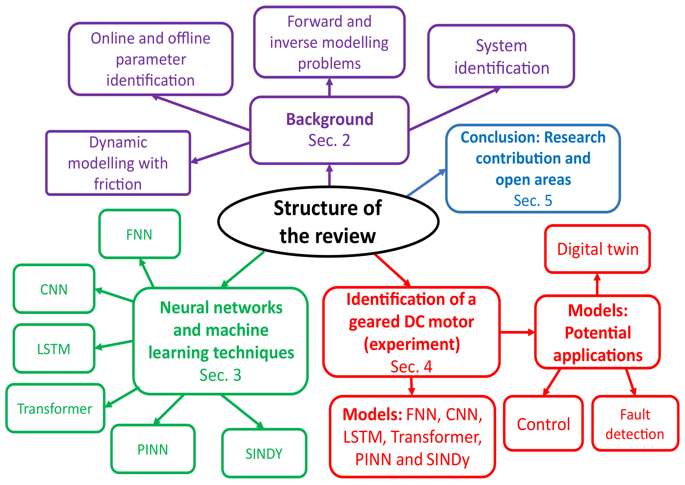
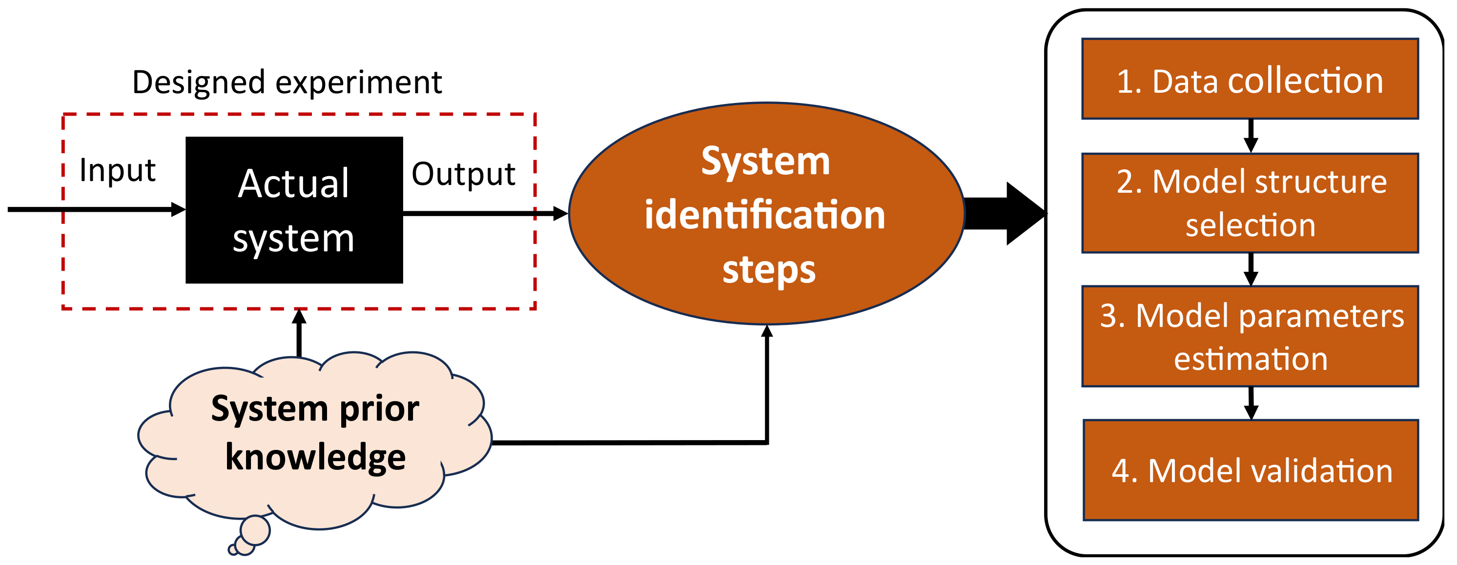
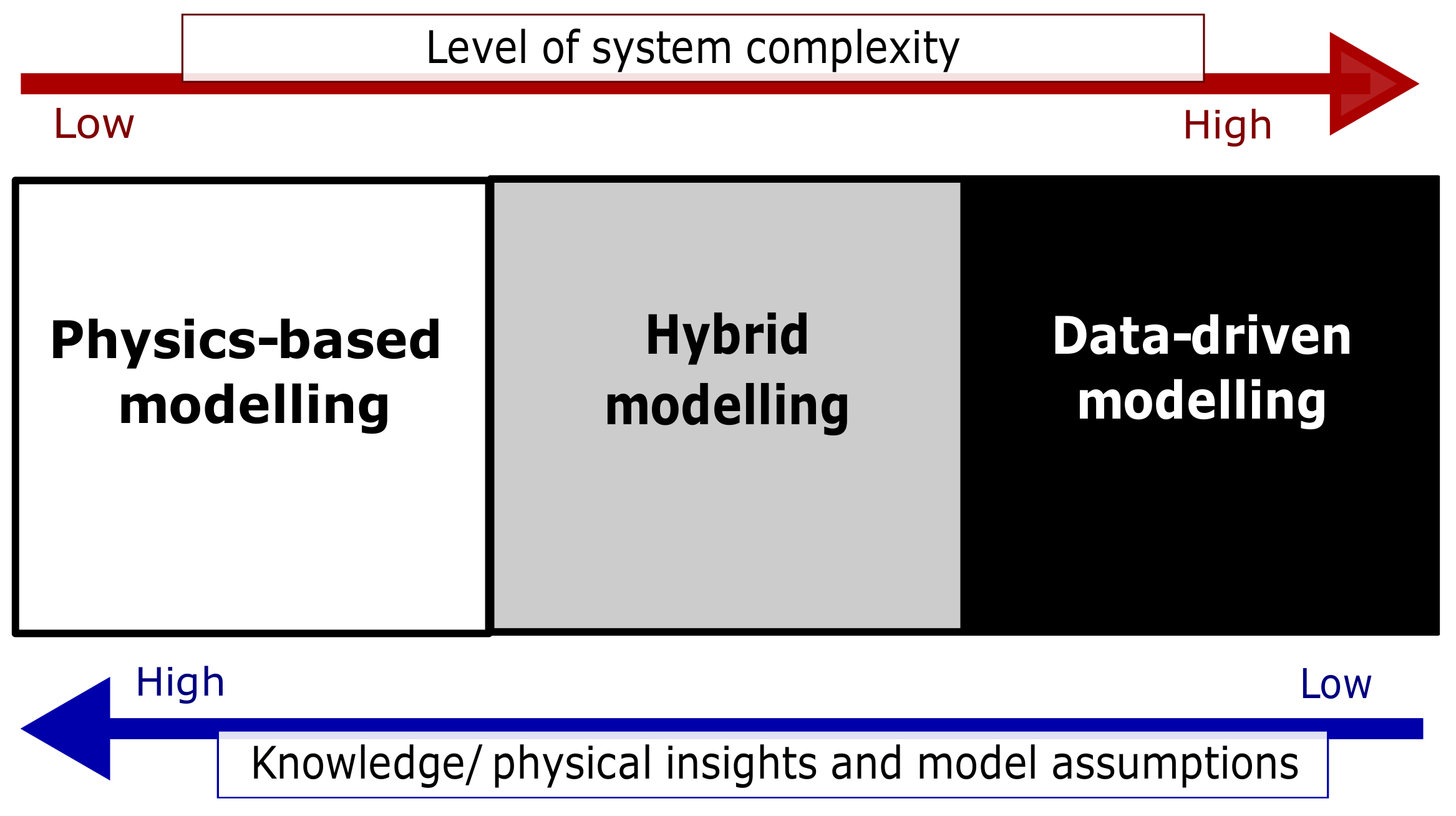
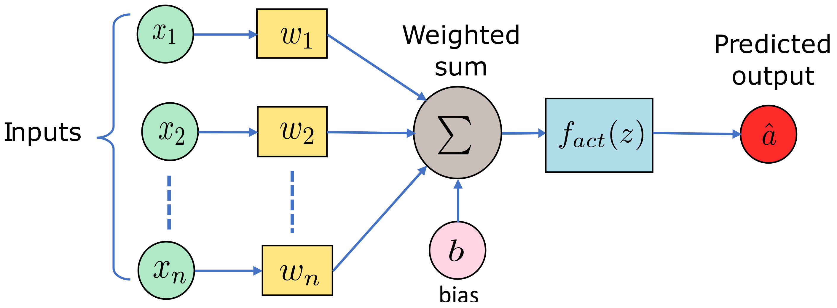
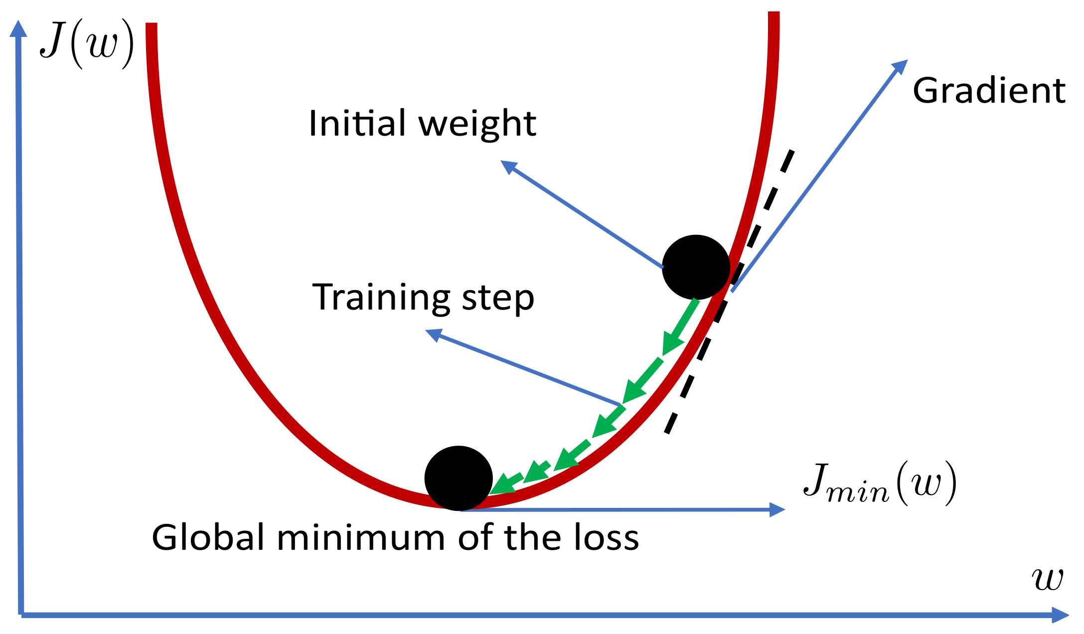
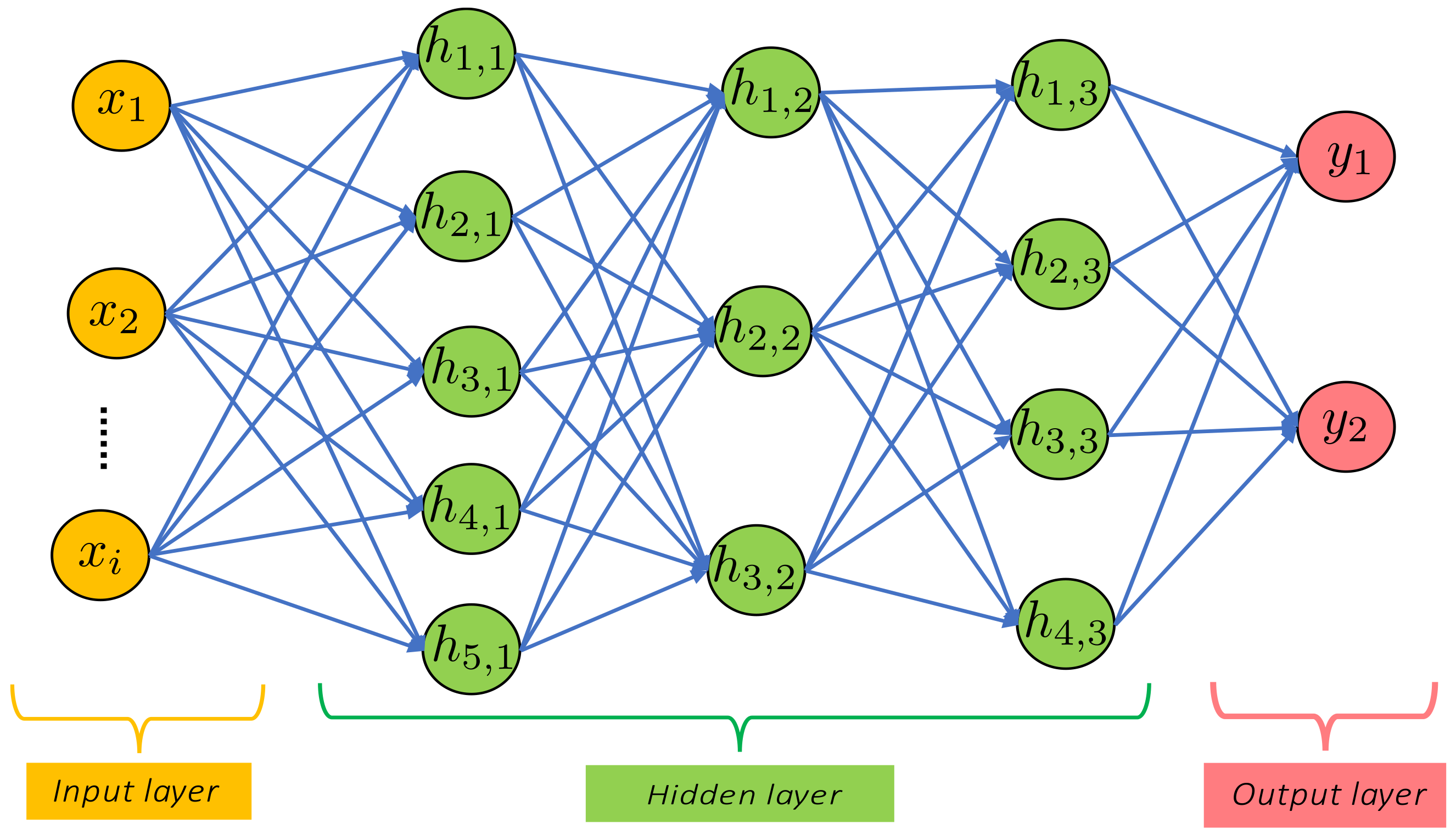
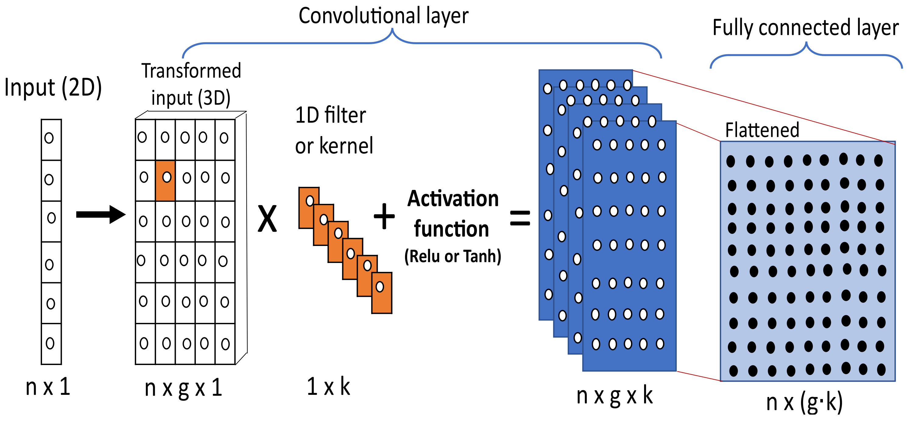

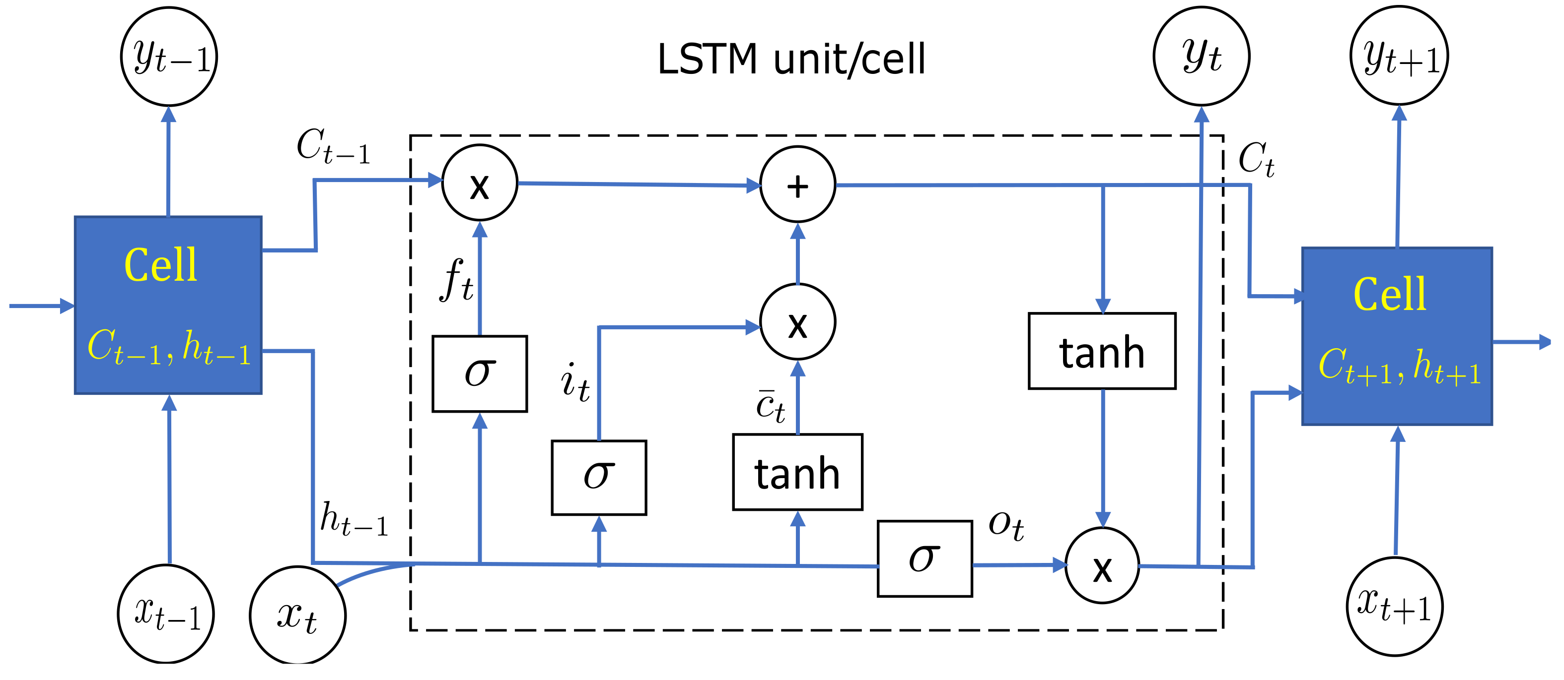
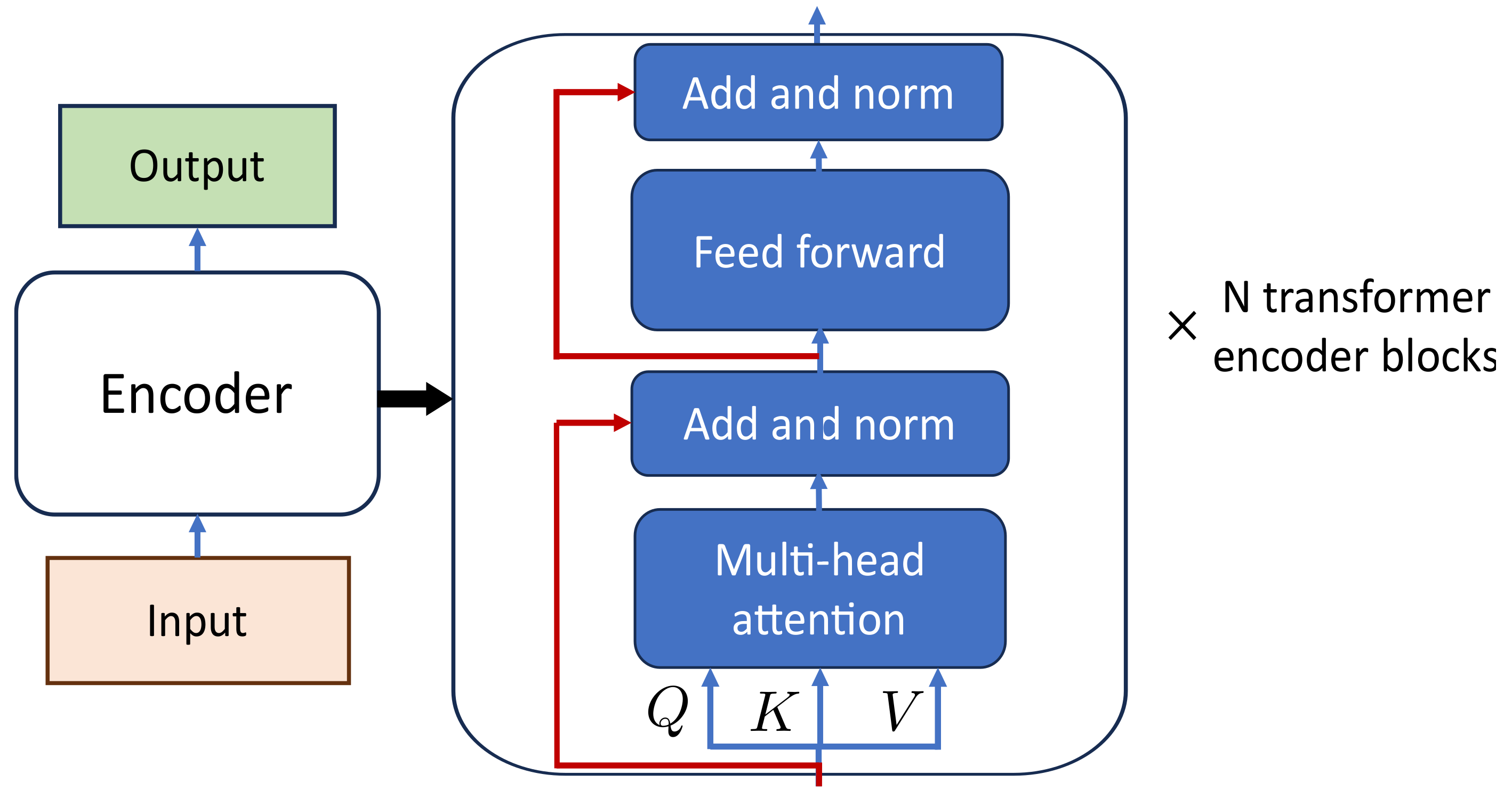
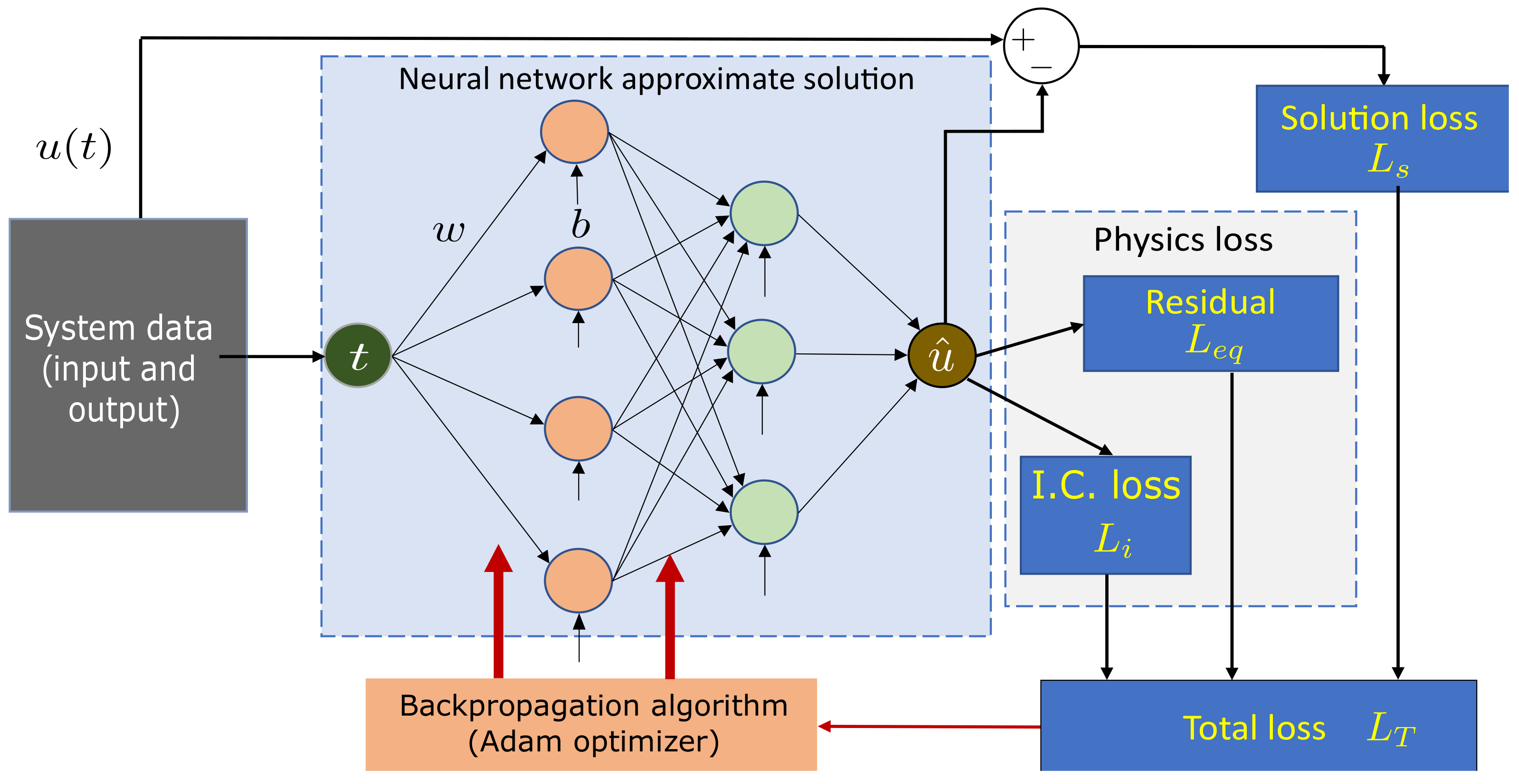

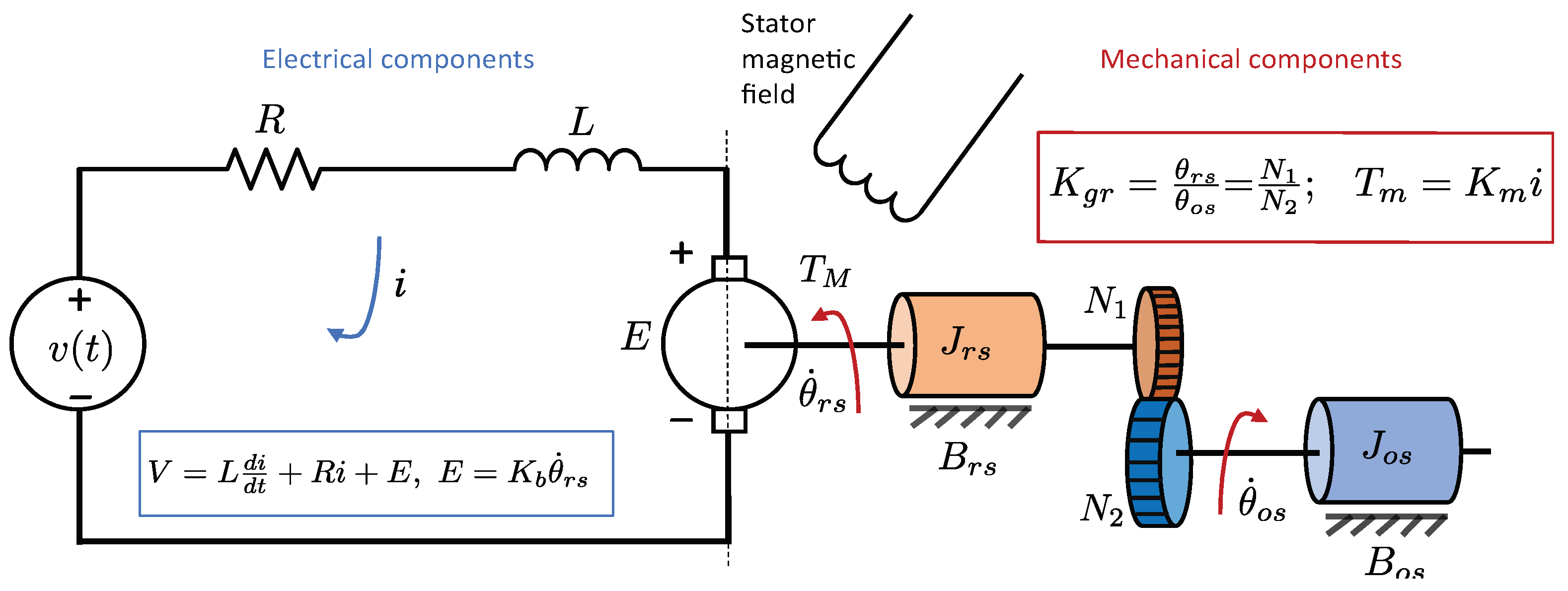
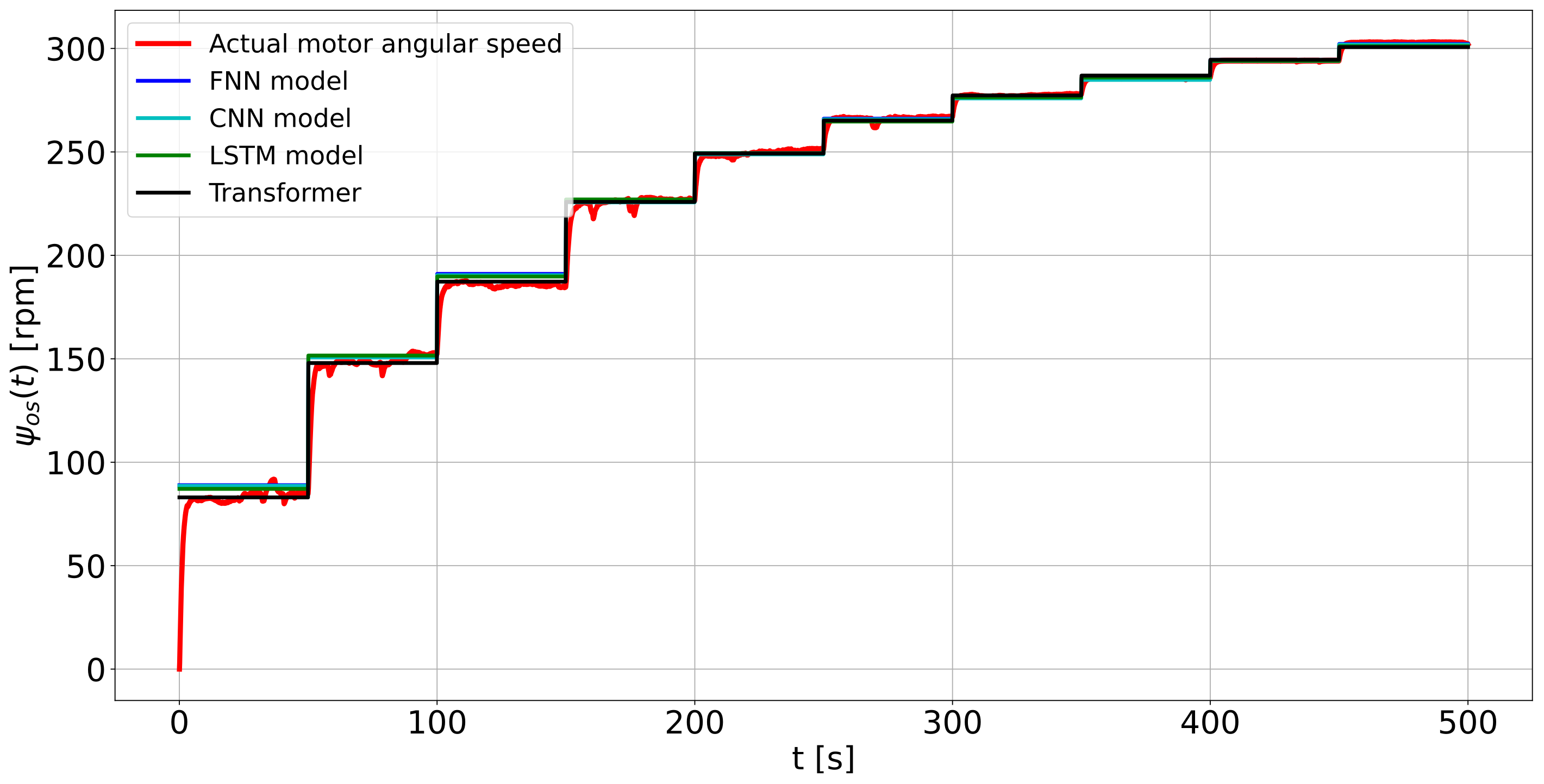


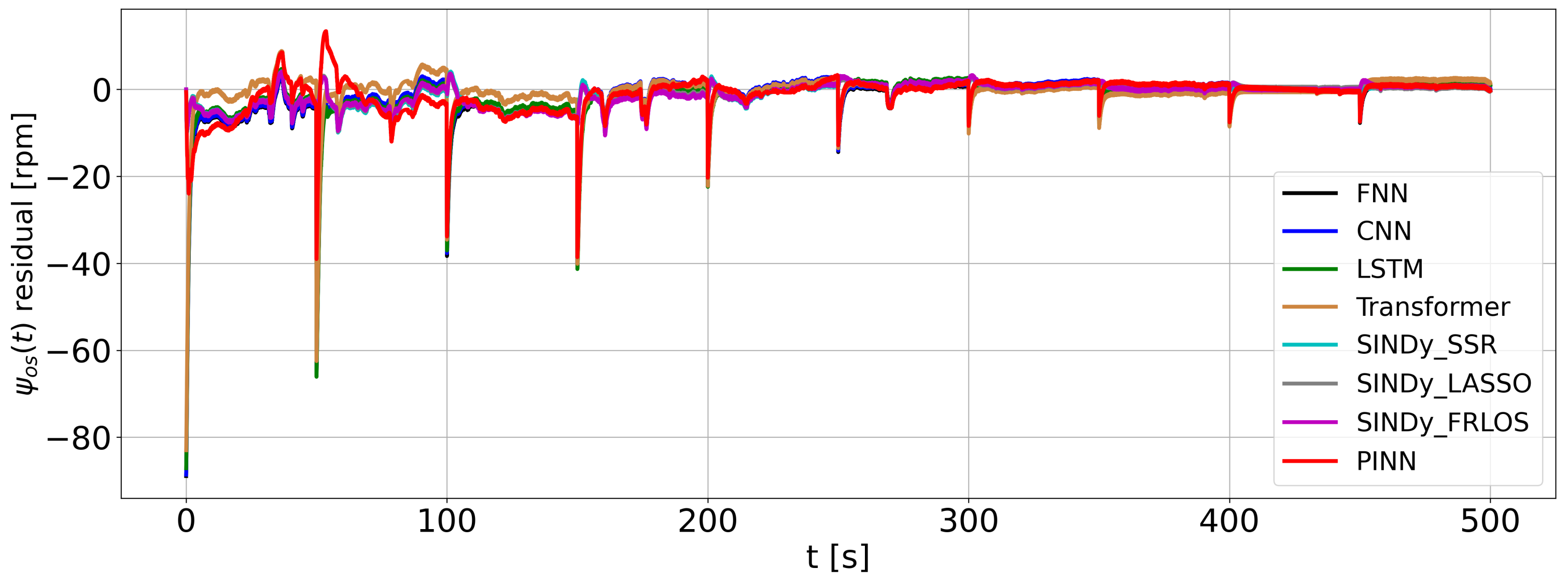

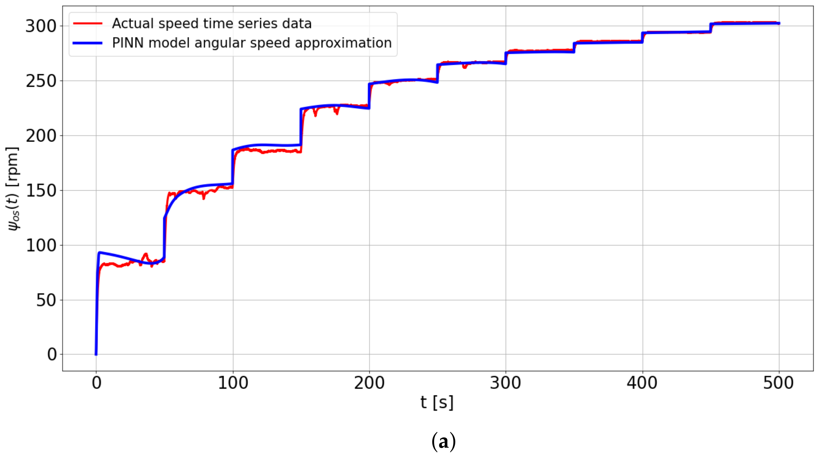
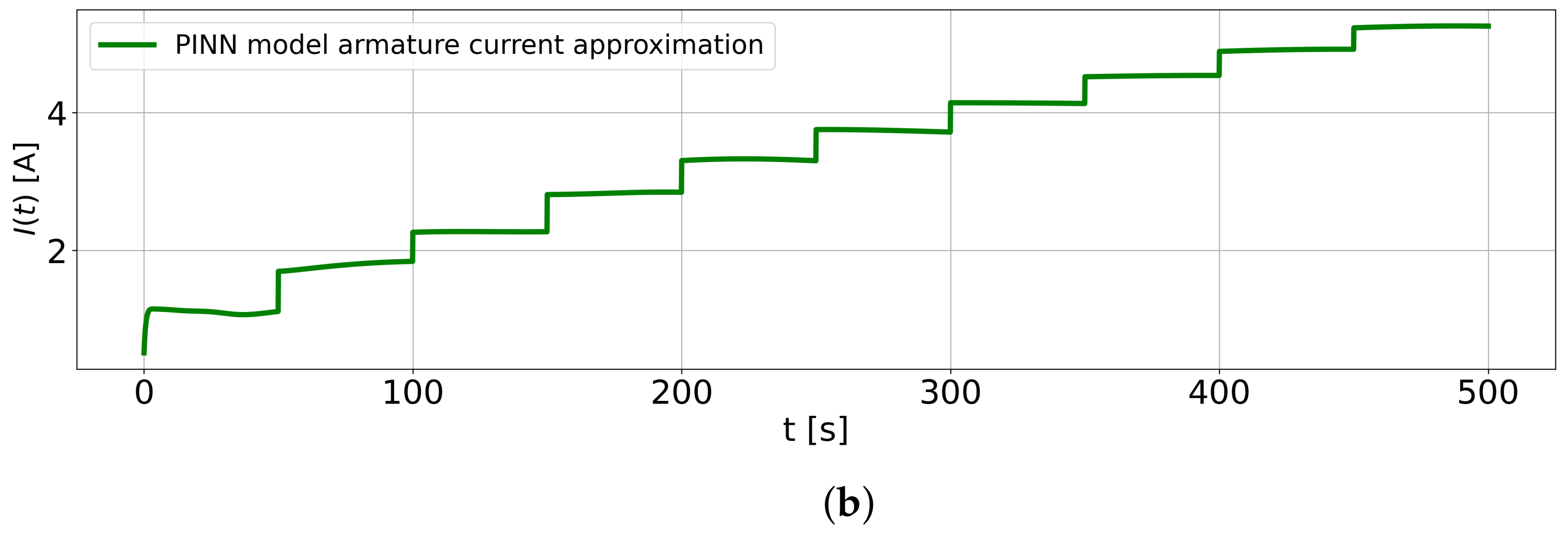