Decentralized QFT Controller Design Based on the Equivalent Subsystems Method

Abstract

Since the 1970s various decentralized control methodologies have been developed to deal with the challenge of controlling complex and/or spatially distributed systems with multiple inputs and multiple outputs (MIMO), e.g., chemical plants, power systems, water systems, etc. In general, the use of distributed information and control structures requires the synthesis of control laws in a constrained (decentralized) information structure. The article presents a novel frequency domain robust decentralized controller design method that is appropriate for uncertain dynamic MIMO systems with equal numbers of input and output variables, which consist of interconnected physical subsystems and are given as a set of square transfer function matrices. The main framework of the proposed method provides the Equivalent Subsystems Method (ESM), whereby the overall closed-loop system under a decentralized controller is stable if, and only if, all the individual closed-loop equivalent subsystems are stable. By generating equivalent subsystems for all transfer matrices, which describe the uncertain MIMO system, the individual uncertain equivalent subsystems are obtained as sets of respective frequency responses. Such representation allows the application of the QFT (quantitative feedback theory) approach to independently design local single-input single-output (SISO) robust controllers which constitute the resulting decentralized controller implemented in real subsystems. The designed controller ensures robust stability of the overall closed-loop system and the required performance as specified by the standard QFT performance specification types in both the equivalent subsystems and the overall closed-loop system. Compared to the existing method and references therein, the proposed method reduces the conservatism of the robust stability conditions and enables the exploitation of the benefits by the SISO QFT approach in the independent design of the robust decentralized controller. The developed design procedure is verified and illustrated in a case study on the robust decentralized level controller design of the quadruple tank process.

1. Introduction

Since it appeared in the 1970s, decentralized control has been an important practice-oriented advanced control approach. Various decentralized control methodologies have been developed to deal with the challenge of controlling complex and/or spatially distributed systems with multiple inputs and multiple outputs (MIMO systems), such as chemical plants, interconnected electrical power systems with strong interactions, water treatment plants, etc.

Typically, complex systems are made up of several mutually interacting subsystems, whereby each subsystem operates relatively independently, with its own sub-objective contributing to the global objective of the overall system. In complex system controls, major problems arise due to interactions among subsystems; if they are strong, multivariable controllers have to be used. Due to practical reasons, restrictions on the controller structure may be reasonable and even inevitable. In the extreme case, when the multivariable controller in the overall system splits into individual local feedback loops, it becomes a decentralized controller. Generally, such constraints on the structure of the controller create a certain performance deterioration compared to centralized controllers; however, these are counterbalanced by significant practical benefits, such as the simplicity of the controller design, as well as hardware, operation, and reliability improvements. Decentralization and decomposition are effective tools to overcome difficulties specific to complex systems, namely, high dimensionality, information structure constraints, and uncertainty [1].

Decentralization has gained a foothold in the development of modern control systems. Distributed control systems are used in the innovative process industries as an extension of traditional controllers. Their major concept is derived from the idea of decentralizing the control unit and establishing a common network between the engineering stations with autonomous controllers distributed throughout the system and a central operator supervisory control [2]. Since the 1980s, as microprocessors became more powerful and cheaper, they could have been embedded in remote devices and components to perform dedicated specific functions, including controlling in a communications network close to the processes they control. In the last few years, the convergence of the cyber and the physical spaces has further transformed traditional embedded systems into cyber–physical systems (CPS), characterized by tight integration and coordination between computation and physical processes through networking. Examples of CPS include a wide range of large-scale engineered systems, such as avionics, healthcare, transportation, and smart grid systems [3]. In general, the use of distributed information and control structures, such as networked systems, embedded systems, or cyber–physical systems, requires the synthesis of control laws in a constrained (decentralized) information structure.

Decentralized control has been the most common control scheme for MIMO systems since the 1970s. Various design approaches and techniques have been developed in both the time and the frequency domains. The first major frequency domain multivariable design techniques were based on a generalization of the classical SISO concepts. In the 1980s, the robust approach to the decentralized control design was commonly used. Key theoretical results in a seminal paper [4] show how the classical SISO statement of the feedback design problem, in the face of uncertainties, can be generalized to MIMO systems. Based on how the interactions between subsystems are handled in the design process, the developed design techniques have been classified as 1. fully coordinated design (simultaneous) design, 2. sequential design, and 3. independent design [5,6,7,8]. According to the first approach, diagonal controllers are designed simultaneously, and the result is theoretically optimal but only offers a few of the decentralized control benefits. The second approach allows the design of local controllers that sequentially apply time decomposition; fast loops are closed first, and the previously designed controllers must be considered when closing subsequent slower loops. However, this approach does not guarantee failure tolerance. In the third approach, each local controller is designed based on the respective decoupled subsystem, such that each local control loop is stable. The resulting diagonal controller guarantees stability and the proper operation of individual parts of the system but at the price of conservative sufficient stability conditions to be met. Usually, off-diagonal interactions cannot be simply neglected; instead, they have to be appropriately considered in the local designs. In industrial practice, decentralized controllers are frequently used with decouplers to minimize interactions or to make the system diagonal dominant, prior to designing local controllers [9,10,11].

In the frequency domain, stability, with respect to model uncertainty (robust stability), is usually assessed by means of stability margins and and sensitivity peaks. However, only a limited number of studies have addressed MIMO controller tuning in terms of gain and phase margins, and these are mostly just for two-input two-output systems and simplified models of decoupled subsystems [12,13]. The Equivalent Subsystems Method (ESM) is a Nyquist-based decentralized controller design method for specified performance [14,15,16], which has been further augmented to integrate the general robust stability condition into its local designs [8,17,18,19]. The method is applicable for uncertain square MIMO systems with arbitrary numbers of subsystems, modeled using unstructured uncertainty. As the method is based on frequency plots, individual subsystems can be of any order, even including unstable zeros and time delays. The design procedure is similar for SISO and MIMO systems, and both continuous and discrete-time controllers.

Likewise, the robust decentralized control method proposed in this article relies on the ESM [17], according to which the overall closed-loop system under a decentralized controller is stable if, and only if, all individual closed-loop equivalent subsystems are stable. By generating equivalent subsystems for all transfer matrices from the set describing the uncertain MIMO system, individual uncertain equivalent subsystems are obtained as sets of respective frequency responses. Such a representation allows the application of the QFT (quantitative feedback theory) approach, described in [20], to independently design local single-input single-output (SISO) robust controllers, which constitute the resulting decentralized controller implemented in real subsystems. Due to the use of the QFT performance specification types in the design of local controllers for equivalent subsystems, the resulting robust decentralized controller ensures robust stability and the required performance for the overall closed-loop system. The main benefits brought about by the integration of the ESM and QFT methods are two-fold: reduced design conservatism because there is no need to consider an unnecessarily broader uncertainty domain due to the necessity of using unstructured uncertainty modeli when integrating the general robust stability in local designs. Secondly, the possibility to specify nearly arbitrary performance requirements for the overall system and ensure their fulfillment by translating them into frequency domain specifications for equivalent subsystems. Not least, the proposed design procedure is universal and simple to use compared to the two MIMO QFT design approaches, presented in [20], which are basically sequential designs, while other existing QFT-based decentralized controllers are case-specific, e.g., [21,22].

The article is organized as follows: Section 2 provides a concise theoretical background on the topic and formulates the problem to be solved. In Section 3, the principles of the ESM and the standard QFT compensator design are presented; these two methods are synergically integrated into the proposed robust decentralized controller design method presented in Section 4. The developed design procedure is demonstrated in detail and verified by a case study on the robust decentralized controller design for the quadruple tank process [23] in Section 5. Based on the achieved results, the benefits and limitations of the developed method are summarized and generalized in Section 6.

2. Preliminaries and Problem Formulation

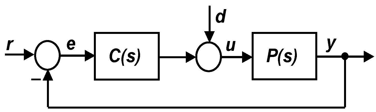
Consider the standard closed-loop in Figure 1, where P(s) is a $m\times m$ transfer function matrix modeling the controlled plant with m inputs and m outputs, $\mathrm{m}\ge 1,$ and C(s) is a $m\times m$ transfer function matrix of a controller; r, e, u, y, and d denote the reference, control error, control action, output, and input disturbance variables, respectively.

The necessary and sufficient stability conditions for the MIMO closed-loop are expressed in the generalized Nyquist stability theorem.

Theorem 1

(Generalized Nyquist stability theorem [5]). Suppose that P(s) and C(s) are minimal realizations of a MIMO system and a controller, respectively. Then, the closed-loop in Figure 1 is internally stable if and only if $\forall s\in \mathcal{D}:$

$$1. \det \left[\mathrm{I}+\mathrm{Q}\left(\mathrm{s}\right)\right]\ne 0$$

(1)

$$2. \mathrm{N}\left\{0,\det \left[\mathrm{I}+\mathrm{Q}\left(\mathrm{s}\right)\right]\right\}={\displaystyle \sum }_{\mathrm{i}=1}^{\mathrm{m}}\mathrm{N}\left\{0,\left[1+{\mathrm{q}}_{\mathrm{i}}\left(\mathrm{s}\right)\right]\right\}={\mathrm{n}}_{\mathrm{q}},$$

(2)

where $Q\left(s\right)=P\left(s\right)C\left(s\right)$ is the open-loop transfer function with no internal right half-plane pole-zero cancellations between $P\left(s\right)$ and $C\left(s\right); N\left\{0,\mathit{det}\left[I+Q\left(s\right)\right]\right\}$ is the number of anticlockwise encirclements of (0,0j) by $\mathit{det}\left[I+Q\left(s\right)\right]; n_q$ is the number of unstable poles of $Q\left(s\right);$ $\mathcal{D}$ is the Nyquist contour; I is the identity matrix; $q_i\left(s\right), i=1,\dots , m$ are characteristic functions of $Q\left(s\right)$ defined as:

$$\det \left[{\mathrm{q}}_{\mathrm{i}}\left(s\right)\mathrm{I}-\mathrm{Q}\left(\mathrm{s}\right)\right]=0, \mathrm{i}=1,\dots , \mathrm{m}.$$

(3)

Remark 1.

The Nyquist contour $\mathcal{D}$ is a large contour in the complex plain consisting of the imaginary axis $s=j\omega , \omega ϵ〈-\alpha , \alpha 〉$, where $\alpha$ is the radius of a semicircle in the right half-plane, large enough to encircle unstable poles of $Q\left(s\right)$; if there are any poles in the imaginary axis, $\mathcal{D}$ is intended to the left-half plane to include them.

Remark 2.

Characteristic loci (CL) $q_i\left(j\omega \right), i=1,\dots , m$ are traced out in the complex plane by characteristic functions of Q(s) as s traverses the Nyquist contour $\mathcal{D}$.

Let the mathematical description of an uncertain MIMO plant with an equal number of inputs and outputs be given as a set of square transfer matrices; such a specification is used if the MIMO system has been identified in several (N) working points.

The set $\mathsf{\Pi }$ of transfer matrices is given as:

$$\mathsf{\Pi }:\left\{{\mathrm{P}}^{\mathrm{k}}\left(\mathrm{s}\right)\right\}, \mathrm{k}=1,\dots ,\mathrm{N},$$

(4)

where

$${\mathrm{P}}^{\mathrm{k}}\left(\mathrm{s}\right)=\left\{{\mathrm{P}}_{\mathrm{ij}}^{\mathrm{k}}\left(\mathrm{s}\right)\right\}, \mathrm{i},\mathrm{j}=1,\dots , \mathrm{m}, \mathrm{m}\ge 1,$$

(5)

and individual entries in the transfer matrix (5) are in the general form:

$${\mathrm{P}}_{\mathrm{ij}}^{\mathrm{k}}\left(\mathrm{s}\right)=\frac{{\mathrm{B}}_{\mathrm{ij}}^{\mathrm{k}}\left(\mathrm{s}\right)}{{\mathrm{A}}_{\mathrm{ij}}^{\mathrm{k}}\left(\mathrm{s}\right)}=\frac{{\sum }_{\mathrm{q}=0}^{\mathrm{r}}{\mathrm{b}}_{\mathrm{ijq}}^{\mathrm{k}}{\mathrm{s}}^{\mathrm{q}}}{{\sum }_{\mathrm{p}=0}^{\mathrm{n}}{\mathrm{a}}_{\mathrm{ijp}}^{\mathrm{k}}{\mathrm{s}}^{\mathrm{p}}}, \mathrm{q}=1,\dots ,\mathrm{r};\mathrm{p}=1,\dots ,\mathrm{n}; \mathrm{r}<\mathrm{n}.$$

(6)

The uncertain system (4) can be modeled using the nominal model and a suitable uncertainty model that properly quantifies the difference between the real and the nominal system dynamics. The nominal model:

$${\mathrm{P}}^0\left(\mathrm{s}\right)=\left\{{\mathrm{P}}_{\mathrm{ij}}^0\left(\mathrm{s}\right)\right\}, \mathrm{i},\mathrm{j}=1,\dots ,\mathrm{m},$$

(7)

is usually obtained as a mean value parameter model [5,6,17] or can simply be selected as any from the set of transfer matrices (4), [20].

The uncertainty can be described as parametric (structured) or nonparametric (unstructured) [5]. When nonparametric uncertainty is considered, the set $\mathsf{\Pi }$ is generated using any of the six types of unstructured uncertainty models [5,17] and the upper bound on its spectral norm. In the case of parametric uncertainty, knowledge of the structure of all elements of $\mathsf{\Pi }$ is assumed, while their parameters may vary within a given compact set.

Using parametric uncertainty, the uncertain SISO system is described by (4), where individual entries (6) have a uniform structure ($\mathrm{i}=1, \mathrm{j}=1, \mathrm{m}=1$ and the superscript k is omitted for readability):

$$\mathrm{P}\left(\mathrm{s}\right)=\frac{\mathrm{B}\left(\mathrm{s}\right)}{\mathrm{A}\left(\mathrm{s}\right)}=\frac{{\mathrm{a}}_0+{ \mathrm{a}}_1\mathrm{s}+{ \mathrm{a}}_2{\mathrm{s}}^2+\dots +{\mathrm{a}}_{\mathrm{n}}{\mathrm{s}}^{\mathrm{n}}}{{\mathrm{b}}_0+{ \mathrm{b}}_1\mathrm{s}+{ \mathrm{b}}_2{\mathrm{s}}^2+\dots +{\mathrm{b}}_{\mathrm{m}}{\mathrm{s}}^{\mathrm{m}}}, {\mathrm{a}}_{\mathrm{n}}\ne 0,{ \mathrm{b}}_{\mathrm{m}}\ne 0, \mathrm{m}\le \mathrm{n},$$

(8)

with varying coefficients of numerator and denominator polynomials.

The interval polynomials of the numerator and denominator are defined by means of the lower and upper limits of their uncertain coefficients as follows:

$$\begin{array}{c}\mathrm{D}\left(\mathrm{s}\right)=\left\{\mathrm{A}\left(\mathrm{s}\right):{\mathrm{a}}_0+\dots +{\mathrm{a}}_{\mathrm{n}}{\mathrm{s}}^{\mathrm{n}},{\mathrm{a}}_{\mathrm{k}}\in \langle \underset{¯}{{\mathrm{a}}_{\mathrm{k}}},\overline{{\mathrm{a}}_{\mathrm{k}}}\rangle ,\mathrm{k}=0,1,2,\dots ,\mathrm{n}\right\}\\ \mathrm{N}\left(\mathrm{s}\right)=\left\{\mathrm{B}\left(\mathrm{s}\right):{\mathrm{b}}_0+\dots +{\mathrm{b}}_{\mathrm{m}}{\mathrm{s}}^{\mathrm{m}},{\mathrm{b}}_{\mathrm{k}}\in \langle \underset{¯}{{\mathrm{b}}_{\mathrm{k}}},\overline{{\mathrm{b}}_{\mathrm{k}}}\rangle ,\mathrm{k}=0,1,2,\dots ,\mathrm{m}\right\}.\end{array}$$

(9)

Then, the corresponding interval system reads as:

$$\mathrm{P}\left(\mathrm{s}\right):=\left\{\mathrm{P}\left(\mathrm{s}\right)=\frac{\mathrm{n}\left(\mathrm{s}\right)}{\mathrm{d}\left(\mathrm{s}\right)}: \mathrm{n}\left(\mathrm{s}\right)ϵ\mathrm{N}\left(\mathrm{s}\right), \mathrm{d}\left(\mathrm{s}\right)ϵ\mathrm{D}\left(\mathrm{s}\right)\right\}$$

(10)

A controller that guarantees closed-loop stability over the whole uncertainty region, defined by the set of uncertain plant models (4) and modeled using a selected type of uncertainty (parametric uncertainty in our case), is called a robust controller. Being designed for the nominal model selected from the set (4), the robust controller has to first guarantee nominal stability. Thus, nominal stability is a prerequisite for robust stability.

The main results of the parametric approach in robust control evolve from Kharitonov’s theorem, which provides a necessary and sufficient condition of robust stability for an interval family of polynomials. An overview of the robust analysis results, generalization of Kharitonov’s theorem, the Edge theorem, and the related results can be found, e.g., in [24].

The frequency-domain QFT controller design methodology presented in [20], and references therein, allows for the synthesis of a compensator that guarantees closed-loop robust stability in the interval system (10), while also respecting the bounds imposed by performance requirements. In the subsequent study, we will build on this approach.

Consider the uncertain MIMO system (4), which is an interconnection of $\mathrm{m}$ subsystems that has $\mathrm{m}$ inputs and $\mathrm{m}$ outputs; this type of uncertain MIMO system can be modeled as a set of square transfer function matrices (5):

$${\mathrm{P}}^{\mathrm{k}}\left(\mathrm{s}\right)=\left[\begin{array}{cccc}{\mathrm{P}}_{11}^{\mathrm{k}}\left(\mathrm{s}\right)& {\mathrm{P}}_{12}^{\mathrm{k}}\left(\mathrm{s}\right)& \cdots & {\mathrm{P}}_{1\mathrm{m}}^{\mathrm{k}}\left(\mathrm{s}\right)\\ {\mathrm{P}}_{21}^{\mathrm{k}}\left(\mathrm{s}\right)& {\mathrm{P}}_{22}^{\mathrm{k}}\left(\mathrm{s}\right)& \cdots & {\mathrm{P}}_{2\mathrm{m}}^{\mathrm{k}}\left(\mathrm{s}\right)\\ ⋮& ⋮& ⋮& ⋮\\ {\mathrm{P}}_{\mathrm{m}1}^{\mathrm{k}}\left(\mathrm{s}\right)& \cdots & \cdots & {\mathrm{P}}_{\mathrm{mm}}^{\mathrm{k}}\left(\mathrm{s}\right)\end{array}\right], \mathrm{k}=1,\dots , \mathrm{N}; \mathrm{m}\ge 1.$$

(11)

To design a robust decentralized controller, the transfer matrices (11) have to be recast into a single transfer matrix, for which entries are in the form of interval systems (8)–(10).

To design a decentralized controller, all transfer matrices (11) will be split according to regular splitting [25], as follows (the superscript $\mathrm{k}$ is omitted for simplicity):

$$\mathrm{P}\left(\mathrm{s}\right)={\mathrm{P}}_{\mathrm{d}}\left(\mathrm{s}\right)+{\mathrm{P}}_{\mathrm{n}}\left(\mathrm{s}\right),$$

(12)

where the nonsingular diagonal matrix

$${\mathrm{P}}_{\mathrm{d}}\left(\mathrm{s}\right)=\left[\begin{array}{cccc}{\mathrm{P}}_{11}\left(\mathrm{s}\right)& 0& \cdots & 0\\ 0& {\mathrm{P}}_{22}\left(\mathrm{s}\right)& \cdots & 0\\ ⋮& ⋮& ⋮& ⋮\\ 0& \cdots & \cdots & {\mathrm{P}}_{\mathrm{mm}}\left(\mathrm{s}\right)\end{array}\right]$$

(13)

describes the dynamics of the decoupled subsystems, and the off-diagonal entries collected in ${\mathrm{P}}_{\mathrm{n}}\left(\mathrm{s}\right)=\mathrm{P}\left(\mathrm{s}\right)-{\mathrm{P}}_{\mathrm{d}}\left(\mathrm{s}\right)$ correspond to interactions.

2.1. Problem Formulation

Consider an uncertain MIMO system with $\mathrm{m}$ inputs and $\mathrm{m}$ outputs consisting of m subsystems, $\mathrm{m}\ge 1,$ given as a set of $\mathrm{N}$ transfer function matrices (4), whereby each transfer function matrix can be split into the diagonal and off-diagonal transfer matrices, ${\mathrm{P}}_{\mathrm{d}}^{\mathrm{k}}\left(\mathrm{s}\right)$ and ${\mathrm{P}}_{\mathrm{n}}^{\mathrm{k}}\left(\mathrm{s}\right)$, respectively:

$${\mathrm{P}}^{\mathrm{k}}\left(\mathrm{s}\right)={ \mathrm{P}}_{\mathrm{d}}^{\mathrm{k}}\left(\mathrm{s}\right)+{ \mathrm{P}}_{\mathrm{n}}^{\mathrm{k}}\left(\mathrm{s}\right), \mathrm{k}=1,\dots \mathrm{N},$$

(14)

where ${\mathrm{P}}_{\mathrm{d}}^{\mathrm{k}}\left(\mathrm{s}\right)$ and ${\mathrm{P}}_{\mathrm{m}}^{\mathrm{k}}\left(\mathrm{s}\right)$ are the transfer matrices in decoupled subsystems and the interactions among them, respectively.

A decentralized (diagonal) controller (15)

$$\mathrm{C}\left(\mathrm{s}\right)=\mathrm{diag}\left\{{\mathrm{C}}_{\mathrm{i}}\left(\mathrm{s}\right)\right\}, \mathrm{i}=1,\dots ,\mathrm{m}; \det \mathrm{C}\left(\mathrm{s}\right)\ne 0, \forall \mathrm{s}$$

(15)

has to be designed to guarantee closed-loop stability and provide the required performance over the whole operating range of the uncertain system (4).

The design problem will be solved in the frequency domain as an independent design, based on the Equivalent Subsystems Method [17], to allow parametric uncertainty to be considered in the design of local controllers as well as properly formulated performance requirements.

3. Methods Applied in the Solution

To solve the robust decentralized controller design problem formulated in Section 2.1, a design procedure was developed based on two frequency-domain design methodologies:

• the Equivalent Subsystem Method (ESM), which provides a framework for the independent design of local controllers constituting the decentralized controller to guarantee closed-loop stability of the overall system;
• the quantitative feedback theory (QFT), to design a minimum structure of local compensators guaranteeing robust stability of uncertain SISO systems with parametric uncertainty as well as fulfillment of properly specified performance requirements.

Both methods are graphical and based on nonparametric models of the controlled system and related frequency dependencies. Thus, the design procedure is graphical, insightful, and interactive, and even intermediate results have an immediate visual interpretation.

3.1. The Equivalent Subsystems Method

The Equivalent Subsystems Method (ESM) is a Nyquist-based decentralized controller design method for stability and specified performance. It relies on the factorization of the closed-loop characteristic polynomial of the feedback system in Figure 1:

$$\det \left[\mathrm{I}+\mathrm{P}\left(\mathrm{s}\right)\mathrm{C}\left(\mathrm{s}\right)\right]=\det \left[{\mathrm{C}}^{-1}\left(\mathrm{s}\right)+{\mathrm{P}}_{\mathrm{d}}\left(\mathrm{s}\right)+{\mathrm{P}}_{\mathrm{n}}\left(\mathrm{s}\right)\right]\mathrm{detC}\left(\mathrm{s}\right)$$

(16)

where $\mathrm{C}\left(\mathrm{s}\right)$ is a decentralized (diagonal) controller (15).

Characteristic functions ${\mathrm{g}}_{\mathrm{i}}\left(\mathrm{s}\right), \mathrm{i}=1,2,\dots ,\mathrm{m}$ of ${\mathrm{P}}_{\mathrm{n}}\left(\mathrm{s}\right)$ are defined as follows:

$$\det \left[{\mathrm{g}}_{\mathrm{i}}\left(\mathrm{s}\right)\mathrm{I}-{\mathrm{P}}_{\mathrm{n}}\left(\mathrm{s}\right)\right]=0, \mathrm{i}=1,\dots ,\mathrm{m}.$$

(17)

In terms of stability, ${\mathrm{P}}_{\mathrm{n}}\left(\mathrm{s}\right)$ can be replaced by its characteristic function matrix according to the Cayley–Hamilton Theorem:

$${\mathrm{P}}_{\mathrm{n}}\left(\mathrm{s}\right)={\mathrm{g}}_{\mathrm{k}}\left(\mathrm{s}\right)\mathrm{I}, \mathrm{k}\in \left\{1,\dots ,\mathrm{m}\right\},$$

(18)

where ${\mathrm{g}}_{\mathrm{k}}\left(\mathrm{s}\right), \mathrm{k}\in \left\{1,\dots ,\mathrm{m}\right\}$ is one (arbitrary) selected characteristic function.

As a result, (16) modifies to:

$$\mathrm{N}\left\{0,\det \left[\mathrm{I}+\mathrm{P}\left(\mathrm{s}\right)\mathrm{C}\left(\mathrm{s}\right)\right]\right\}=\mathrm{N}\left\{0,\det \left[{\mathrm{C}}^{-1}\left(\mathrm{s}\right)+{\mathrm{P}}_{\mathrm{d}}\left(\mathrm{s}\right)+{\mathrm{g}}_{\mathrm{k}}\left(\mathrm{s}\right)\mathrm{I}\right]\mathrm{detC}\left(\mathrm{s}\right)\right\}.$$

(19)

Using the following notation in the bracketed term on the right-hand side:

$${\mathrm{P}}_{\mathrm{k}}^{\mathrm{eq}}\left(\mathrm{s}\right):={\mathrm{P}}_{\mathrm{d}}\left(\mathrm{s}\right)+{\mathrm{g}}_{\mathrm{k}}\left(\mathrm{s}\right)\mathrm{I}=\mathrm{diag}\left\{{\mathrm{P}}_{\mathrm{ik}}^{\mathrm{eq}}\left(\mathrm{s}\right)\right\}, \mathrm{i}=1,2,\dots , \mathrm{m}; \mathrm{k}\in \left\{1,\dots ,\mathrm{m}\right\},$$

(20)

the diagonal matrix of equivalent subsystems is defined by (20).

Since the analytical calculation of characteristic functions is not straightforward and sometimes even unfeasible, they are computed frequency-by-frequency, which results in individual equivalent subsystems being generated according to:

$${\mathrm{P}}_{\mathrm{ik}}^{\mathrm{eq}}\left(\mathrm{j}\mathsf{\omega }\right)={\mathrm{P}}_{\mathrm{ii}}\left(\mathrm{j}\mathsf{\omega }\right)+{\mathrm{g}}_{\mathrm{k}}\left(\mathrm{j}\mathsf{\omega }\right), \mathrm{i}=1,2,\dots ,\mathrm{m}, \mathrm{k}\in \left\{1,2,\dots ,\mathrm{m}\right\}, \forall \mathrm{j}\mathsf{\omega }\in \mathcal{D}$$

(21)

which are frequency responses of individual decoupled subsystems, shaped by a selected characteristic locus of the matrix of interactions.

Substituting (20) into (19) after a small manipulation yields the key result:

$$\mathrm{N}\left\{0,\det \left[\mathrm{I}+\mathrm{P}\left(\mathrm{s}\right)\mathrm{C}\left(\mathrm{s}\right)\right]\right\}=\mathrm{N}\left\{0,\det \left[\mathrm{I}+{\mathrm{P}}_{\mathrm{k}}^{\mathrm{eq}}\left(\mathrm{s}\right)\mathrm{C}\left(\mathrm{s}\right)\right]\right\}.$$

(22)

Considering (21), further manipulation of the r.h.s. of (22) results in:

$$\mathrm{N}\left\{0,\det \left[\mathrm{I}+{\mathrm{P}}_{\mathrm{k}}^{\mathrm{eq}}\left(\mathrm{s}\right)\mathrm{C}\left(\mathrm{s}\right)\right]\right\}={\displaystyle \sum }_{\mathrm{i}=1}^{\mathrm{m}}\mathrm{N}\left\{-1,\left[{\mathrm{P}}_{\mathrm{ii}}\left(\mathrm{s}\right)+{\mathrm{g}}_{\mathrm{k}}\left(\mathrm{s}\right)\right]{\mathrm{C}}_{\mathrm{i}}\left(\mathrm{s}\right)\right\}={\mathrm{n}}_{\mathrm{q}}$$

(23)

From (22) and (23) results that the necessary and sufficient conditions for the closed-loop stability of the overall system under a decentralized controller are guaranteed if and only if each closed-loop equivalent subsystem under its related local controller is stable. The above development is summarized in Theorem 2, which reformulates the conditions of the generalized Nyquist stability theorem (Theorem 1) for a MIMO system under a decentralized controller.

Theorem 2.

(Stability of a MIMO system under a decentralized controller [17]). The closed-loop in Figure 1 comprising a MIMO system (11) and a decentralized controller (15) is stable if, and only if, there exists $g_k\left(j\omega \right),$ such that $\forall s=j\omega \in \mathcal{D}$

$$\begin{array}{c}1. \det \left[{\mathrm{g}}_{\mathrm{k}}\left(\mathrm{j}\mathsf{\omega }\right)\mathrm{I}-{\mathrm{P}}_{\mathrm{n}}\left(\mathrm{j}\mathsf{\omega }\right)\right]=0, \mathrm{k}\in \left\{1,2,\dots ,\mathrm{m}\right\}\\ 2. \sum _{i=1}^m\mathrm{N}\left\{-1,\left[{\mathrm{P}}_{\mathrm{ii}}\left(\mathrm{j}\mathsf{\omega }\right)+{\mathrm{g}}_{\mathrm{k}}\left(\mathrm{j}\mathsf{\omega }\right)\right]{\mathrm{C}}_{\mathrm{i}}\left(\mathrm{j}\mathsf{\omega }\right)\right\}={\mathrm{n}}_{\mathrm{q}}.\end{array}$$

(24)

Proof of Theorem 2 results from the above development based on Equations (16)–(23) and can also be found in [17].

Theorem 2 implies that a decentralized controller guaranteeing stability of the overall closed-loop system is composed of local controllers independently designed for individual equivalent subsystems using any SISO design. The ESM-based decentralized controller design is applicable for square MIMO systems of any dimension with stable interactions. By integrating robust stability conditions into local controller designs, it can be extended to design robust controllers.

Since equivalent subsystems are generated in the form of frequency characteristics, the following frequency domain design methods are recommended:

• The Neymark D-partition method [15,16] is suitable if performance requirements for the overall system are specified in terms of its degree of stability; the same degrees of stability must be achieved in equivalent subsystems. Using this SISO design, robust stability conditions cannot be directly incorporated in the design of local controllers, they can only be checked additionally, which makes the robust controller design iterative.
• Standard Bode diagram design [8,18] or the Nyquist diagram design [14]. Performance requirements for the overall system, specified in terms of maximum overshoot and settling time, have to be translated into respective frequency performance measures (stability margins) to be achieved in individual equivalent subsystems. Robust stability conditions for systems with unstructured uncertainty can be easily incorporated into local designs [8,17].
• Nichols diagram-based SISO design known as a well-elaborated QFT design technique is the next option, which allows dealing with uncertain systems with parametric uncertainty.

3.2. QFT Design

The quantitative feedback theory (QFT) is a frequency domain engineering method that is used to design robust controllers, developed by Isaac Horowitz [8], the founder of an important scientific school. This robust feedback compensator synthesis methodology is based on classical feedback control theory and simultaneously allows 1. the reduction of the impact of model uncertainty, while 2. satisfying properly specified performance requirements for each realization of a given set of uncertain systems.

QFT solves the above problems by designing a single (robust) compensator capable of simultaneously achieving multiple desired performance specifications (including stability, rejection of input and output disturbances, limitation of control variable, reference variable tracking, damping of oscillation, etc.) for every plant within the existing model uncertainty. It highlights the trade-off (quantification) among the simplicity of the controller structure, minimization of the ‘cost of feedback’ (bandwidth), model uncertainty (parametric and nonparametric), and the achievement of the desired performance specifications at every frequency of interest [26]. As a frequency method, QFT uses frequency tools that are illustrative and understandable by practitioners at each step of the design process.

The standard SISO QFT controller design procedure has the following steps [20]:

• Plant modeling, which includes the specification of the interval model and appropriate frequency range.
• Definition of a discrete number of plants, choice of the nominal model.
  By gridding each uncertain parameter of the interval model between its minimum and maximum values, another set of uncertain plant realizations is generated from all combinations of uncertain parameter values. The task is simplified if the uncertain parameters are interrelated with each other. Any model from the generated plant realizations can be selected as the nominal one; the final QFT controller will be the same no matter what nominal plant is chosen [20].
• Calculation of QFT templates.
  QFT templates are projections of the transfer function $\mathrm{P}\left(\mathrm{j}\mathsf{\omega }\right)$ onto the Nichols diagram, considering each parameter within the uncertainty and at each frequency ω of interest.
• Stability specifications.
  Instead of using classical gain and phase stability margins, ${\mathrm{M}}_{\mathrm{c}}$ circles are used as a more general stability measure representing the loci of constant closed-loop magnitudes ${\mathrm{W}}_{\mathrm{s}}$ in the Nichols diagram.
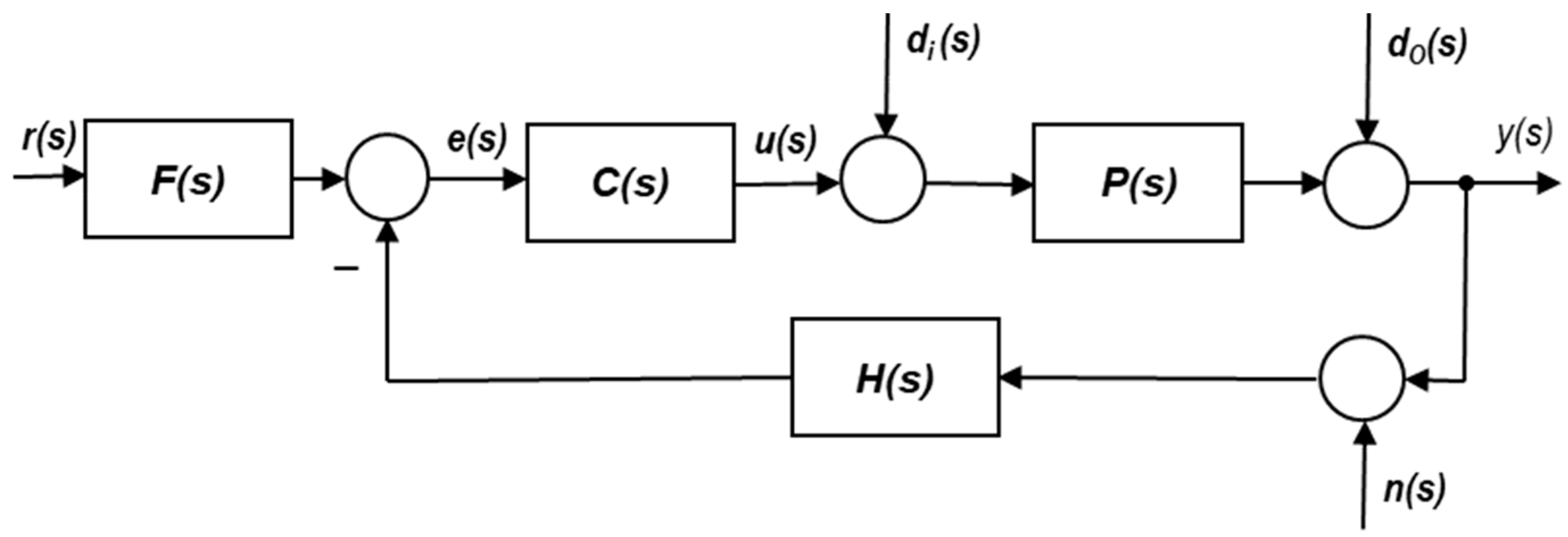
• Performance specifications.
  Stability and performance requirements are specified in terms of frequency-domain inequalities based on transfer functions between the inputs and outputs of a classical two-degree-of-freedom closed loop in Figure 2.
  $\left[\mathrm{r}\left(\mathrm{s}\right), \mathrm{n}\left(\mathrm{s}\right),{ \mathrm{d}}_{\mathrm{i}}\left(\mathrm{s}\right),{ \mathrm{d}}_0\left(\mathrm{s}\right)\right]$ are the inputs and $\left[ \mathrm{y}\left(\mathrm{s}\right),\mathrm{u}\left(\mathrm{s}\right), \mathrm{e}\left(\mathrm{s}\right)\right]$ are the outputs.
  Frequency-domain performance specifications have a general form:

  $$\left\{\left|{\mathrm{T}}_{\mathrm{k}}\left({\mathrm{j}\mathsf{\omega }}_{\mathrm{i}}\right)\right|\le {\mathsf{\delta }}_{\mathrm{k}}\left({\mathsf{\omega }}_{\mathrm{i}}\right),{ \mathsf{\omega }}_{\mathrm{i}}ϵ{\Omega }_{\mathrm{k}}, \mathrm{k}=1,2,\dots ; \mathrm{i}=1,2,\dots \right\}$$

  (25)

  where ${\mathrm{T}}_{\mathrm{k}}\left({\mathrm{j}\mathsf{\omega }}_{\mathrm{i}}\right)$ is the considered transfer function, ${\mathsf{\delta }}_{\mathrm{k}}\left({\mathsf{\omega }}_{\mathrm{i}}\right)$ is the upper limit of its magnitude, and ${\Omega }_{\mathrm{k}}$ is the set of frequencies from a selected range.
  The individual inequality specification types include:
  Type 1—Stability specification
  Type 2—Complementary sensitivity specification
  Type 3—Sensitivity or plant output disturbance specification
  Type 4—Plant input disturbance specification
  Type 5—Control action reduction specification
  Type 6—Reference tracking specification.
• Calculation of QFT bounds.
  Every plant in the ${\mathsf{\omega }}_{\mathrm{i}}$ template as well as the compensator can be expressed in their respective polar form:

  $$\begin{array}{c}\mathrm{P}\left({\mathrm{j}\mathsf{\omega }}_{\mathrm{i}}\right)={\mathrm{pe}}^{\mathrm{j}\mathsf{\theta }}=\mathrm{p}\angle \mathsf{\theta }\\ \mathrm{C}\left({\mathrm{j}\mathsf{\omega }}_{\mathrm{i}}\right)={\mathrm{ce}}^{\mathrm{j}\mathsf{\phi }}=\mathrm{c}\angle \mathsf{\phi }\end{array}$$

  (26)
  QFT bounds are calculated from the control specifications and consider model uncertainty. By substituting the polar forms (26) into individual selected performance specification types, they can be rearranged into quadratic inequalities in the form:

  $${\mathrm{l}}_{{\mathsf{\omega }}_{\mathrm{i}}}^{\mathrm{k}}\left(\mathrm{p},\mathsf{\varphi },{\mathsf{\delta }}_{\mathrm{k}},\mathsf{\theta }\right)={\mathrm{ac}}^2+\mathrm{bc}+\mathrm{f}\ge 0$$

  (27)

  where the coefficients $\mathrm{a},\mathrm{b},\mathrm{and} \mathrm{f}$ are functions of $\mathrm{p},\mathsf{\varphi },\mathsf{\theta },$ and ${\mathsf{\delta }}_{\mathrm{k}}$.
  Using an appropriate algorithm [20], the quadratic inequalities (27) are solved and translated into a set of curves in the Nichols diagram for each frequency and specification type. Thus, at each frequency ${\mathsf{\omega }}_{\mathrm{i}}$ and for each specification $\mathrm{k}$ there is a bound ${\mathrm{B}}_{\mathrm{k}}\left({\mathrm{j}\mathsf{\omega }}_{\mathrm{i}}\right)$ that can be dashed or solid, depending on whether the area satisfying the bound is above or below the line.
• Calculation of intersection by the QFT bounds and checking for their compatibility.
  If more than one performance specification is considered, it is necessary to find the intersection of all bounds at each frequency.
• Controller design by loop shaping in the Nichols diagram.
  After plotting the bounds in the Nichols diagram, it is sufficient to deal with just a single (nominal plant) to find a controller that meets the bounds. Hence, QFT provides an elegant and practical solution by integrating information associated with the model uncertainty and all control specifications in a set of simple curves. The loop-shaping design is carried out by adding poles and zeros until the nominal loop lies near its bounds (optimally on the top of the bounds at each frequency).
  The QFT compensator has a general form:

  $$\mathrm{C}\left(\mathrm{s}\right)={\mathrm{k}}_{\mathrm{C}}\frac{{\prod }_{\mathrm{i}=1}^{{\mathrm{n}}_{\mathrm{rz}}}\left(\left(\frac{\mathrm{s}}{{\mathrm{z}}_{\mathrm{i}}}\right)+1\right){\prod }_{\mathrm{i}=1}^{{\mathrm{n}}_{\mathrm{cz}}}\left(\left(\frac{{\mathrm{s}}^2}{{\mathsf{\omega }}_{\mathrm{ni}}^2}\right)+\left(\frac{2{\mathsf{\xi }}_{\mathrm{i}}}{{\mathsf{\omega }}_{\mathrm{ni}}}\right)\mathrm{s}+1\right)}{{\mathrm{s}}^{\mathrm{r}}{\prod }_{\mathrm{j}=1}^{{\mathrm{m}}_{\mathrm{rp}}}\left(\left(\frac{\mathrm{s}}{{\mathrm{p}}_{\mathrm{j}}}\right)+1\right){\prod }_{\mathrm{j}=1}^{{\mathrm{m}}_{\mathrm{cp}}}\left(\left(\frac{{\mathrm{s}}^2}{{\mathsf{\omega }}_{\mathrm{nj}}^2}\right)+\left(\frac{2{\mathsf{\xi }}_{\mathrm{j}}}{{\mathsf{\omega }}_{\mathrm{nj}}}\right)\mathrm{s}+1\right)},$$

  (28)

  where $\mathrm{z}$ denotes the zeros, $\mathrm{p}$ the poles, ${\mathsf{\omega }}_{\mathrm{n}}$ is the natural frequency, $\mathsf{\xi }$ is the relative damping, and ${\mathrm{k}}_{\mathrm{C}}$ is the gain.
• Prefilter design.
  A prefilter is used to solve the reference tracking problem.
• Analysis and validation.
  This step includes:

  -

  frequency domain analysis of each specification for all the significant plants within the model uncertainty,

  -

  time domain simulation for the linear and nonlinear systems.

To easily apply the QFT theory in practical tasks, a QFT Control Design Toolbox in MATLAB was developed in 1995 and has been continuously improved since [27,28,29]. In another commercially available version, the latest QFT techniques are implemented within a user-friendly and interactive environment [20].

4. Robust Decentralized QFT Controller Design Based on the Equivalent Subsystems Method

Development of the innovative robust decentralized controller design method based on the integration of the ESM and the QFT methods (ESM–QFT) is the main result of this article.

ESM provides the basic framework to implement the independent design of the local controllers for uncertain equivalent subsystems guaranteeing fulfillment of the necessary and sufficient stability conditions according to Theorem 2. Using the QFT method to independently design SISO controllers for the uncertain equivalent subsystems guarantees robust stability and required performance of the overall uncertain system. The theoretical background of the proposed ESM-QFT method evolved from the results provided in Theorem 2 and the QFT SISO design procedure described in Section 3.2 and is summarized in the following Lemma 1.

Lemma 1.

(Robust stability of a MIMO system under a decentralized controller). Consider the closed-loop in Figure 1, comprising the uncertain MIMO system and a decentralized controller, whereby the uncertain MIMO system consists of m subsystems and is denoted as a set (4) of square transfer function matrices (11) with an equal number of unstable poles $n_q$, and stable off-diagonal entries.

The closed-loop in Figure 1 is robustly stable if and only if for each transfer function matrix from the set (4) there exists $g_k^r\left(j\omega \right), r=1,\dots , N,$ such that $\forall s=j\omega \in \mathcal{D}$:

$$\begin{array}{c}1. \det \left[{\mathrm{g}}_{\mathrm{k}}^{\mathrm{r}}\left(\mathrm{j}\mathsf{\omega }\right)\mathrm{I}-{\mathrm{P}}_{\mathrm{n}}^{\mathrm{r}}\left(\mathrm{j}\mathsf{\omega }\right)\right]=0, \mathrm{k}\in \left\{1,2,\dots ,\mathrm{m}\right\}\\ 2. \sum _{i=1}^m\mathrm{N}\left\{-1,\left[{\mathrm{P}}_{\mathrm{ii}}^{\mathrm{r}}\left(\mathrm{j}\mathsf{\omega }\right)+{\mathrm{g}}_{\mathrm{k}}^{\mathrm{r}}\left(\mathrm{j}\mathsf{\omega }\right)\right]{\mathrm{C}}_{\mathrm{i}}\left(\mathrm{j}\mathsf{\omega }\right)\right\}={\mathrm{n}}_{\mathrm{q}}.\end{array}$$

(29)

Simply, for a selected $\mathrm{k}\in \left\{1,2,\dots ,\mathrm{m}\right\}$, the uncertain equivalent subsystems are the respective sets of mxN equivalent subsystems generated according to (21). Local robust SISO controllers are synthesized for each individual (i-th) uncertain equivalent subsystem independently using the QFT method; specifically, QFT templates are obtained by plotting ${\mathrm{P}}_{\mathrm{ik}}^{\mathrm{eq}\_\mathrm{r}}\left(\mathrm{j}\mathsf{\omega }\right)$ in the Nichols diagram of the i-th equivalent subsystem at each frequency ω of interest.

The ESM–QFT design procedure has the following steps:

I. 

Modeling the uncertain MIMO system

The uncertain MIMO system consisting of $\mathrm{m}$ interconnected subsystems can be given either as

• a set of $\mathrm{m}\times \mathrm{m}$ transfer matrices (4), or
• a single transfer matrix with entries having interrelated uncertain parameters.

In the latter case, the set of uncertain plant realizations is generated by gridding the uncertain parameters between their minimum and maximum values and considering all their (feasible) combinations. Then, $\mathrm{N}$ corresponds to the number of all feasible combinations of uncertain parameters.

One (any) of the realizations (4) can be chosen as a nominal system denoted as:

$${\mathrm{P}}^0\left(\mathrm{s}\right)=\left\{{\mathrm{P}}_{\mathrm{ij}}^0\left(\mathrm{s}\right)\right\}, \mathrm{i},\mathrm{j}=1,\dots , \mathrm{m}.$$

(30)

II. 

Generation of uncertain equivalent subsystems

Each transfer function matrix (5) from the set (4) can be split into the diagonal and off-diagonal transfer matrices ${\mathrm{P}}_{\mathrm{d}}^{\mathrm{r}}\left(\mathrm{s}\right)$ and ${\mathrm{P}}_{\mathrm{n}}^{\mathrm{r}}\left(\mathrm{s}\right)$, respectively:

$${\mathrm{P}}^{\mathrm{r}}\left(\mathrm{s}\right)={ \mathrm{P}}_{\mathrm{d}}^{\mathrm{r}}\left(\mathrm{s}\right)+{ \mathrm{P}}_{\mathrm{n}}^{\mathrm{r}}\left(\mathrm{s}\right), \mathrm{r}=1,\dots , \mathrm{N}.$$

(31)

For each ${\mathrm{P}}_{\mathrm{n}}^{\mathrm{r}}\left(\mathrm{s}\right), \mathrm{r}=1,\dots , \mathrm{N}$, the $\mathrm{m}$ characteristic functions are calculated as frequency-by-frequency, and the corresponding m sets per N characteristic loci ${\mathrm{g}}_{\mathrm{i}}^{\mathrm{r}}\left(\mathrm{j}\mathsf{\omega }\right), \mathrm{i}=1,\dots ,\mathrm{m};\mathrm{r}=1,\dots ,\mathrm{N}$ are plotted.

Using one selected $\left({\mathrm{k}}^{\mathrm{th}}\right)$ from the m sets of characteristic functions ${\mathrm{g}}_{\mathrm{k}}^{\mathrm{r}}\left(\mathrm{j}\mathsf{\omega }\right), \mathrm{k}\in \left\{1,\dots ,\mathrm{m}\right\};\mathrm{r}=1,\dots ,\mathrm{N}$; the respective sets per N equivalent subsystems are calculated according to (21) as follows:

$${\mathrm{P}}_{\mathrm{ik}}^{\mathrm{eq}\_\mathrm{r}}\left(\mathrm{j}\mathsf{\omega }\right)={\mathrm{P}}_{\mathrm{ii}}^{\mathrm{r}}\left(\mathrm{j}\mathsf{\omega }\right)+{\mathrm{g}}_{\mathrm{k}}^{\mathrm{r}}\left(\mathrm{j}\mathsf{\omega }\right), \mathrm{i}=1,2,\dots ,\mathrm{m}; \mathrm{k}\in \left\{1,2,\dots ,\mathrm{m}\right\}; \mathrm{r}=1,\dots ,\mathrm{N}.$$

(32)

III. 

Obtaining QFT templates

For one chosen $\mathrm{k}\in \left\{1,2,\dots ,\mathrm{m}\right\}$ and the respective sets of uncertain equivalent subsystems, QFT templates (32) are plotted in $\mathrm{m}$ Nichols diagrams.

IV. 

Independent design of SISO local controllers for uncertain equivalent subsystems

Independent design of local controllers for uncertain equivalent subsystems consists of m parallel designs according to steps 4–9 of the QFT design procedure in 3.2, including for each equivalent subsystem:

-

stability specification,

-

performance specification,

-

calculation of QFT bounds, their intersection and compatibility checking,

-

controller design by loop shaping of the chosen nominal equivalent subsystem in the Nichols diagram with the intersection of QFT bounds depicted.

V. 

Analysis of the frequency and time domains

The resulting decentralized controller $\mathrm{C}\left(\mathrm{s}\right)= \mathrm{diag} \left\{{\mathrm{C}}_{\mathrm{i}}\left(\mathrm{s}\right)\right\}, \mathrm{i}=1,\dots ,\mathrm{m}$ is a diagonal matrix composed of the individual local controllers designed for the respective uncertain equivalent subsystems.

Frequency-domain analysis is carried out at the equivalent subsystem levels and includes the verification of the required stability performance specifications.

Time-domain analysis relates to the overall system level when the decentralized controller is implemented in the real subsystems; it is based on simulations for linear/nonlinear models under various simulation scenarios.

5. Case Study

The proposed design method was verified on a benchmark case study dealing with the design of a robust decentralized level control in a quadruple tank process [8,17,23]. The freely available toolbox [27,28,30] with the necessary modifications performed was used to perform the independent QFT designs for the uncertain equivalent subsystems.

5.1. Description of the Controlled Plant

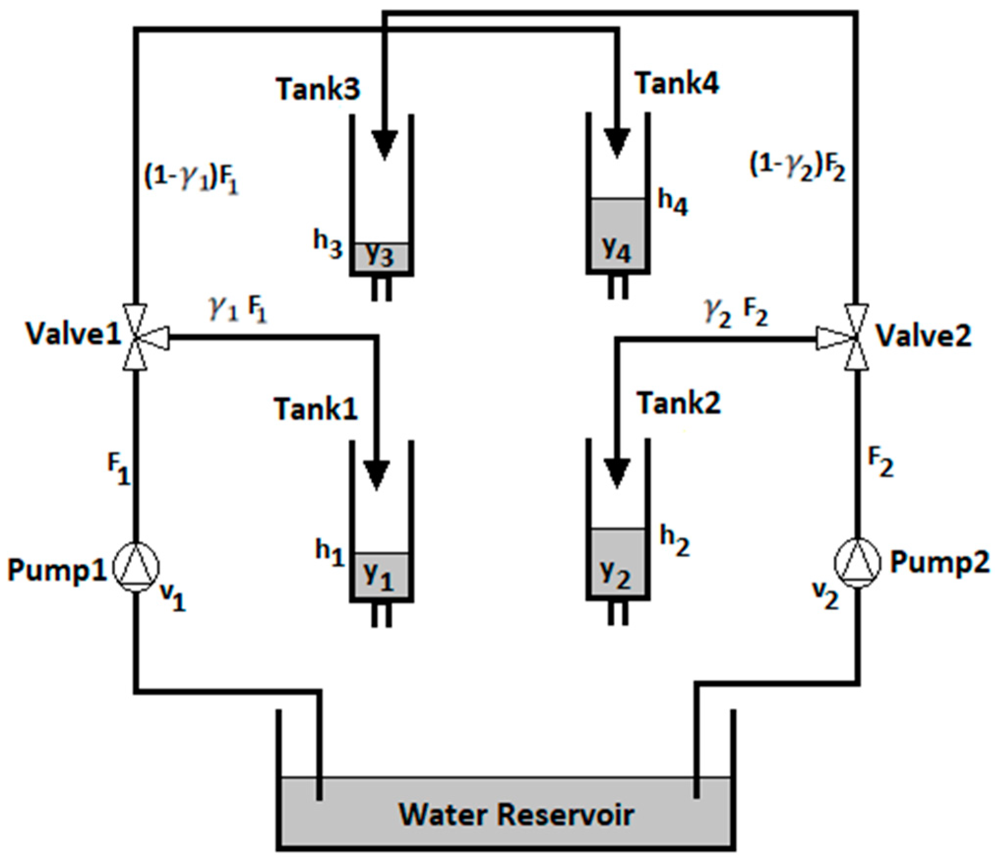
The quadruple-tank process (Figure 3) is a laboratory plant, which is suitable to analyze and demonstrate different approaches to control a two-input two-output MIMO system in either the minimum and/or nonminimum phase configurations [23].

Level control in the two lower tanks is performed using two pumps, with their voltages ${\mathrm{v}}_1,$ ${\mathrm{v}}_2 \left[\mathrm{V}\right]$ as the inputs. The levels in the lower tanks ${\mathrm{h}}_1$,${\mathrm{h}}_2 \left[\mathrm{cm}\right]$ are the controlled outputs. The pump voltages define the corresponding inflows ${\mathrm{F}}_{\mathrm{i}}={\mathrm{k}}_{\mathrm{i}}{\mathrm{v}}_{\mathrm{i}}, \mathrm{i}=1,2$. The parameters ${\mathsf{\gamma }}_{\mathrm{i}}, \mathrm{i}=1,2$ denote the valve settings, i.e., relative ratios of pump flows into the lower and upper diagonal tanks (tanks 1 and 4 for ${\mathsf{\gamma }}_1,$ and tanks 2 and 3 for ${\mathsf{\gamma }}_2$), hence, ${\mathsf{\gamma }}_{1 },{ \mathsf{\gamma }}_2 ϵ〈0,1〉$.

The first principles nonlinear state space model of the device has the form:

$$\begin{array}{l}\frac{{\mathrm{dh}}_1}{\mathrm{dt}}=-\frac{{\mathrm{a}}_1}{{\mathrm{A}}_1}\sqrt{2{\mathrm{gh}}_1}+\frac{{\mathrm{a}}_3}{{\mathrm{A}}_1}\sqrt{2{\mathrm{gh}}_3}+\frac{{\mathsf{\gamma }}_{1 }{\mathrm{k}}_{1 }}{{\mathrm{A}}_1}{\mathrm{v}}_1\\ \frac{{\mathrm{dh}}_2}{\mathrm{dt}}=-\frac{{\mathrm{a}}_2}{{\mathrm{A}}_2}\sqrt{2{\mathrm{gh}}_2}+\frac{{\mathrm{a}}_4}{{\mathrm{A}}_2}\sqrt{2{\mathrm{gh}}_4}+\frac{{\mathsf{\gamma }}_{2 }{\mathrm{k}}_2}{{\mathrm{A}}_2}{\mathrm{v}}_2\\ \frac{{\mathrm{dh}}_3}{\mathrm{dt}}=-\frac{{\mathrm{a}}_3}{{\mathrm{A}}_3}\sqrt{2{\mathrm{gh}}_3}+\frac{\left(1-{\mathsf{\gamma }}_2\right){\mathrm{k}}_2}{{\mathrm{A}}_3}{ \mathrm{v}}_2\\ \frac{{\mathrm{dh}}_4}{\mathrm{dt}}=-\frac{{\mathrm{a}}_4}{{\mathrm{A}}_4}\sqrt{2{\mathrm{gh}}_4}+\frac{\left(1-{\mathsf{\gamma }}_1\right){\mathrm{k}}_1}{{\mathrm{A}}_4}{ \mathrm{v}}_1,\end{array}$$

(33)

where ${\mathrm{A}}_{\mathrm{i}}$ and ${\mathrm{a}}_{\mathrm{i}}, \mathrm{i}=1,\dots , 4$ are cross-sections of individual tanks and of their outlet holes, respectively; ${\mathrm{h}}_{\mathrm{i}}, \mathrm{i}=1,\dots , 4$ are levels in individual tanks; g is the gravitational acceleration.

The plant model can be configured as either a minimum or nonminimum phase depending on the relative ratios of the pump flows ${\mathsf{\gamma }}_{1, }{\mathsf{\gamma }}_2.$

For the minimum-phase configuration, the following condition is satisfied:

$$1<{\mathsf{\gamma }}_1+{\mathsf{\gamma }}_2<2,$$

(34)

and the nonminimum-phase condition is:

$$0<{\mathsf{\gamma }}_1+{\mathsf{\gamma }}_2<1.$$

(35)

By linearization of (33) around a selected working point specified by the levels in the individual tanks ${\mathrm{h}}_{\mathrm{i}0},\mathrm{i}=1,\dots ,$4, the corresponding transfer function matrix is obtained [23]:

$$\mathrm{P}\left(\mathrm{s}\right)=\left[\begin{array}{cc}\frac{{\mathrm{c}}_{1 }{\mathsf{\gamma }}_{1 }}{{\mathrm{T}}_{1 }\mathrm{s}+1}& \frac{{\mathrm{c}}_1\left(1-{\mathsf{\gamma }}_{2 }\right)}{({\mathrm{T}}_{3 }\mathrm{s}+1)\left({\mathrm{T}}_{1 }\mathrm{s}+1\right)}\\ \frac{{\mathrm{c}}_2\left(1-{\mathsf{\gamma }}_{1 }\right)}{({\mathrm{T}}_{4 }\mathrm{s}+1)\left({\mathrm{T}}_{2 }\mathrm{s}+1\right)}& \frac{{\mathrm{c}}_{2 }{\mathsf{\gamma }}_{2 }}{{\mathrm{T}}_{2 }\mathrm{s}+1}\end{array}\right]$$

(36)

where

$${\mathrm{T}}_{\mathrm{i}}=\frac{{\mathrm{A}}_{\mathrm{i}}}{{\mathrm{a}}_{\mathrm{i}}}\sqrt{\frac{2{\mathrm{h}}_{\mathrm{i}}^0}{\mathrm{g}}}, \mathrm{i}=1,\dots ,4 { \mathrm{c}}_{\mathrm{i}}=\frac{{\mathrm{T}}_{\mathrm{i}}{\mathrm{k}}_{\mathrm{i}}{\mathrm{k}}_{\mathrm{c}}}{{\mathrm{A}}_{\mathrm{i}}}\sqrt{\frac{2{\mathrm{h}}_{\mathrm{i}}^0}{\mathrm{g}}}, \mathrm{i}=1,2$$

(37)

The values of the individual plant parameters were taken from [8] and are shown in

Table 1. Parameter values for the quadruple tank process.

Parameter	${\mathbf{A}}_1, {\mathbf{A}}_3$ $\left[\mathbf{c}{\mathbf{m}}^2\right]$	${\mathbf{A}}_2, {\mathbf{A}}_4$ $\left[\mathbf{c}{\mathbf{m}}^2\right]$	${\mathbf{a}}_1, {\mathbf{a}}_3$ $\left[\mathbf{c}{\mathbf{m}}^2\right]$	${\mathbf{a}}_2, {\mathbf{a}}_4$ $\left[\mathbf{c}{\mathbf{m}}^2\right]$	${\mathbf{h}}_1^0, {\mathbf{h}}_2^0$ $\left[\mathbf{c}\mathbf{m}\right]$	${\mathbf{h}}_3^0$ $\left[\mathbf{c}\mathbf{m}\right]$	${\mathbf{h}}_4^0$ $\left[\mathbf{c}\mathbf{m}\right]$	${\mathbf{k}}_{\mathbf{c}}$	${\mathbf{k}}_{1 }$	${\mathbf{k}}_{2 }$	$\mathbf{g}$ $\left[\mathbf{c}\mathbf{m}/{\mathbf{s}}^2\right]$
Value	30	35	0.0977	0.079	20	2.75	2.22	1	1.79	1.827	981

.

5.2. Control Problem Statement

For the quadruple tank system, the aim is to control the levels in the two lower tanks (h₁, h₂) by means of the flows delivered by the two pumps (v₁, v₂) in the operating range, specified by the valve settings (${\mathsf{\gamma }}_{1 },$ ${\mathsf{\gamma }}_{2 }$) which represent uncertain parameters that are interrelated depending on the specific plant configurations (34) or (35). Hence, the plant has $\mathrm{m}=2$ subsystems, the minimum phase configuration is considered and the decentralized control structure is employed.

5.3. Robust Decentralized Controller Design

The ESM–QFT design procedure described in Section 4 was used to design the robust decentralized controller.

I. 

Modeling the uncertain MIMO system

The linearized model for the uncertain plant based on parameter values in Table 1 is:

$$\mathrm{P}\left(\mathrm{s}\right)=\left[\begin{array}{cc}\frac{0.747{\mathsf{\gamma }}_{1 }}{62.044\mathrm{s}+1}& \frac{0.747\left(1-{\mathsf{\gamma }}_{2 }\right)}{\left(22.992\mathrm{s}+1\right)\left(62.044\mathrm{s}+1\right)}\\ \frac{0.949\left(1-{\mathsf{\gamma }}_{1 }\right)}{\left(29.995\mathrm{s}+1\right)\left(90.031\mathrm{s}+1\right)}& \frac{0.949{\mathsf{\gamma }}_{2 }}{90.031\mathrm{s}+1}\end{array}\right].$$

(38)

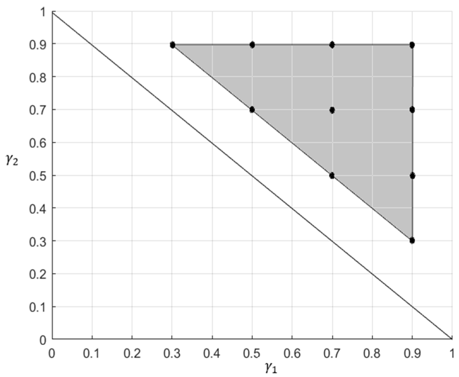
When considering the minimum phase plant configuration, the two uncertain parameters ${\mathsf{\gamma }}_{1 },$ ${\mathsf{\gamma }}_{2 }\in 〈0, 1〉$ are interrelated according to (34). The set of realizations of the uncertain plant was generated by gridding ${\mathsf{\gamma }}_{1 },$ ${\mathsf{\gamma }}_{2 }\in 〈0.3, 0.9〉$ and considers all their combinations that meet (33). The number of feasible combinations is $\mathrm{N}=10$. The corresponding combinations specifying the considered uncertainty region are depicted in Figure 4. The nominal model was selected as (38) evaluated in ${\mathsf{\gamma }}_1=$ ${\mathsf{\gamma }}_{2 }=0.7.$

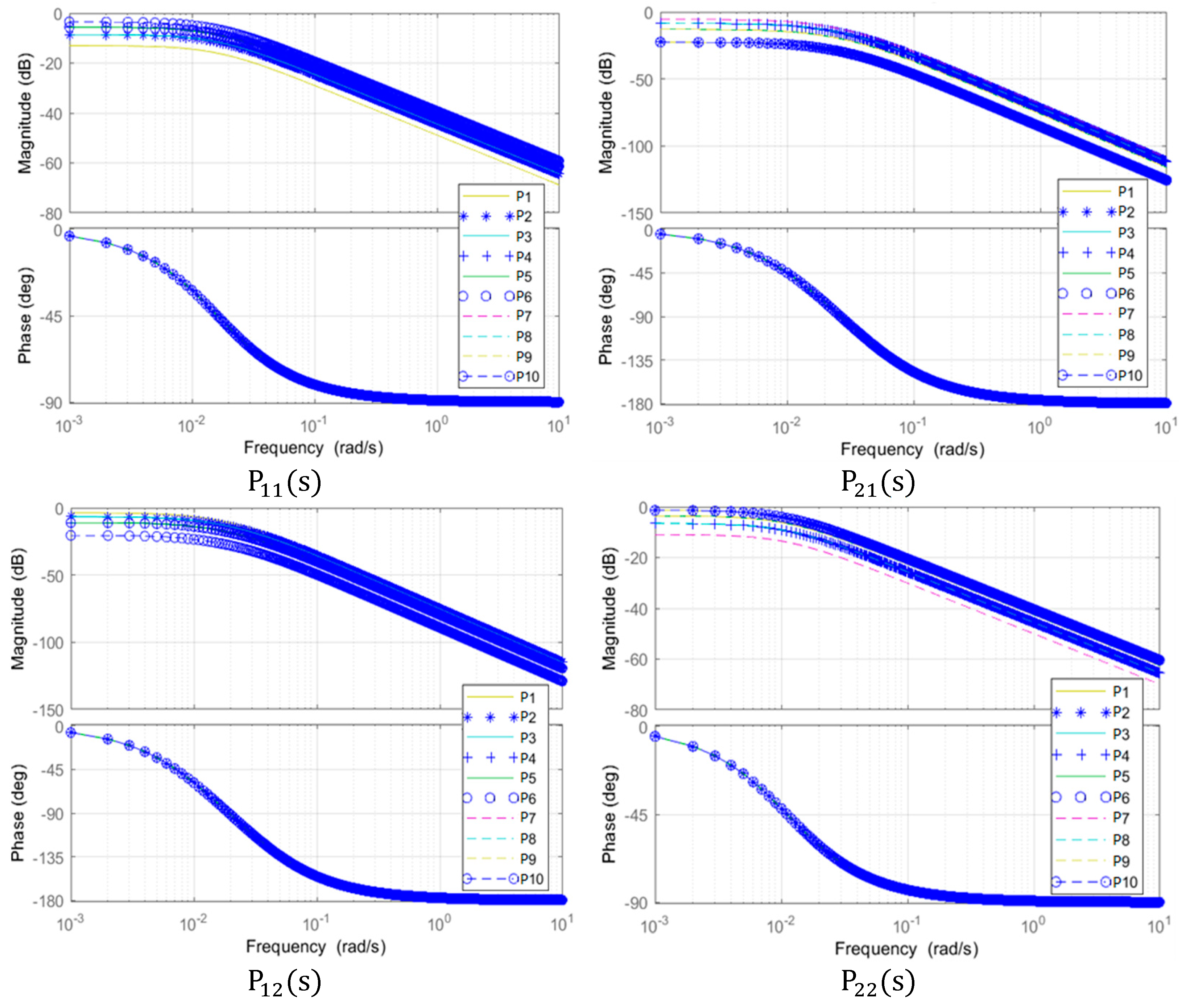
To appropriately choose the frequency range for the controller design, the Bode diagrams of the individual entries of (38), considering the settings in

Table 2. Plant realizations according to valve settings (34).

	1	2	3	4	5	6	7	8	9	10
${\mathsf{\gamma }}_1$	0.3	0.5	0.5	0.7	0.7	0.7	0.9	0.9	0.9	0.9
${\mathsf{\gamma }}_2$	0.9	0.9	0.7	0.5	0.7	0.9	0.3	0.5	0.7	0.9

, are depicted in Figure 5.

II. 

Generation of uncertain equivalent subsystems

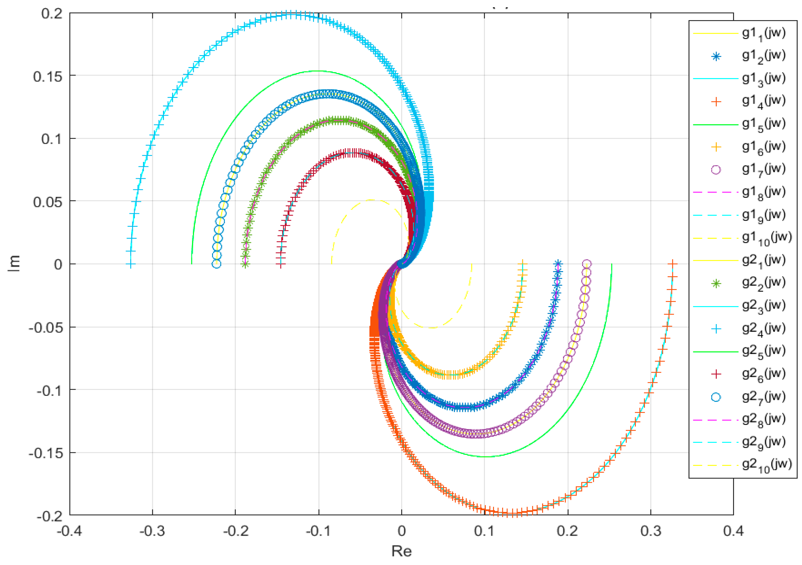
Characteristic loci of the matrices of interactions ${\mathrm{P}}_{\mathrm{n}}^{\mathrm{r}}\left(\mathrm{s}\right), \mathrm{r}=1,\dots 10$ are depicted in Figure 6.

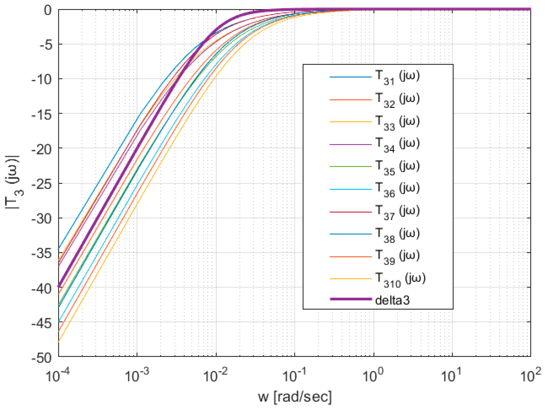
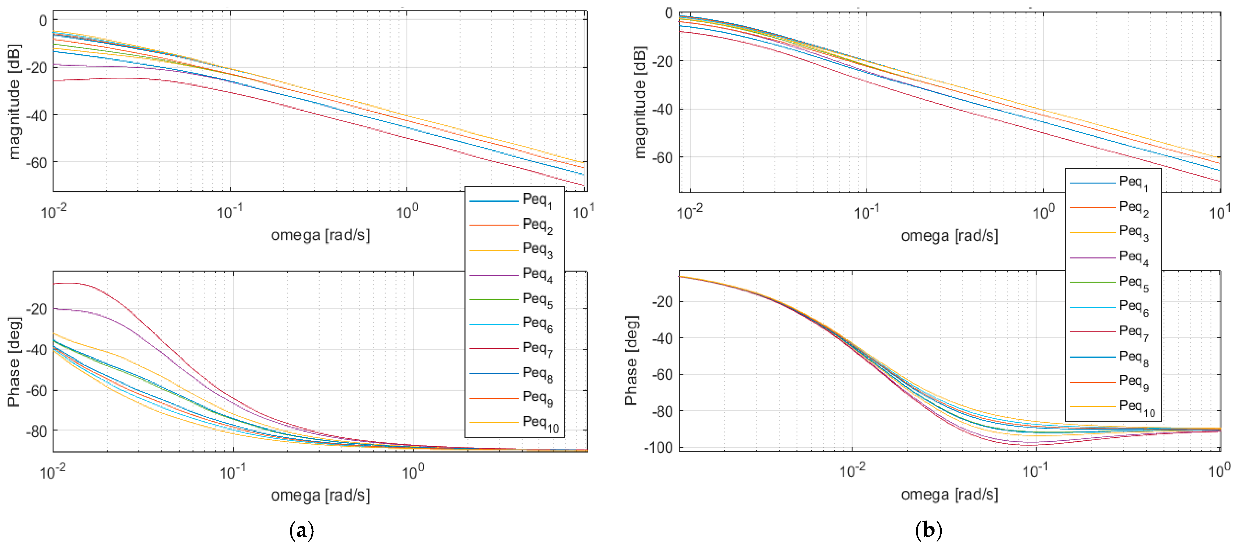
Equivalent subsystems are generated according to (21) using the respective characteristic loci ${\mathrm{g}}_2^{\mathrm{r}}\left(\mathrm{j}\mathsf{\omega }\right),\mathrm{r}=1,\dots ,10$:

$${\mathrm{P}}_{\mathrm{i}2}^{\mathrm{eq}\_\mathrm{r}}\left(\mathrm{j}\mathsf{\omega }\right)={\mathrm{P}}_{\mathrm{ii}}^{\mathrm{r}}\left(\mathrm{j}\mathsf{\omega }\right)+{\mathrm{g}}_2^{\mathrm{r}}\left(\mathrm{j}\mathsf{\omega }\right), \mathrm{i}=1,2; \mathrm{r}=\left\{1,2,\dots ,10\right\},$$

(39)

with the respective Bode diagrams shown in Figure 7.

III. 

Obtaining QFT templates of uncertain equivalent subsystems

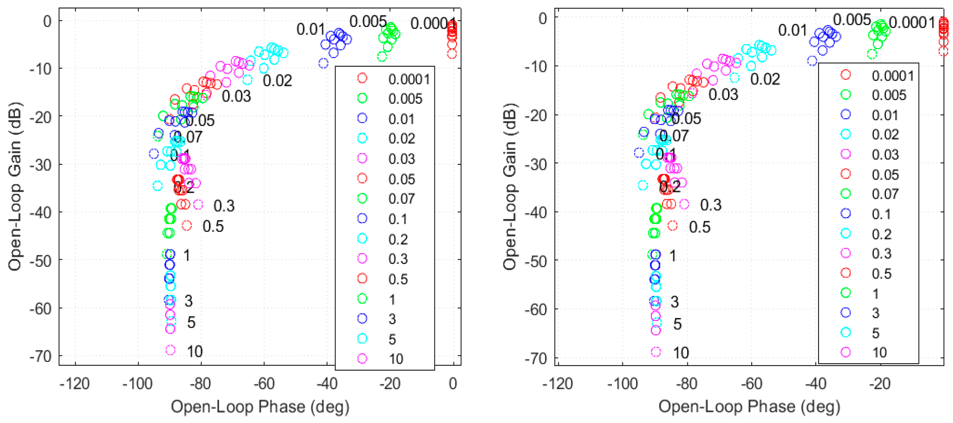
For the set of uncertain equivalent subsystems (39), corresponding QFT templates were plotted in the Nichols diagrams (Figure 8) for the selected frequencies $\mathsf{\omega }=\left\{0.0001 0.005 0.01 0.02 0.03 0.05 0.07 0.01 0.2 0.3 0.5 1 3 5 10\right\}.$

IV. 

Independent design of SISO local controllers${\mathrm{C}}_{\mathrm{i}}\left(\mathrm{s}\right)=1,2$for uncertain equivalent subsystems

Time-domain performance requirements for the overall system usually specified in terms of time-domain measurements (maximum overshoot, settling time) had to be interpreted into frequency domain measures; two out of eight following QFT stability and performance specifications [20] similar for both equivalent subsystems were selected:

• Stability specification (determines 20% maximum overshoot of output responses):

  $$\left|{\mathrm{T}}_1\left(\mathrm{j}\mathsf{\omega }\right)\right|=\left|\frac{{\mathrm{P}}_{\mathrm{i}2}^{\mathrm{eq}\_\mathrm{r}}\left(\mathrm{j}\mathsf{\omega }\right){\mathrm{C}}_i\left(\mathrm{j}\mathsf{\omega }\right)}{1+{\mathrm{P}}_{\mathrm{i}2}^{\mathrm{eq}\_\mathrm{r}}\left(\mathrm{j}\mathsf{\omega }\right){\mathrm{C}}_i\left(\mathrm{j}\mathsf{\omega }\right)}\right|\le {\mathrm{W}}_{\mathrm{si}}=1.2, \mathrm{i}=1,2.$$

  (40)
• Performance specification (sensitivity constraint) determines bandwidth, which is a measure of the speed of response, similar to time domain measures, such as rise time or peak time [31]:

  $$\left|{\mathrm{T}}_3\left(\mathrm{j}\mathsf{\omega }\right)\right|=\left|\frac{1}{1+{\mathrm{P}}_{\mathrm{i}2}^{\mathrm{eq}\_\mathrm{r}}\left(\mathrm{j}\mathsf{\omega }\right){\mathrm{C}}_{\mathrm{i}}\left(\mathrm{j}\mathsf{\omega }\right)}\right|\le {\mathsf{\delta }}_{3\mathrm{i}}=\frac{\left(\mathrm{s}/{\mathrm{a}}_{\mathrm{di}}\right)}{\left(\mathrm{s}/{\mathrm{a}}_{\mathrm{di}}\right)+1}, \mathrm{i}=1,2$$

  (41)

  where ${\mathrm{a}}_{\mathrm{di}}=0.01, \mathrm{i}=1,2$.

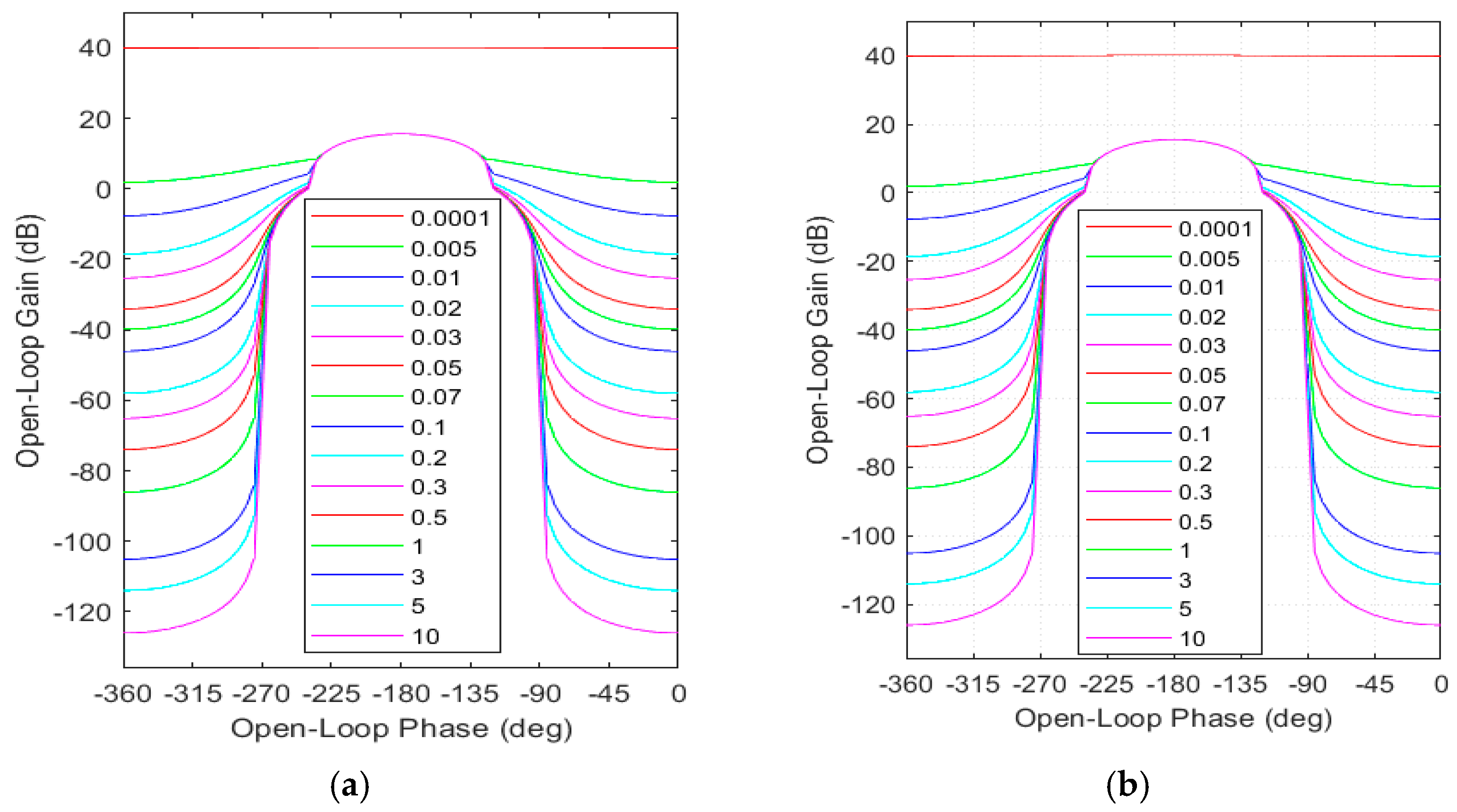
Based on performance specifications and QFT templates, the QFT bounds were calculated and their intersections were plotted in the Nichols diagrams (Figure 9).

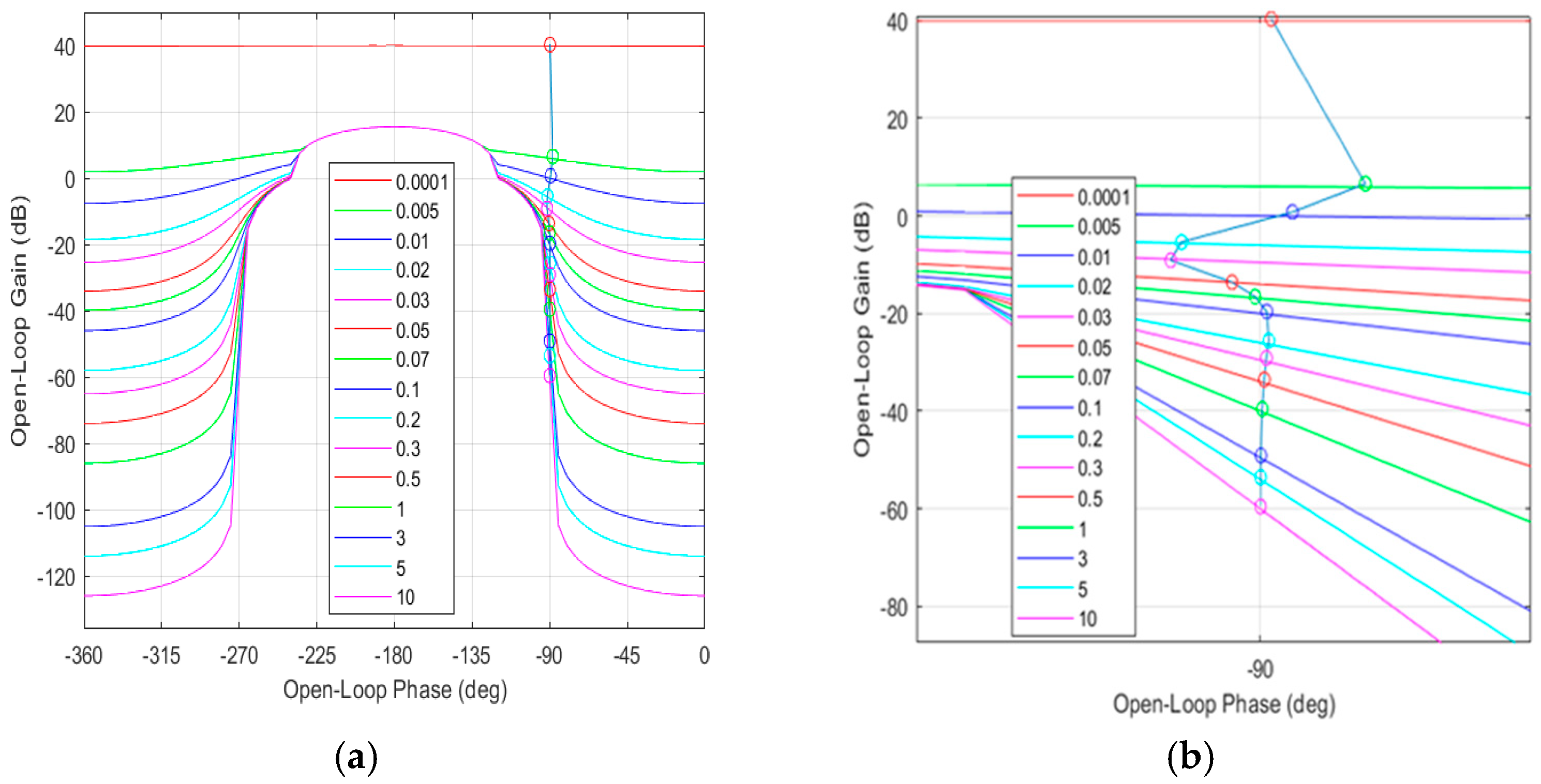
Local controllers ${\mathrm{C}}_{\mathrm{i}}\left(\mathrm{s}\right)=1,2$ were designed by loop shaping of nominal open loops ${\mathrm{L}}_{0\mathrm{i}}\left(\mathrm{j}\mathsf{\omega }\right)={\mathrm{P}}_{\mathrm{i}2}^{\mathrm{eq}\_5}\left(\mathrm{j}\mathsf{\omega }\right){\mathrm{C}}_{\mathrm{i}}\left(\mathrm{j}\mathsf{\omega }\right), \mathrm{i}=1,2$, in the respective Nichols diagrams with depicted QFT bounds (Figure 10 and Figure 11).

Local controllers designed for equivalent subsystems constitute the resulting decentralized controller to be implemented for the real system:

$$\mathrm{C}\left(\mathrm{s}\right)=\left[\begin{array}{cc}{\mathrm{C}}_1\left(\mathrm{s}\right)& 0\\ 0& {\mathrm{C}}_2\left(\mathrm{s}\right)\end{array}\right]=\left[\begin{array}{cc}1.2485+\frac{0.0384}{\mathrm{s}}& 0\\ 0& 1.4582+\frac{0.04487 }{\mathrm{s}}\end{array}\right],$$

(42)

V. 

Analysis of the frequency and time domains

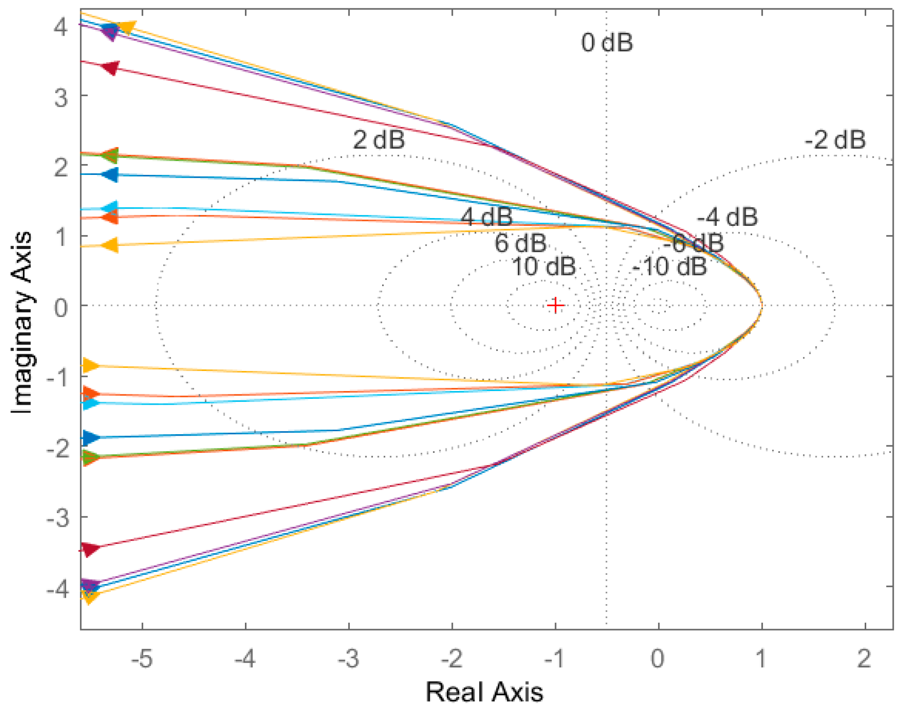
Frequency domain analysis includes:

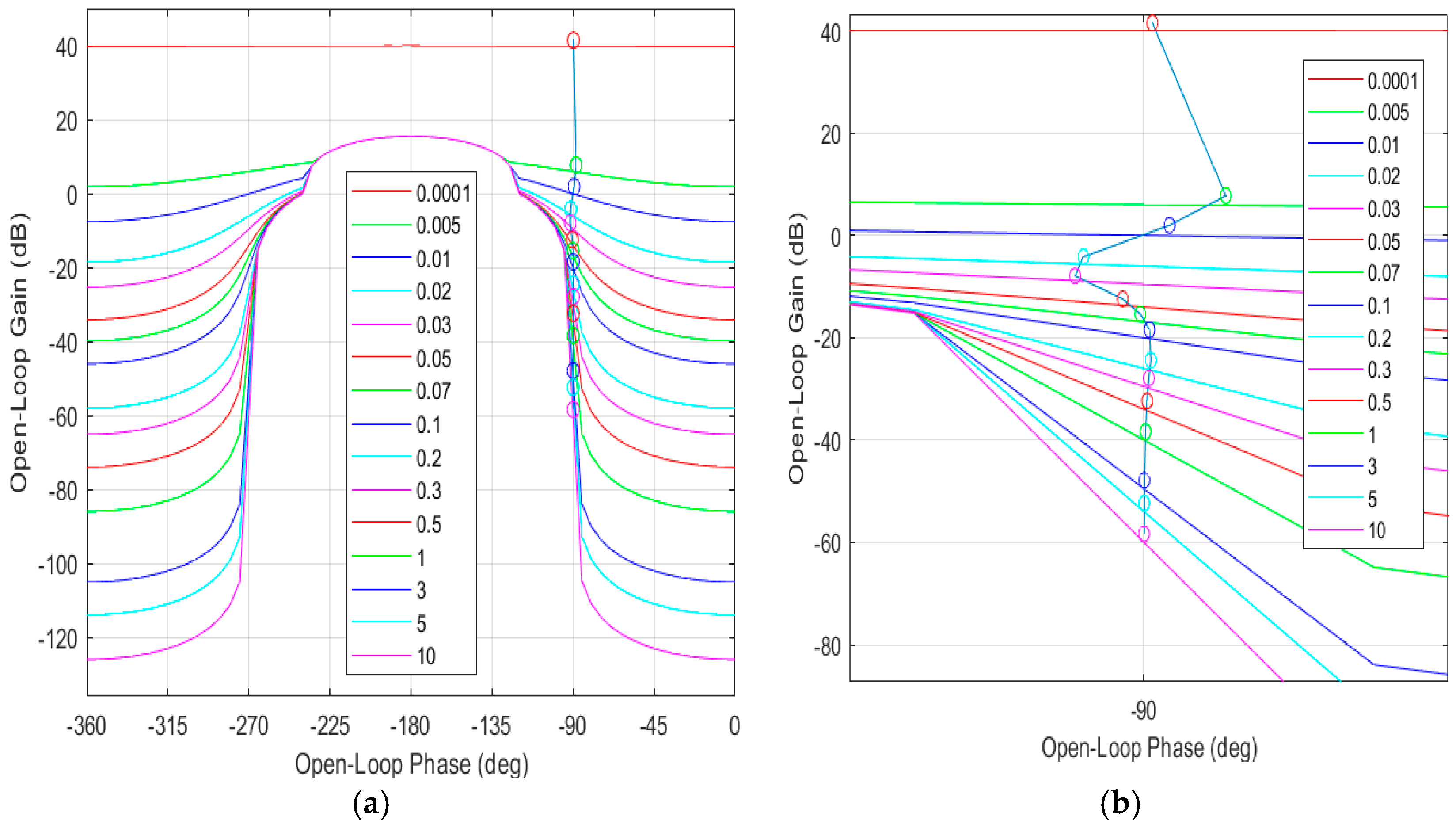
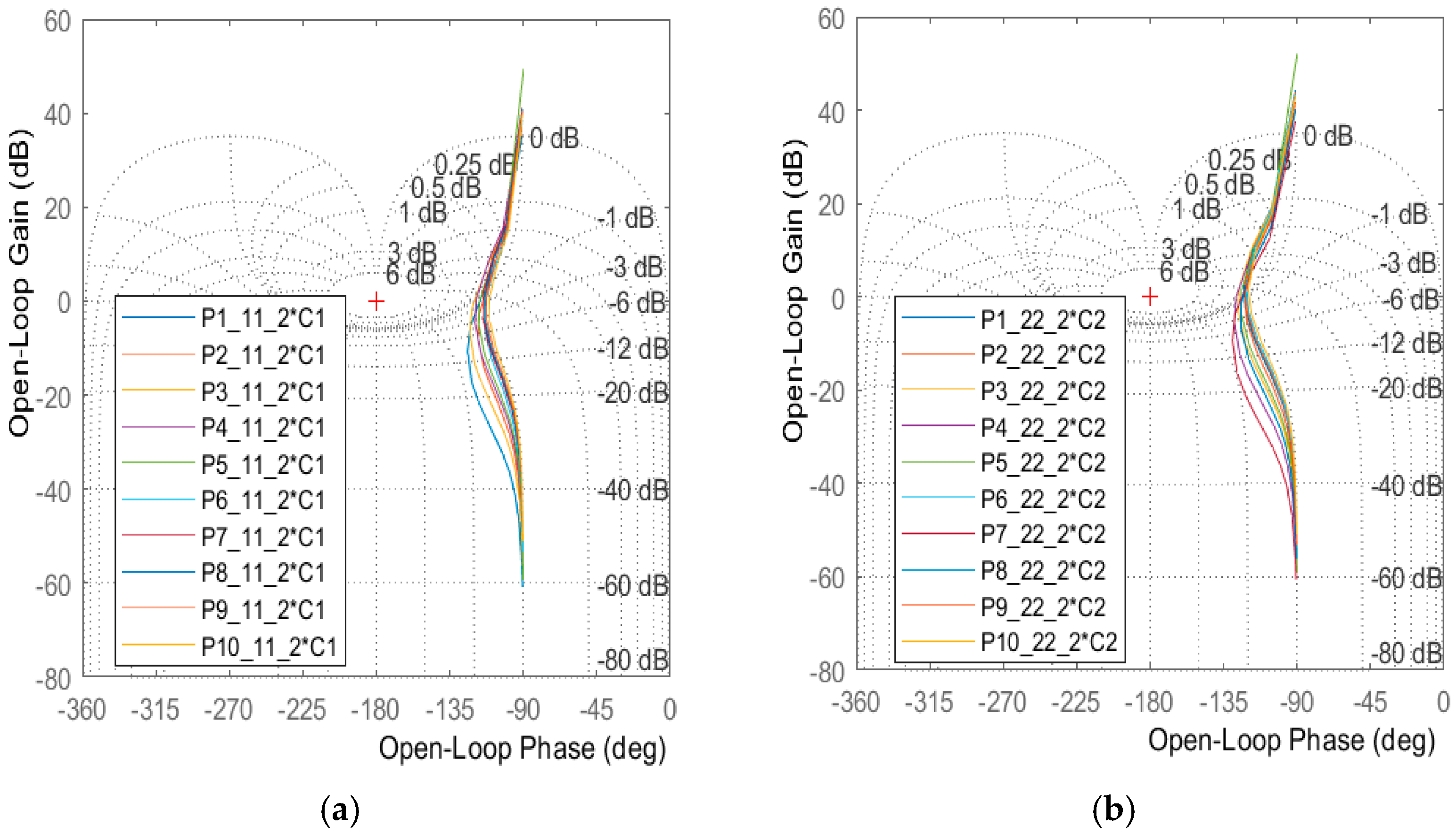
• verification of the fulfillment of the performance requirements in the equivalent subsystems by plotting Nichols plots of open-loop equivalent subsystems ${\mathrm{P}}_{\mathrm{i}2}^{\mathrm{eq}\_\mathrm{r}}\left(\mathrm{j}\mathsf{\omega }\right){\mathrm{C}}_{\mathrm{i}}\left(\mathrm{j}\mathsf{\omega }\right), \mathrm{i}=1,2$ for r = 1, …,10 to (Figure 12),
• investigation of the fulfillment of the performance requirements for the overall closed-loop system by plotting the spectral norm of sensitivity of the overall system under the decentralized controller (Figure 13),
• closed-loop stability verification using the generalized Nyquist stability criterion (2) (Figure 14).

For both equivalent subsystems, Nichols diagrams in Figure 12 prove stability and fulfillment of the Type 1 specification (40) since neither of the depicted Nichols plots intersects or touches the curve of the value $20\log \left(1.2\right)=1.58 \mathrm{dB}$ corresponding to ${\mathrm{W}}_{\mathrm{s}}=1.2$.

The required minimum bandwidth specified for the equivalent subsystems by the Type 3 performance specification (41) is kept for all realizations of the overall system (Figure 13, ${\mathsf{\delta }}_3\left(\mathsf{\omega }\right)$ is depicted in bold), the minimum bandwidth achieved is ${\mathsf{\omega }}_{\mathrm{BW}}=0.008 {\mathrm{s}}^{-1}$.

The overall closed-loop system under the decentralized controller (42) is stable as $\mathrm{N}\left[0,\det \left[\mathrm{I}+\mathrm{Q}\left(\mathrm{s}\right)\right]\right]={\mathrm{n}}_{\mathrm{q}}=0$ for all 10 plant realizations considered (Figure 14).

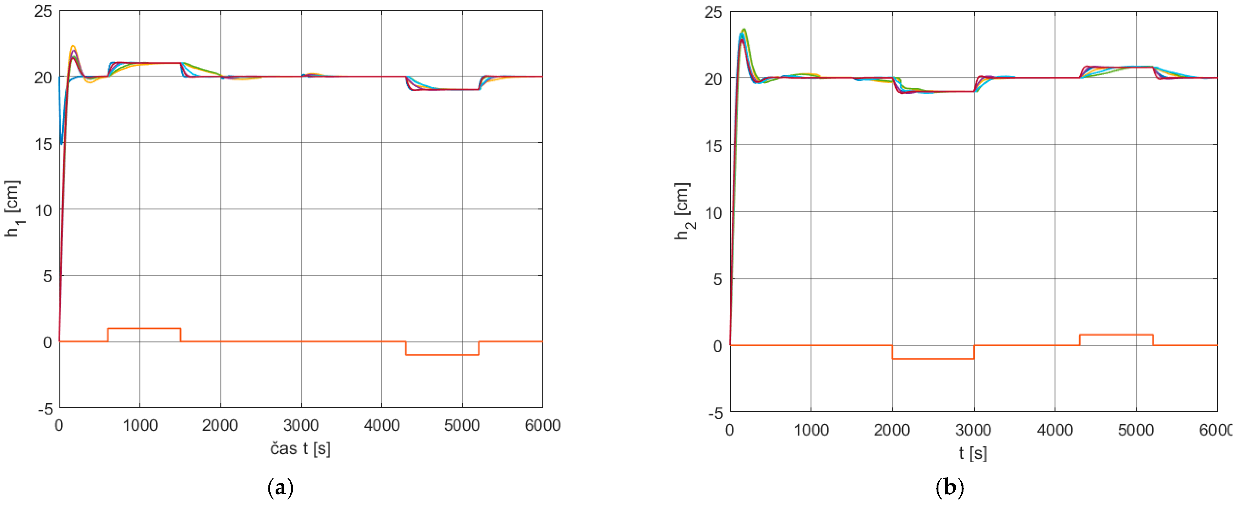
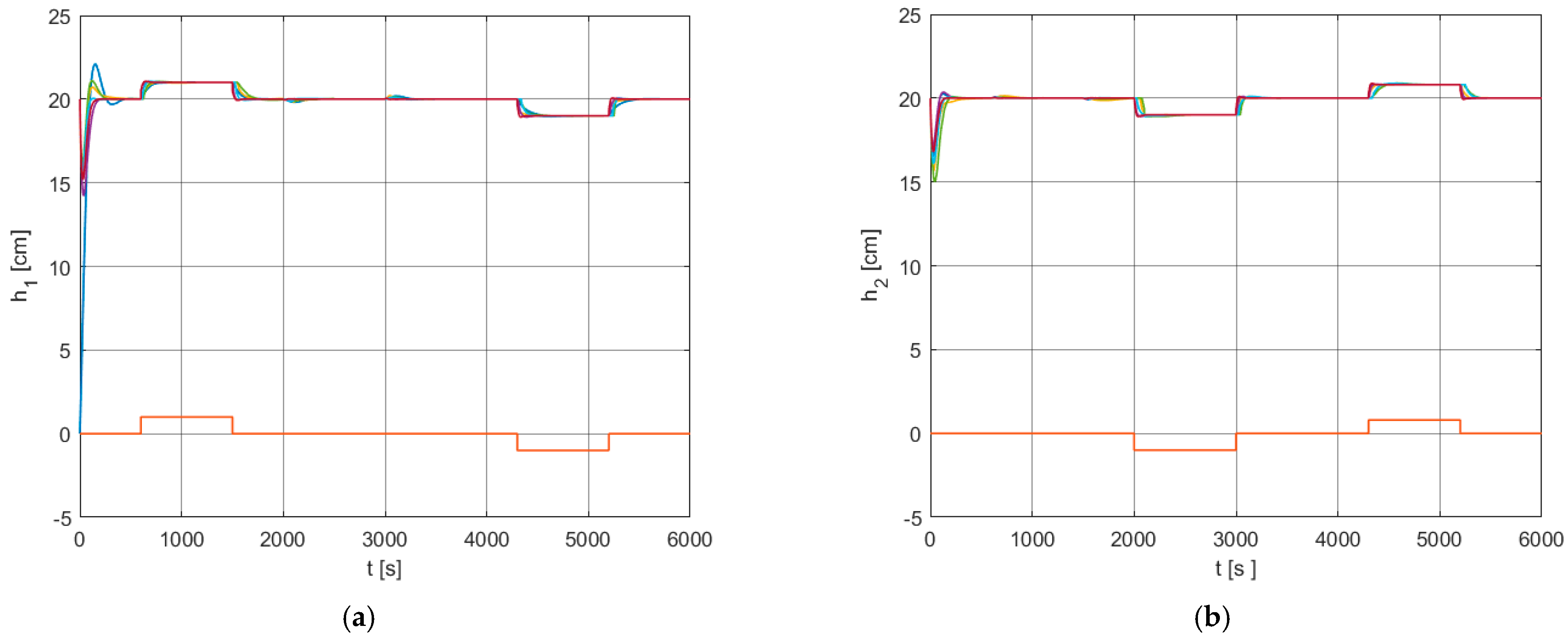
Time domain analysis is based on simulations of step changes in references of the lower tanks according to scenarios depicted in the lower parts of the charts in Figure 15 and Figure 16. Simulations were performed using both the linear and the nonlinear models (36) and (33), respectively, in the specified working point ${\mathrm{h}}_{\mathrm{i}}^0, \mathrm{i}=1, \dots , 4$ for all 10 valve settings ${\mathsf{\gamma }}_1,$ ${\mathsf{\gamma }}_{2 }$, according to Table 2. Respective output responses are depicted in Figure 15 (linear model) and Figure 16 (nonlinear model); the performance on individual charts is of interest only after the variables have first settled at the respective working points.

Responses in Figure 15 and Figure 16 are another proof of the fulfillment of the Type 1 specification (39), as the overshoots of the responses ${\mathrm{h}}_1\left(\mathrm{t}\right)$ a ${\mathrm{h}}_2\left(\mathrm{t}\right)$ are ${\mathsf{\eta }}_{\max }<20\%$.

6. Discussion

The proposed ESM–QFT is a frequency domain method that is suitable for designing robust decentralized controllers for uncertain MIMO systems with an equal number of input and output variables, which consist of interconnected SISO subsystems and are given as a set of square transfer function matrices with an equal number of unstable poles and stable off-diagonal entries. The synergetic integration of ESM and the standard QFT SISO design allows the assets of both methods to be exploited.

Using the ESM, local controllers are designed for individual equivalent subsystems independently and subsequently implemented into true subsystems as a decentralized controller, thereby guaranteeing the fulfillment of the necessary and sufficient stability conditions, in the sense of the generalized Nyquist stability theorem. Compared to standard independent designs, which consider the diagonal system as the nominal one e.g., [6], the robust ESM-based methods deal with the full nominal system being transformed into a set of equivalent subsystems. Moreover, using uncertain equivalent subsystems avoids the need to consider an unnecessarily broad uncertainty domain due to unstructured uncertainty modeling when integrating the general robust stability condition in local designs [17]. Hence, the conservatism of the design is reduced considerably.

The design of local SISO controllers for individual equivalent subsystems can be performed using any SISO frequency domain method. However, the independent design based on QFT is advantageous in that the uncertain equivalent subsystems generated directly from the transfer matrices of the uncertain MIMO system are directly QFT templates. Performance requirements imposed on the overall uncertain system are usually specified in the time domain; the ESM–QFT method guarantees their fulfillment if they are translated into the frequency domain performance specifications fulfilled in the individual uncertain equivalent subsystems.

The ESM–QFT method uses nonparametric models of the controlled system and related frequency dependencies; hence, the design procedure is graphical, insightful, and interactive, and may be applied for continuous and discrete, minimum- and non-minimum phase systems as well as for systems with delays.

Finally, the proposed ESM–QFT is a unique general and simple-to-use robust decentralized controller design method based on independent designs. Future research will encompass the application of the developed method for the various types of MIMO systems and case studies.