Research on Propagation Characteristics Based on Channel Measurements and Simulations in a Typical Open Indoor Environment

Abstract

At present, it is difficult to obtain the indoor propagation loss quickly and accurately by directly using measurements in the millimeter wave band. To solve this problem, in this paper, a ray tracing method suitable for indoor scenes based on geometric optics theory, the uniform theory of diffraction and image theory is presented; the space-alternation generalized expectation-maximization (SAGE) algorithm is used to analyze the measured data and the multipath information of the wireless channel is analyzed; three deep learning models are used to predict the path loss at different receiving distances based on 1600 sets of path loss data. The results show that the comparison between the ray tracing and experimental results shows a good agreement. Moreover, the root-mean-square error (RMSE) and mean absolute error (MAE) of the long short-term memory (LSTM) network are the smallest, and the LSTM has a better fitting effect on the propagation loss sequences predicted at more distant locations when compared with the recurrent neural network (RNN) and gate recurrent unit (GRU) methods, which can better reflect the propagation trend. This provides theoretical support for the layout of base stations and network optimization in typical open indoor environments.

1. Introduction

With the huge demand for data services brought about by mobile internet and the Internet of Things, spectrum resources are gradually becoming saturated. However, the abundant spectrum resources available in the millimeter wave can effectively alleviate the tension of spectrum resources and meet the needs of fifth-generation (5G) mobile communication systems [1,2,3] in terms of high capacity, high speed transmission and low delay. Therefore, millimeter wave-based 5G communication technology is one of the most promising technologies for fifth-generation wireless mobile communication systems.

Because 5G millimeter wave communication has the characteristics of a close propagation distance and high attenuation and is greatly influenced by meteorological fluctuations, the development of large outdoor scenarios for 5G millimeter wave communication has great difficulties of long propagation distance, complex atmospheric environment and rich scenes. However, indoor scenes are the main production and living scenes of human beings and have the characteristics of limited propagation distance, small mobile interference and negligible meteorological fluctuations. The indoor wireless propagation environment is ideally suited to avoid the characteristic shortcomings of the 5G millimeter wave [4,5]. Therefore, studying a 5G millimeter wave indoor channel propagation model has an important meaning in scientific research and practicality for the promotion and application of millimeter wave technology, as well as the next technical direction for the study of outdoor millimeter waves. The typical open indoor office environment (as seen in Figure 1) has transitioned from a small-space partitioned office environment to a large-space open office environment to improve office efficiency. Since typical open indoor environments [6] mainly use low-frequency electromagnetic waves with slow transmission rates and narrow bandwidths, poor network speeds and unstable connections of indoor communication signals are common. This scenario cannot meet the demands of current centralized office networks. However, the millimeter wave can effectively improve the signal transmission rate and communications density. Consequently, there is an urgent need to research the wireless channel propagation characteristics of millimeter waves in a typical open indoor environment.

It is necessary to conduct research on wireless channel modeling to ensure the accuracy and reliability of a wireless propagation model. The main methods involve both measurements and computer simulations. Measurements can directly reflect the electromagnetic characteristics of a scenario and accurately assess the field performance, but they require significant labor and time costs. In contrast, computer simulations can also evaluate the electromagnetic properties of specific scenarios to obtain more accurate predictions and significantly reduce the time and labor costs. Computer simulations can be optimized through extensive computer simulations and measurements. The ray tracing method [7,8,9,10], which is widely used in indoor and outdoor wireless channel propagation, is an effective means to conduct research on channel models in the millimeter wave. The ray tracing method can better assess the problem of electromagnetic wave propagation and is widely used in the channel modeling of millimeter waves. There is little literature on the fast and accurate acquisition of propagation loss at all points indoors in the millimeter wave band. In 1991, Lawton M C et al. [11] predicted a power delay profile based on the three-dimensional shooting and bouncing of rays in a room environment. In 1998, Steven Fortune [12] used geometric optics-based ray tracing and beam tracing methods to compare the time required for ray tracing and beam tracing methods in the same scene, as well as the mean difference, standard deviation and maximum difference calculated for different ray intervals. In 2003, R. Hoppe et al. proposed an accelerated ray-optical model. Based on a single preprocessing of a database, the mutual visibility relationship between walls and building edges was determined [13]. In 2013, V. Degli-Esposti et al. proposed a simple two-parameter indoor path loss formulation that takes into account the main propagation mechanism in indoor environments and compares it with indoor experiments at 858 MHz and 1935 MHz [14]. In 2017, Wallace J W et al. [15] compared the link gain, path loss, channel capacity and root-mean-square delay spread for two university buildings consisting of classrooms and offices in parallel 4 × 4 multiple-input multiple-output measurements at 2.55 GHz and 24 GHz, respectively. In 2018, Geok T K et al. [16] introduced the maximum accuracy method for indoor 3D minimum ray emission, which can significantly reduce the number of rays to be tracked, and compared the coverage, the number of emitted rays, the number of received rays and the simulation time. Moreover, in the same year, Danping He et al. provided a comprehensive overview of the design and application of ray tracing methods [17]. In 2019, Chen Y S et al. [18] analyzed the radiation characteristics of antennas used for indoor Wi-Fi based on the shooting and bouncing ray and the image method and proposed design guidelines to enhance the received power. In the same year, Hossain F et al. [19] proposed an effective three-dimensional ray tracing method to study indoor radio wave propagation at 28 GHz, and their results showed that the simulation software based on the effective three-dimensional ray tracing method was in good agreement with the test data. In 2020, H. Obeidat et al. introduced various deterministic channel modeling methods, such as the finite integral method, finite difference time domain, dominant path model and ray tracing method [20]. In 2020, Ubaid Ullah et al. provide a ray tracing method for 5G millimeter wave outdoor-to-indoor and indoor-to-indoor scenarios [21].

The framework for this study is as follows. In Section 1, the three-dimensional ray tracing method for indoor scenes and the SAGE algorithm are introduced. In Section 2, channel measurement experiments are described in office and conference room scenarios. Section 3 analyzes the wireless channel parameters for office and conference room scenarios and predicts the path loss at different distances using three deep learning models. In Section 4, a summary is presented.

2. Theory

2.1. Ray Tracing Method

The three-dimensional ray tracing method determines the ray path when the locations of the transmitting antenna, receiving antenna and obstacles are known. This method is useful in situations where there are relatively few objects and obstacles, such as typical open indoor environments. The three-dimensional ray tracing method is more accurate than other methods, and it can determine all the rays from the transmitter to the receiver. Moreover, it has a fast computing speed. Since the inner walls are relatively smooth in an office, the scattering effect does not need to be considered. However, the line of sight, specular reflection and transmission need to be considered. In this paper, a ray tracing method suitable for a typical open indoor environment is presented to determine the effective reflection path and transmission path between the transmitting and receiving antennas by considering the line of sight, reflection and transmission and to calculate the electric field and the power from the transmitting antenna to the receiving antenna by combining the radiation pattern. The ray tracing method in this paper is programmed and implemented independently, which can be controlled independently.

The specific steps for implementing the three-dimensional reverse ray tracing method in a typical open indoor environment are as follows.

First, the relevant parameters needed in the simulation are set, including the operating frequency, position coordinates, polarization mode and transmission power of the transmitting antenna; the position coordinates and polarization mode of the receiving antenna; the radiation pattern of the transmitting and receiving antennas; and the height of the ceiling.

Second, the environmental information and electromagnetic parameters in typical open indoor environments are loaded. Buildings such as walls, floors and ceilings are described, and the locations of objects such as desks and cabinets are also described in typical open indoor environments. The specific environmental information is the position coordinates of the buildings and the building numbers; the electromagnetic parameters contain the dielectric permittivity and conductivity of the materials, which are provided in reference [2,22]. The electromagnetic parameters of various materials are very different, and the different electromagnetic parameters have a great effect on the predicted electric fields.

Next, the core step of the propagation prediction model is to determine the effective ray path between the transmitting and receiving antennas based on the information of a typical open indoor environment, which has a great impact on the simulation efficiency. This includes the direct path, single reflection/transmission path and double reflections/transmission path from the transmitting to receiving antennas. The pseudocode for determining the electric field caused by direct rays between transmitting and receiving antennas (all combinations of line of sight and transmissions with a maximum number of one transmission) is shown in Algorithm 1. The point of the single reflection is found according to the image method, whether transmission occurs is determined and the single reflection/transmission path between the transmitting and receiving antennas is finally determined. Moreover, transmission is directly considered in the calculation of single reflection. The pseudocode for determining the electric field caused by single reflection/transmission (all combinations of single reflection and transmissions with a maximum number of one transmission) between transmitting and receiving antennas is shown in Algorithm 2. Similarly, the point of the double reflections is determined according to the image method, whether transmission occurs is determined and the double reflection/transmission (all combinations of double reflections and transmissions with a maximum number of two transmissions) path between the transmitting and receiving antennas is finally determined.

Algorithm 1 Determine the Electric Field caused by direct ray between Transmitter and Receiver

1: procedure Electric field E

2:   m          ▷The connection ray between the transmitter and receiver

3:   tt, cc        ▷intersection, walls

4:      for cc do

5:    tt ← Determine if the ray m has an intersection tt with an wall cc

6:        if The intersection is on the wall then

7:           T ← Calculation transmission coefficient between the transmitter and receiver

8:        else

9:           T = 1

10:         end if

11:      end for 12:     E ← Calculate the electric field caused by direct ray/transmission 13:     return E

14: end procedure

Algorithm 2 Determine the Electric Field caused by single reflection/transmission path between Transmitter and Receiver

1: procedure Electric field E1

2:    m            ▷The connection ray between single image point and receiver 3:    m1             ▷The connection ray between transmitter and reflection point 4:    m2             ▷The connection ray between reflection point and receiver 5:    tt, cc             ▷Intersection of single image point and receiver with walls, walls 6:    tt1              ▷Intersection of transmitter and reflection point with walls 7:    tt2              ▷Intersection of receiver and reflection point with walls

8:     for cc do 9:       R             ▷reflection coefficient between transmitter and receiver

10:     tt ← Determine if the ray m has an intersection tt with walls cc

11:      if The intersection is on the wall then

12:        R ← Calculation of reflection coefficient R according to Fresnel’s Formula

13:          for cc do

14:            tt1 ← Determine if the ray m1 has an intersection tt1 with walls cc 15:             if The intersection is on the wall then 16:                T1 ← Calculate transmission coefficient between transmitter and reflection point 17:             else 18:                T1 = 1 19:             end if 20:          end for 21:          for cc do 22:             tt2 ← Determine if the ray m2 has an intersection tt2 with walls cc 23:             if The intersection is on the wall then 24:                T2 ← Calculate transmission coefficient between reflection point and receiver 25:             else 26:                T2 = 1 27:             end if 28:          end for 29:             E11 ← Calculate the electric field caused by each path

30:       end if

31:    end for 32:    E1 ← Calculate the total electric field caused by single reflection/transmission 33:    return E1

34: end procedure

Then, the electric field and the received power are calculated for each effective ray path. Finally, the total electric fields of all the rays are superimposed at each receiving antenna.

2.2. SAGE Algorithm

The SAGE algorithm has been widely used for wireless channel parameter estimation. The SAGE algorithm consists of two steps: the E-step and the M-step.

A more detailed theory and implementation of the SAGE algorithm can be found in the literature [23,24,25]. In this paper, the SAGE algorithm is used to estimate the multipath signal parameters, including the time delay, arrival angle, departure angle, Doppler shift and amplitude. For a single-input multiple-output system, the receiving antenna consists of an antenna array that consists of M antennas located at different locations. The received signal can be represented as

$$Y(t)={\displaystyle \sum _{l=1}^{L}s(t;{\theta }_l)}+\sqrt{N_0/2}N(t)$$

(1)

where $N(t)$ is Gaussian white noise and $s(t;{\theta }_l)$ is the received signal of the $l$-th path, which can be expressed as

$$s(t;{\theta }_l)\triangleq [s_1(t,{\theta }_l),\dots ,s_{M_2}(t,{\theta }_l)]=C({\Omega }_l){\alpha }_l\exp (j2\pi {\nu }_{l}t)u(\tau -{\tau }_l)$$

(2)

where ${\theta }_l=[{\tau }_l,{\Omega }_l,{\nu }_l,{\alpha }_l]$ is the vector of the $l$-th multipath parameter, which is the time delay, arrival angle, Doppler shift and amplitude of the multipath. Since the measurements are stationary, the Doppler shift is not considered in the SAGE algorithm. $u(\tau -{\tau }_l)$ is the transmitted signal. The M-dimensional vector function consisting of the unit vector $\Omega$ is $C(\Omega )\triangleq {[c_1(\Omega ),c_2(\Omega ),c_3(\Omega ),\dots ,c_M(\Omega )]}^T$, which is shown as

$$c_m(\Omega )\triangleq f_m(\Omega )\exp (j2\pi {\nu }_{l}t{\lambda }^{-1}<e(\Omega ),r_m>),m=1,\dots ,M$$

(3)

where $\lambda$ is the wavelength, $e(\Omega )={[\cos \varphi \sin \theta ,\sin \varphi \sin \theta ,\cos \theta ]}^T$, is the spherical coordinate unit vector determined by $\Omega$, and $f_m(\Omega )$ is the complex weight of the m-th antenna element, $r_m$ is the position receiving antenna array element. The dot product $<e(\Omega ),r_m>$ is expressed as

$$<e(\Omega ),r_m>=[x_m-d_x,y_m-d_y,z_m-d_z]\cdot {[\cos \varphi \sin \theta ,\sin \varphi \sin \theta ,\cos \theta ]}^T$$

(4)

where $[x_m,y_m,z_m]$ are the relative position coordinates of the m-th array element, $d_x$, $d_y$, $d_z$ are the antenna array element spacings of the X/Y/Z axes, respectively.

2.2.1. Signal Model in Translational Scanning System

In the measurement, the transmitter and receiver both use horn antennas, as shown in Figure 2. The transmitting antenna is fixed, and the horn antenna is moved M and N times along the horizontal and vertical directions, respectively, to form a virtual antenna array. Since the measurements are time invariant, the Doppler shift is not considered in the SAGE algorithm. $u(t-{\tau }_l)$ is the transmitted signal. The channel impulse response of the $l$-th path can be expressed as

$$s(t;{\rho }_l)\doteq {[s_1(t;{\rho }_l),s_2(t;{\rho }_l),\dots ,s_N(t;{\rho }_l)]}^T={\alpha }_l\exp \left\{i2\pi {\nu }_{l}t\right\}c(\theta ,\phi )u(t-{\tau }_l)$$

(5)

where ${\rho }_l=[{\tau }_l,{\theta }_l,{\phi }_l,{\nu }_l,{\alpha }_l]$ is the set of parameters to be found. ${\tau }_l$ is the time delay of the $l$-th path, ${\theta }_l$ is the vertical angle of arrival of the $l$-th path, ${\phi }_l$ is the horizontal angle of arrival of the $l$-th path, ${\nu }_l$ is the Doppler shift of the $l$-th path, ${\alpha }_l$ is the amplitude of the $l$-th path, and $c(\theta ,\phi )$ is the steering vector, which can be expressed as

$$c(\theta ,\phi )=\left[\begin{array}{c}{c}_1(\theta ,\phi )\\ .\\ .\\ .\\ c_M(\theta ,\phi )\end{array}\right]=\left[\begin{array}{c}{f}_1(\theta ,\phi )\exp (i2\pi /\lambda <e(\theta ,\phi ),r_1>)\\ .\\ .\\ .\\ f_M(\theta ,\phi )\exp (i2\pi /\lambda <e(\theta ,\phi ),r_M>)\end{array}\right]$$

(6)

where $r_M$ is the position of the M-th array element of the receiving antenna array, $f_M(\theta ,\phi )$ is the complex weight of the M-th array element of the receiving antenna array and $e(\theta ,\phi )$ is the unit vector.

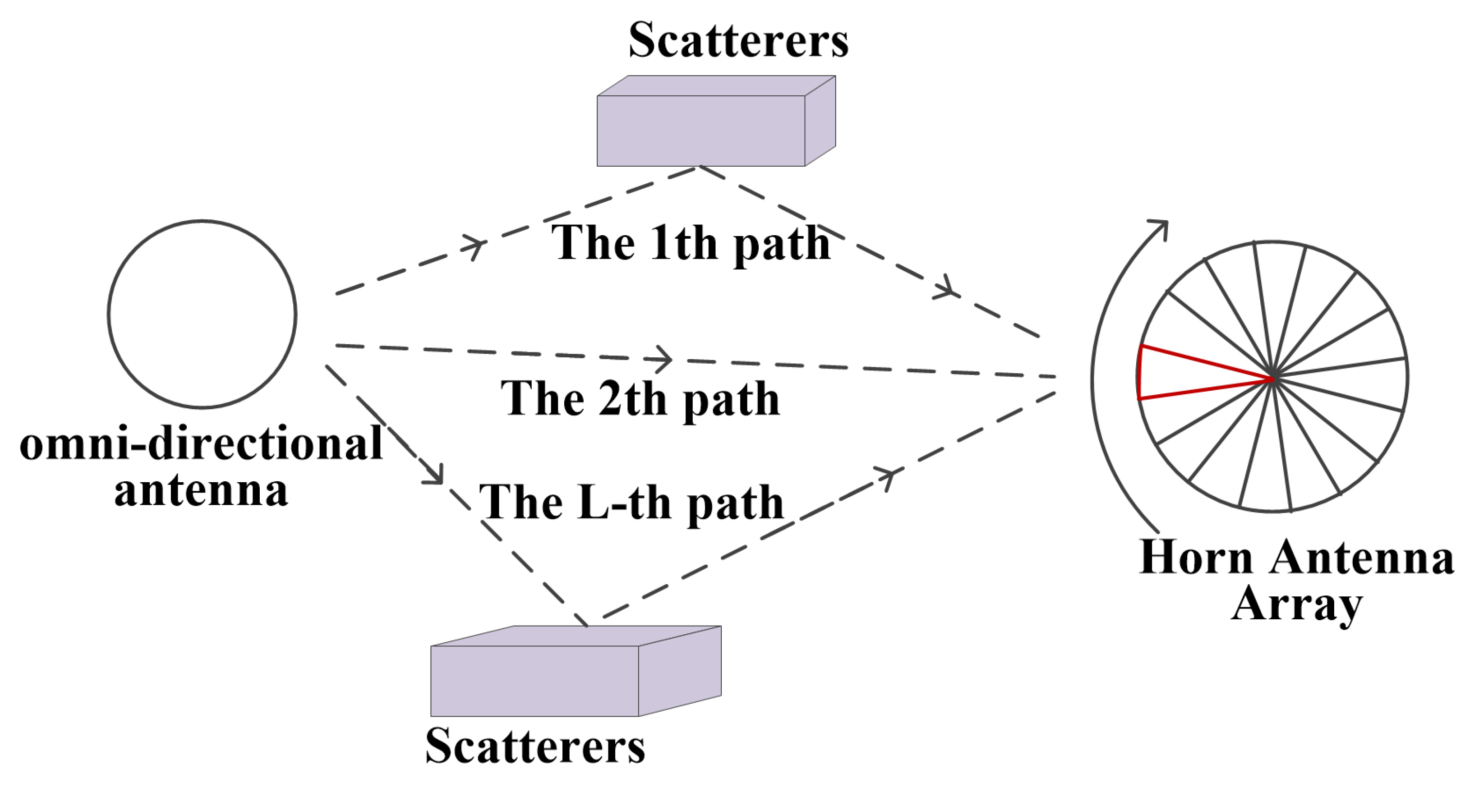
2.2.2. Signal Model in Rotary Scanning System

In this section, an omnidirectional antenna is used at the transmitter, and a horn antenna is used at the receiver in the measurement, as shown in Figure 3. The virtual antenna array is constructed by fixing the omnidirectional antenna and rotating the horn antenna N times. The Doppler shift is not considered in the SAGE algorithm. The channel impulse response of the $l$-th multipath is

$$s(t;{\rho }_l)={\alpha }_{l}c(\theta ,\phi )u(t-{\tau }_l)$$

(7)

where ${\rho }_l=[{\tau }_l,{\theta }_l,{\phi }_l,{\nu }_l,{\alpha }_l]$. When the horn antenna is rotated, the feed point is always in one position, so $c(\theta ,\phi )$ can be simplified as

$$c(\theta ,\phi )=\left[\begin{array}{c}{f}_1(\theta -{\theta }_1,\phi -{\phi }_1)\\ .\\ .\\ .\\ f_M(\theta -{\theta }_1,\phi -{\phi }_1)\end{array}\right]$$

(8)

2.3. Deep Learning Models and Performance Assessment Metrics

A recurrent neural network (RNN) extracts features with the help of loop kernels and sends them into subsequent networks, such as the fully connected network Dense, for prediction [26,27]. The RNN extracts information from the temporal dimension with the help of loop kernels, and the parameters of the loop kernel are shared in time [19]. The loop kernel has memory and enables the extraction of information from a time series by sharing parameters at different moments.

Long short-term memory (LSTM) was proposed by Hochreiter and Schmidhuber in 1997 [28,29,30], and it provides a good solution to the long-term dependency problem of the RNN by gating the unit. The LSTM can solve the long-term dependency problem of RNNs because LSTM uses the gate mechanism to control the flow and loss of information. Three gates are introduced in LSTM, including the input gate, forget gate and output gate, as well as memory cells with the same shape as the hidden state. Thus, it can record additional information.

Compared with LSTM, the unit structure of a gate recurrent unit (GRU) is simple [31]; the GRU reduces and merges the gate structure of LSTM to only reset and update gates, which increases the speed of network training and ensures accuracy.

To evaluate the predictive performance of deep learning models, the mean squared error (RMSE) and mean absolute error (MAE) are used to evaluate the predictive performance of the deep learning models based on the test set. The smaller the RMSE and MSE are, the better the predictive performance of the deep learning models. The RMSE and MSE are defined, respectively, as

$$RMSE=\sqrt{\frac{{\displaystyle {\sum }_{\mathrm{i}=1}^N{(P{L}^{pred}(i)-PL(i))}^2}}{N}}$$

(9)

$$MAE=\frac{{\displaystyle {\sum }_{\mathrm{i}=1}^N|P{L}^{pred}(i)-PL(i)|}}{N}$$

(10)

where $P{L}^{pred}(i)$ denotes the predicted i-th value of path loss sequence, $PL(i)$ represents the actual i-th value calculated by ray tracing and $N$ is the total number of the test set.

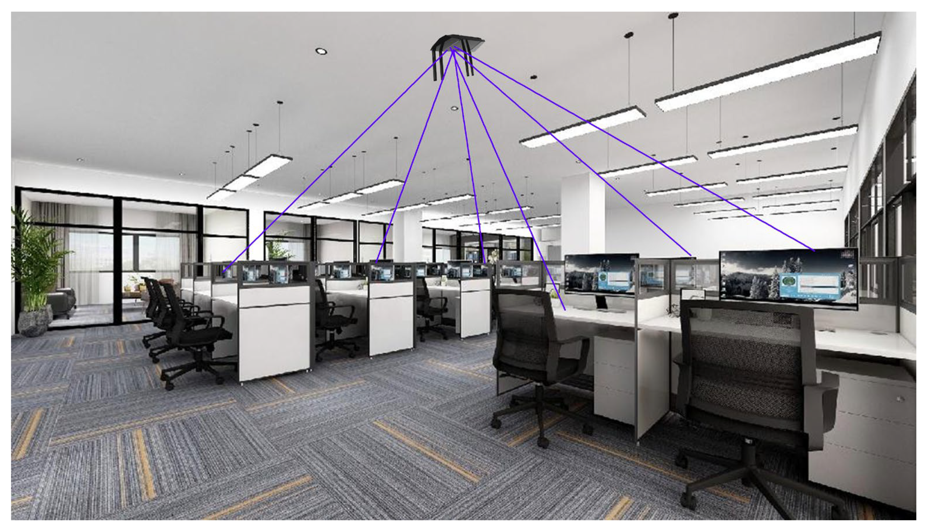
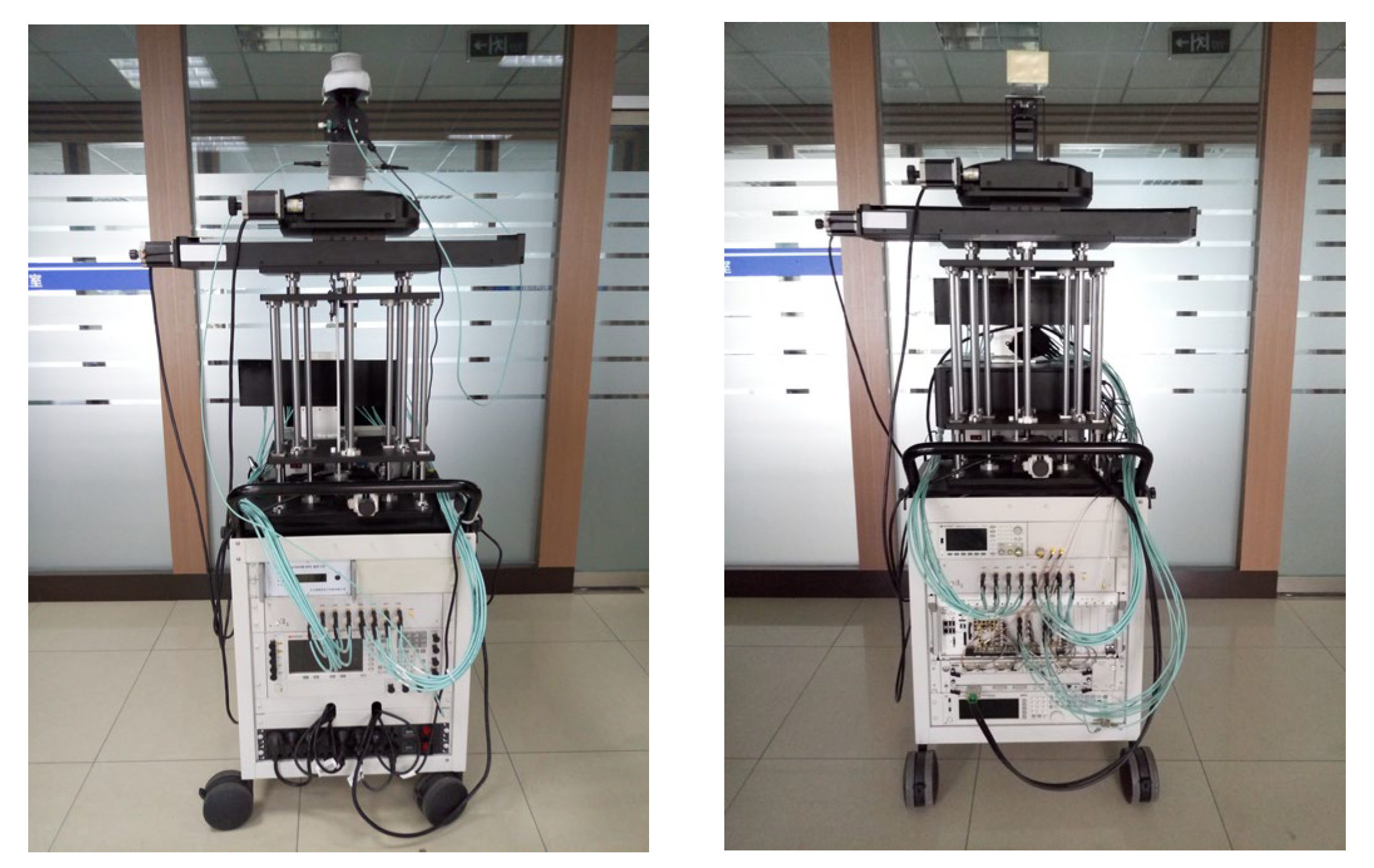
3. Channel Measurement in a Typical Open Indoor Environment

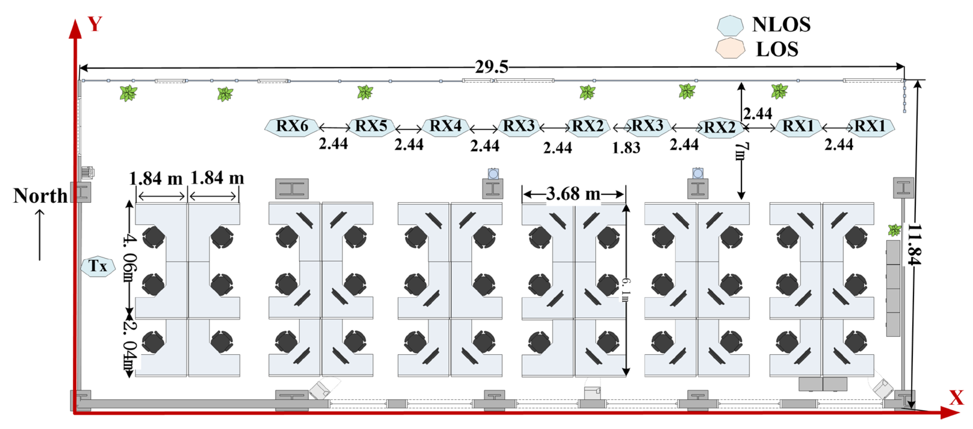
3.1. Channel Measurements in Office Scenarios

The channel measurement is performed in an office, as shown in Figure 4. The solid red lines represent the X- and Y-axes, and the direction of the building height is along the Z-axis. Moreover, light gray indicates the table, black is the stool and dark gray is the lime wall, and the greens are vegetation. An omnidirectional antenna that operates at 26.5~40 GHz is used at the transmitter (Tx); the transmitting antenna is located at (1.83, 5.35, 1.8), and the transmitting antenna is kept in a vertical polarization in the measurement. Moreover, a standard gain horn antenna of 26.3~40 GHz is used at the receiver (Rx), and the receiving antenna is vertically polarized and located in the aisle during the measurement. In this section, measurements are made at 28 GHz and 38 GHz. The radiation pattern of the transmitting antenna at 28 GHz is shown in Figure 5. In addition, both the E- and H-plane half-power beam widths are approximately 9° at 28 GHz. The radiation pattern of the receiving antenna at 38 GHz is shown in Figure 6. In addition, both the E- and H-plane half-power beam widths are approximately 7° at 38 GHz. It shows the higher the frequency is, the narrower the half-power beam width of the horn antenna is. Since there are five reinforced concrete load-bearing walls in the office, the measurement routes of the receiving points can be divided into line-of-sight (LOS) and non-line-of-sight (NLOS) arrays at 28 GHz and 38 GHz. As shown in Figure 4, there are six measuring points in LOS and three measuring points in NLOS at 28 GHz and 38 GHz.

Moreover, the position coordinates of the measurement points are (8.7, 9.7, 1.8), (11.14, 9.7, 1.8), (13.58, 9.7, 1.8), (16.02, 9.7, 1.8), (18.46, 9.7, 1.8), (20.29, 9.7, 1.8), (22.73, 9.7, 1.8), (25.17, 9.7, 1.8), (27.61, 9.7, 1.8) from west to east. The receiving antenna of each measurement point is rotated clockwise horizontally with an angular interval of 5° to form a virtual antenna array at 28 GHz and 38 GHz in the measurement. In addition, the MIMO channel detector test system used in this paper is shown in Figure 7; the measurement parameters are shown in

Table 1. The measurement parameters at 38 GHz and 28 GHz.

Physical Parameters	Value
Frequency(GHz)	28/38
Bandwidth (MHz)	500
Code length	1024
Transmitting antenna	Omnidirectional Antenna
Receiving antenna	Horn Antenna
Gain of transmitting antenna (dB)	4.5 (28 GHz); 6.2 (38 GHz)
Gain of receiving antenna (dB)	24.8 (28 GHz); 26.9 (38 GHz)
The height of receiver/transmitter antenna (m)	1.8/1.8
Transmission power (dBm)	0

.

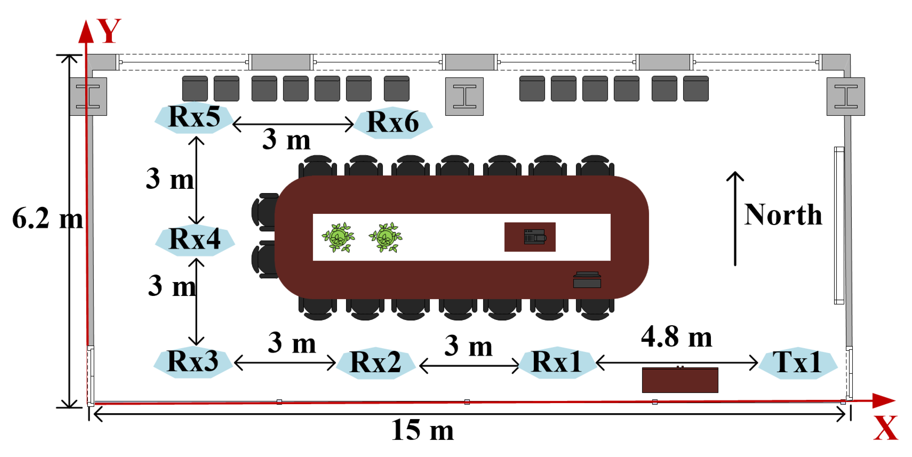
3.2. Channel Measurements in Conference Room Scenarios

The channel measurement in the conference room is described in this section. Channel measurements were carried out in a conference room at 39 GHz and 65.5 GHz, respectively.

At 39 GHz, an omnidirectional antenna is used in the transmitter, and a horn antenna is used in the receiver, and they are both vertically polarized. The radiation pattern of the receiving antenna at 39 GHz is shown in Figure 8. Moreover, both the E- and H-plane half-power beam widths are approximately 7°. Red indicates the table, black is the chair and light gray is the load-bearing wall in Figure 9. The transmitting antenna was fixed at the point (13.04, 1.16, 1.68); the receiving antenna was moved, and the positions of the receiving antenna from east to west were (8.24, 1.16, 1.68), (5.24, 1.16, 1.68), (2.24, 1.16, 1.68), (2.24, 2.96, 1.68), (2.24, 4.76, 1.68) and (5.24, 4.76, 1.68) in the measurement Moreover, the elevation angle of the horn antenna is set to −10°, −5°, 0° and 5° at each receiving position; the receiver is rotated horizontally at 5° intervals for each elevation angle to form a virtual antenna array. The parameters at 39 GHz are shown in

Table 2. The measurement parameters at 39 GHz.

Physical Parameters	Value
Frequency(GHz)	39
Bandwidth (GHz)	1
Code length	1024
Transmitting antenna	Omnidirectional Antenna
Receiving antenna	Horn Antenna
Gain of transmitting antenna (dB)	6.2
Gain of receiving antenna (dB)	26.92
The height of receiver/transmitter antenna (m)	1.68/1.68

.

At 65.5 GHz, the horn antennas are used at both the transmitter and the receiver. The operating frequency of the horn antennas is from 49.8 to 75.8 GHz with a standard gain of 20 dBi, and they are vertically polarized antennas. The radiation pattern of the horn antenna at 65.5 GHz is shown in Figure 10. In addition, the half-power beam widths in the E-plane and H-plane are approximately 13.94° and 13.83°, respectively. The transmitting antenna is fixed at (13.04, 1.16, 1.8), and the positions of the receiving antenna from east to west are (8.24, 1.16, 1.8), (5.24, 1.16, 1.8), (2.24, 1.16, 1.8), (2.24, 2.96, 1.8), (2.24, 4.76, 1.8) and (5.24, 4.76, 1.8) in the measurement. A horn antenna at the receiving end is adopted to move in the horizontal direction using a rotary table so that a virtual antenna array is formed. Moreover, it is moved eight times in the horizontal direction, and the horizontal distance is λ/2 each time. Since beamforming technology will be used in the millimeter wave and the transceiver antenna will use the direction of maximum gain to transmit and receive signals, the receiving antenna will always face the transmitting antenna at any point in the measurement. The test parameters at 65.5 GHz are shown in

Table 3. The measurement parameters at 65.5 GHz.

Physical Parameters	Value
Frequency(GHz)	65.5
Bandwidth (GHz)	1
Code length	1024
Transmitting antenna	Horn Antenna
Receiving antenna	Horn Antenna
Gain of transmitting antenna (dB)	21.68
Gain of receiving antenna (dB)	21.68
The height of receiver/transmitter antenna (m)	1.8/1.8

.

4. Analysis: Comparison of Theory and Experiments

4.1. Analysis in Office Scenarios

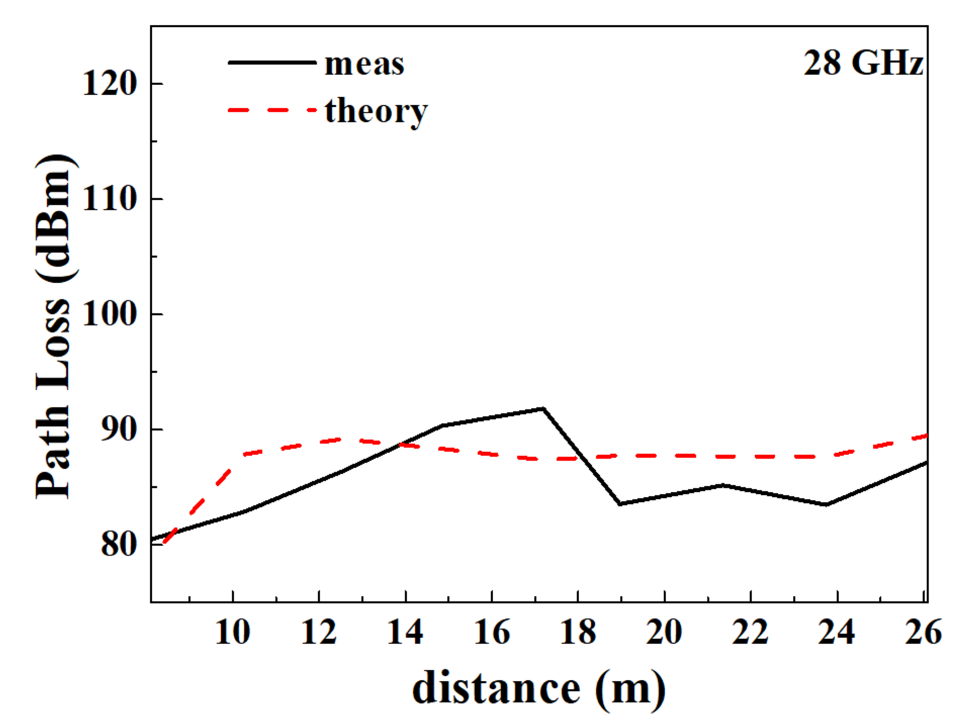
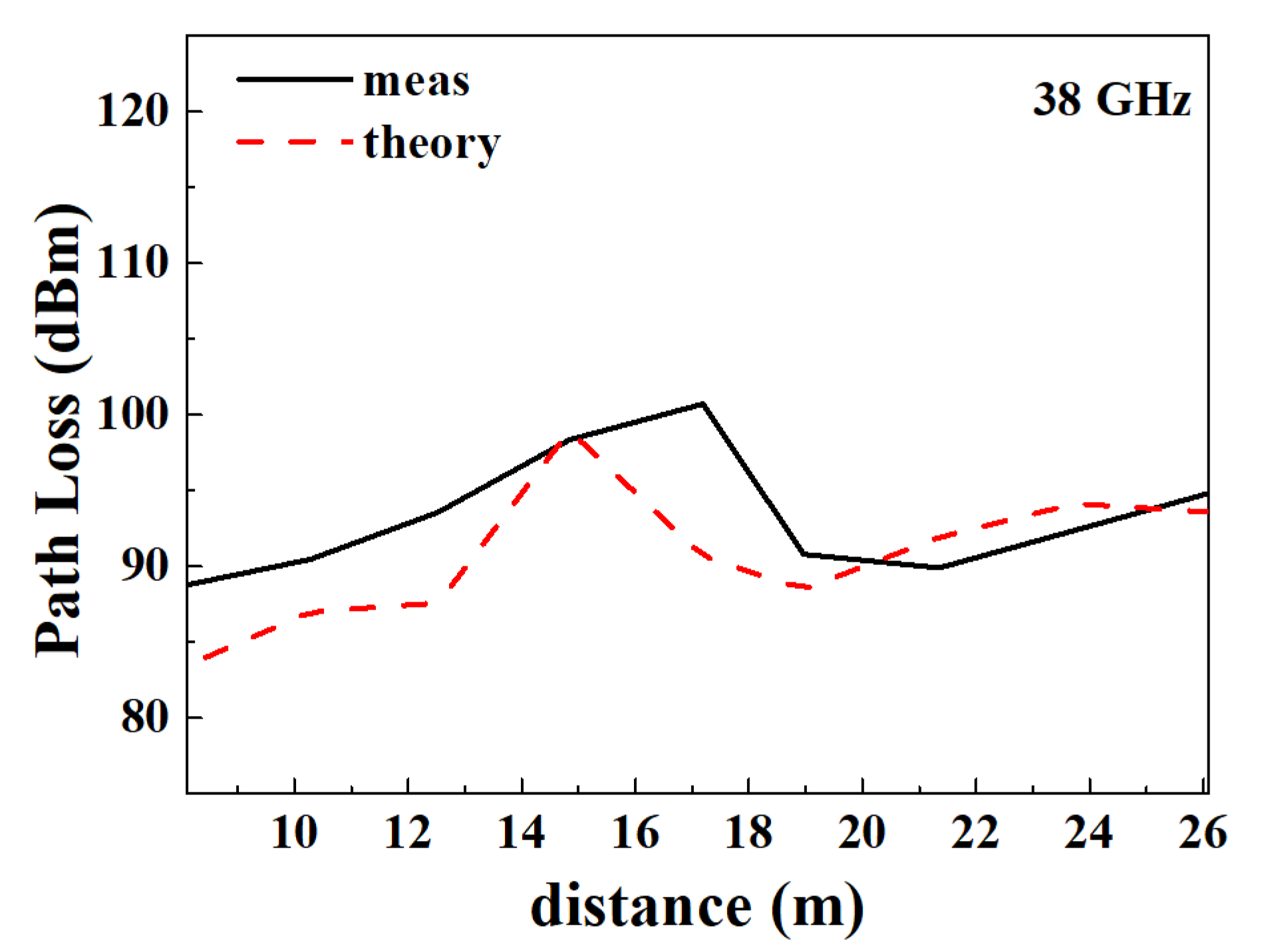
4.1.1. Analysis of Path Loss for 28 GHz and 38 GHz

The theoretical calculations consider the direct path, single reflection path, double reflection path and transmission from the transmitting antenna to the receiving antenna in this section. The X-axis indicates the distance between the transmitting and receiving antennas, the Y-axis is the path loss, ‘meas’ indicates the measured data which are represented by the black line and the blue line represents the theoretical calculations obtained using the ray tracing method in Figure 11 and Figure 12. As can be seen from the figures, in theory, the path loss increases overall with distance. The root-mean-square error (RMSE) between the theoretical calculation and the measured data is 3.418, and the mean absolute error (MAE) is 3.206 at 28 GHz, which reflects that the error between the predicted value and the experimental data at 28 GHz is very small in

Table 4. Comparison of RMSE and MAE at 28 GHz and 38 GHz.

Frequency/GHz	RMSE/dB	MAE/dB
28	3.418	3.206
38	4.6163	3.6485

. The RMSE between the theoretical calculation and the measured data at 38 GHz is 4.6163, and the MAE is 3.6485, which reflects that the error between the predicted value and the experimental data at 38 GHz, is also small. Therefore, the predicted value and the experimental data are in good agreement. The path loss at 38 GHz is greater than the path loss at 28 GHz, indicating that the higher the frequency is, the smaller the received electric field and the greater the path loss in Figure 11 and Figure 12.

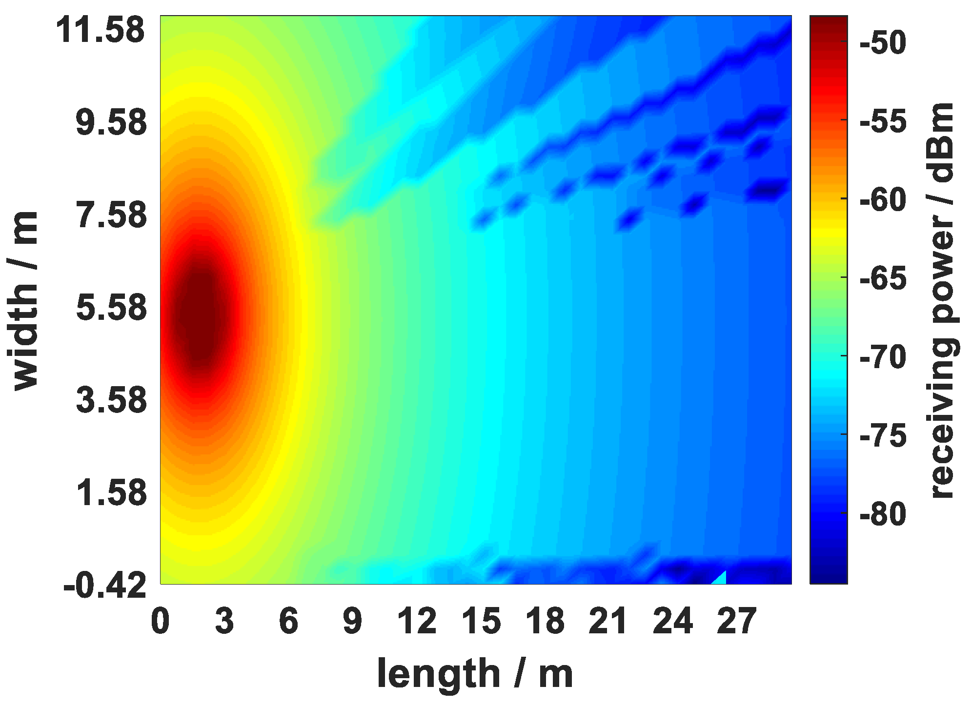
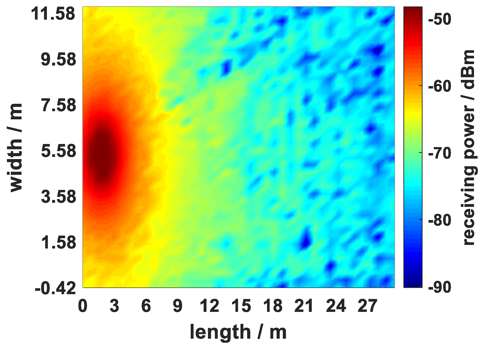
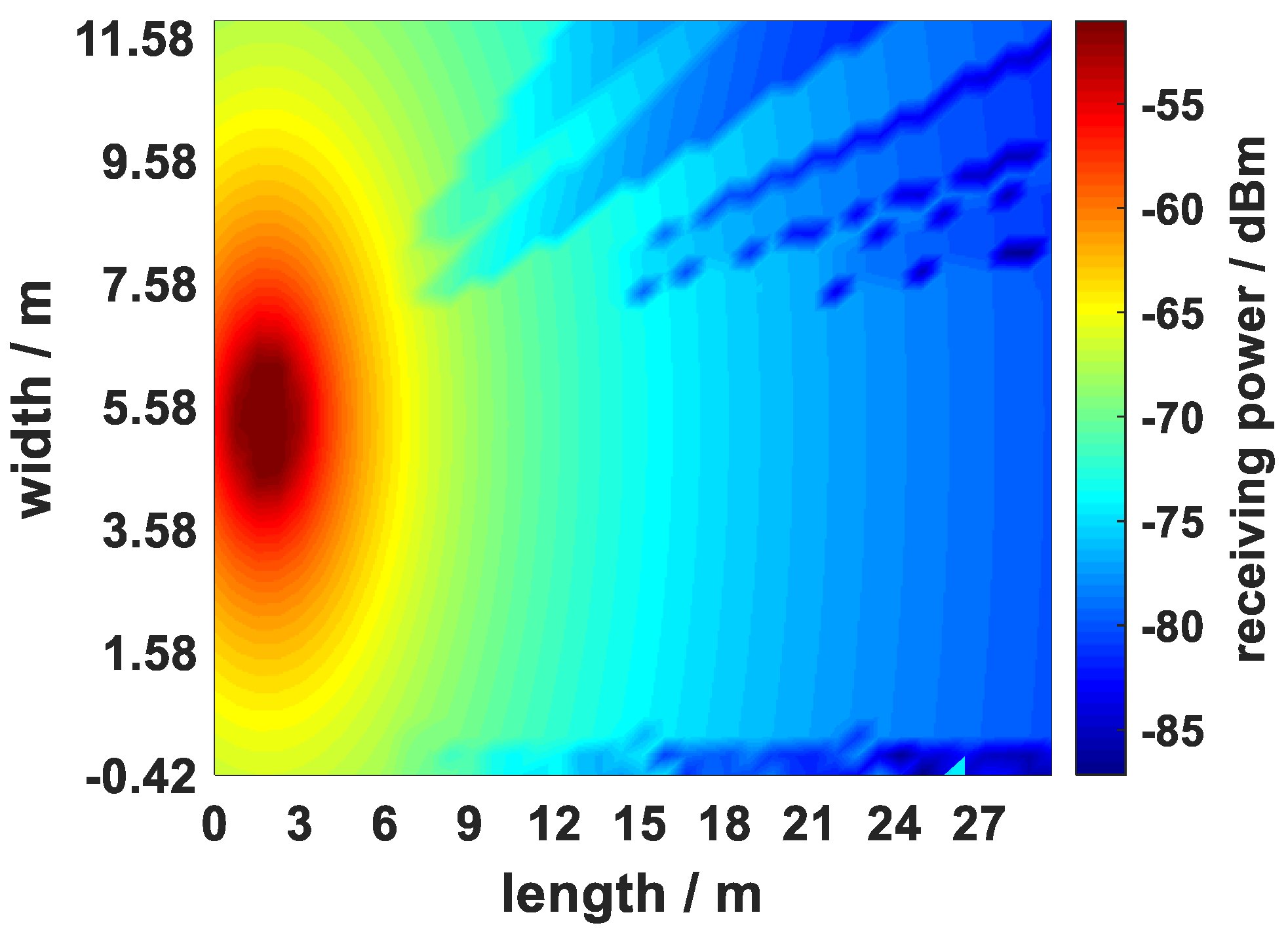
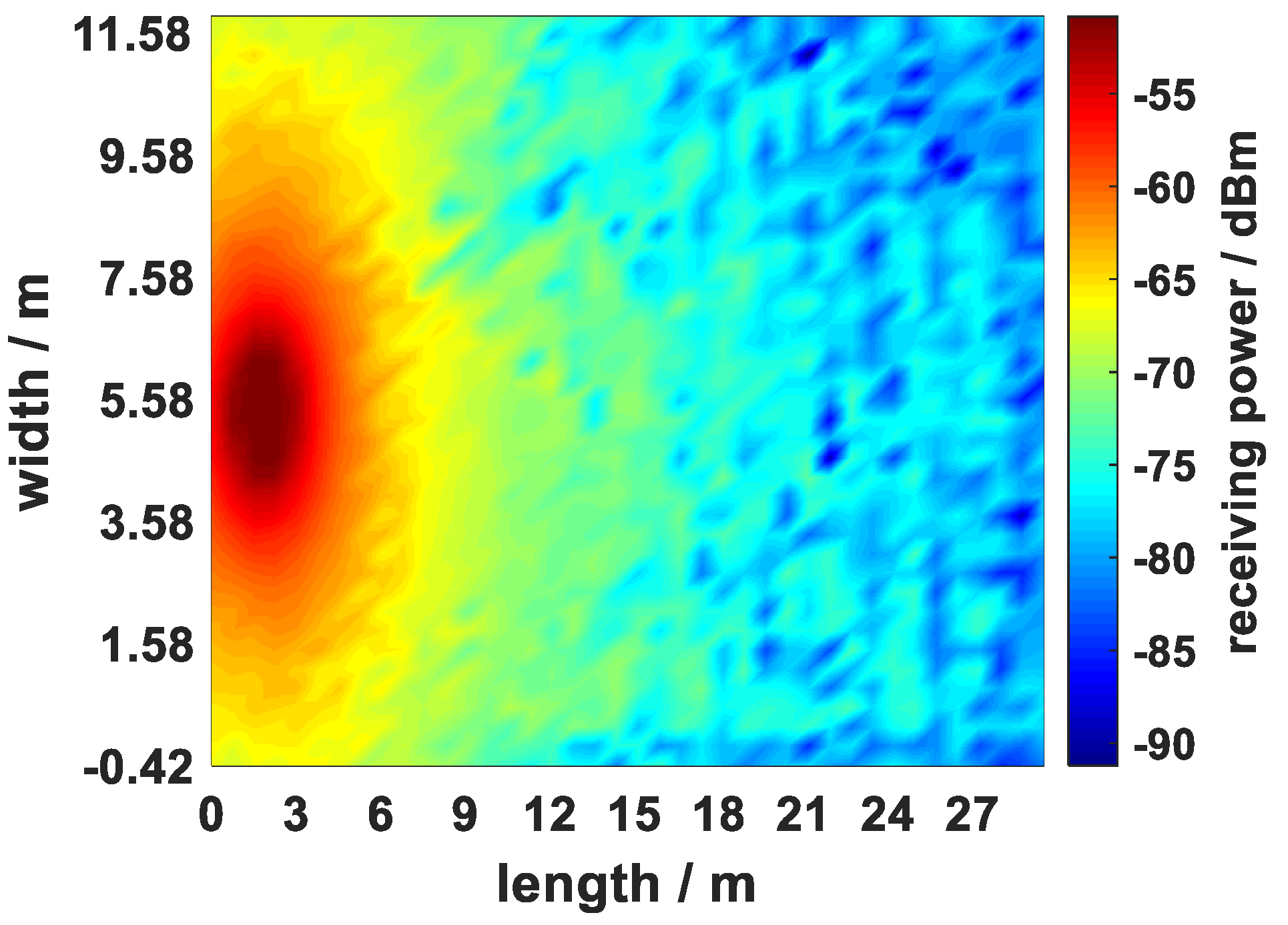
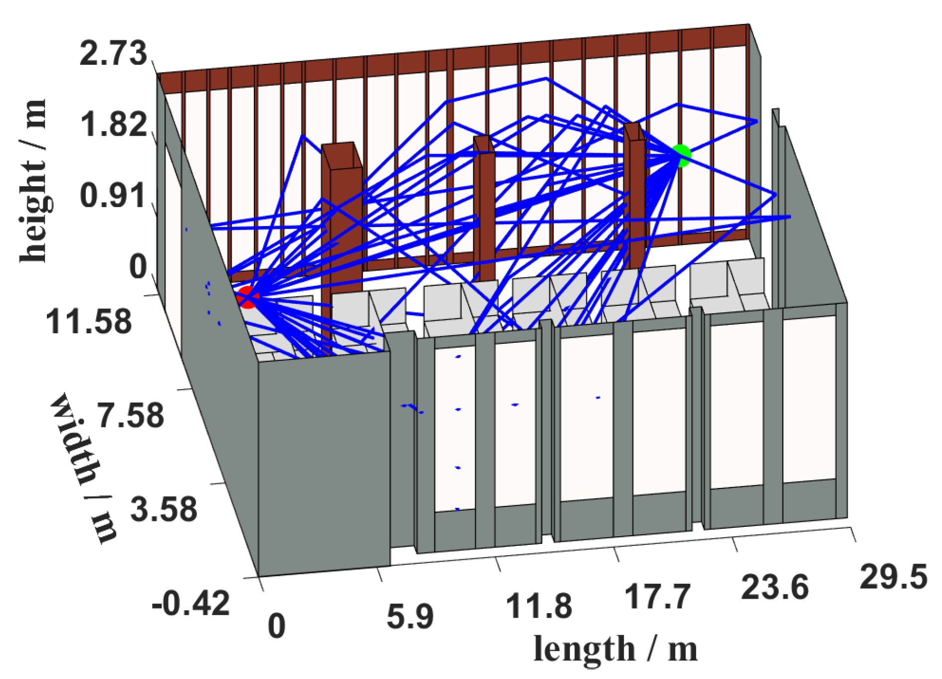
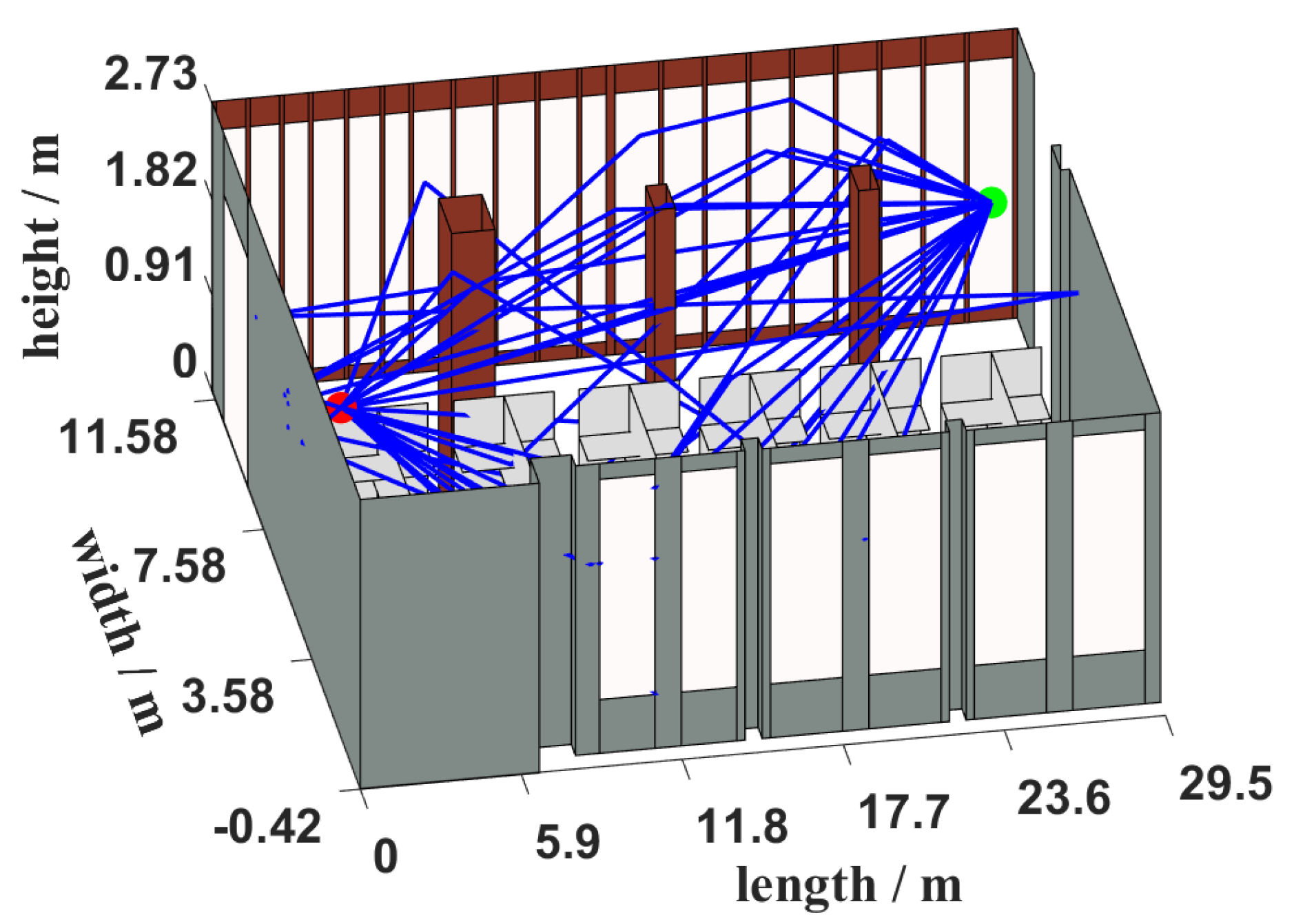
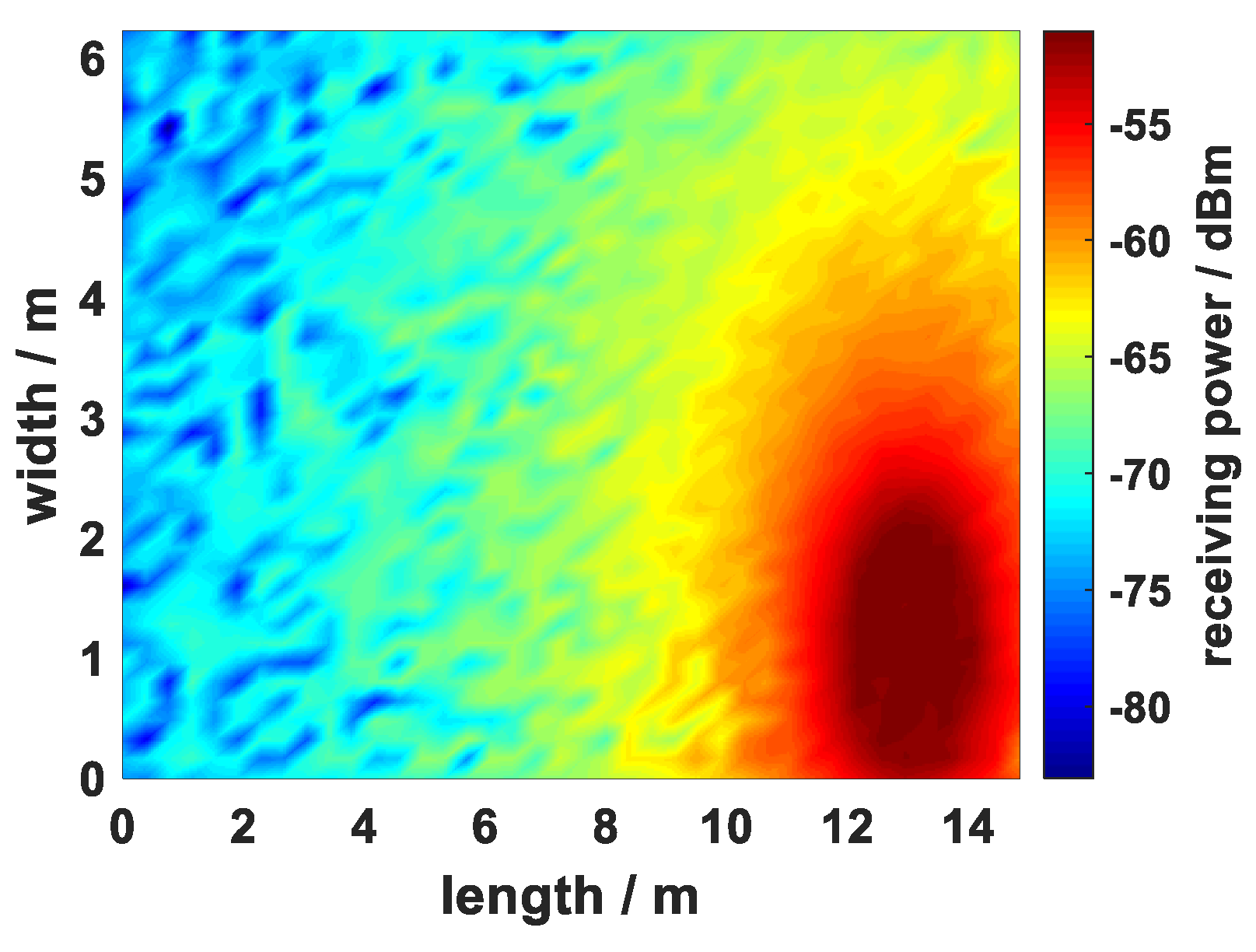
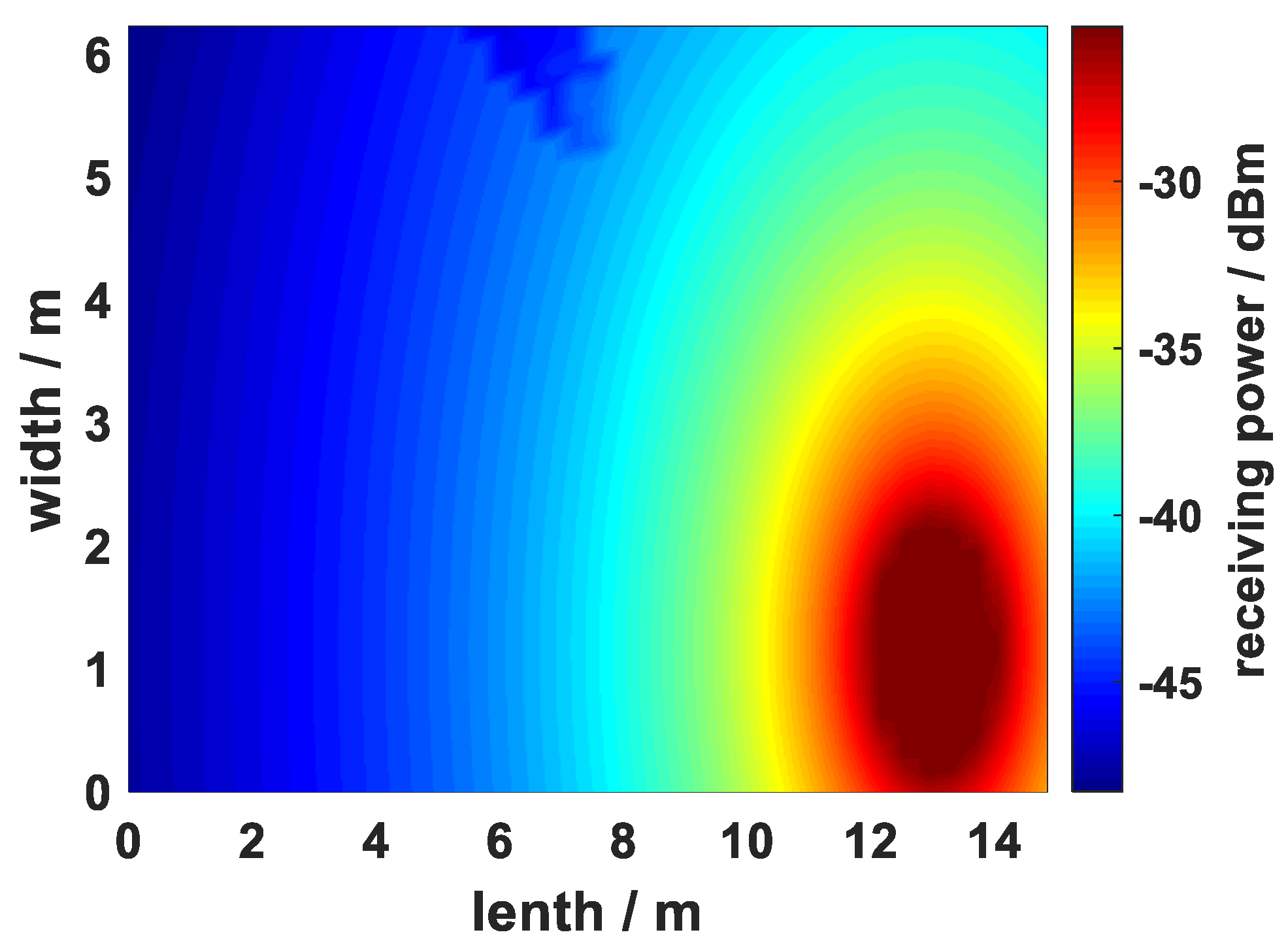
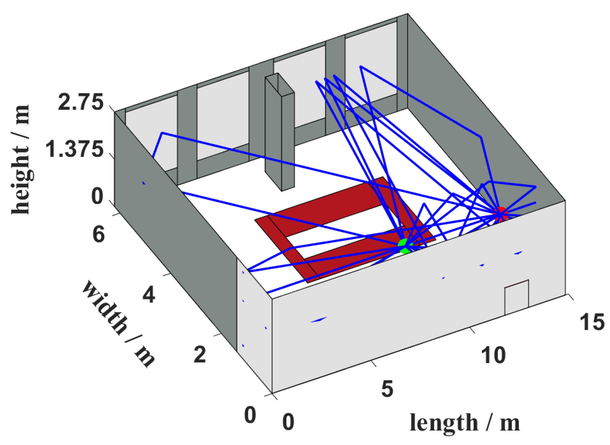
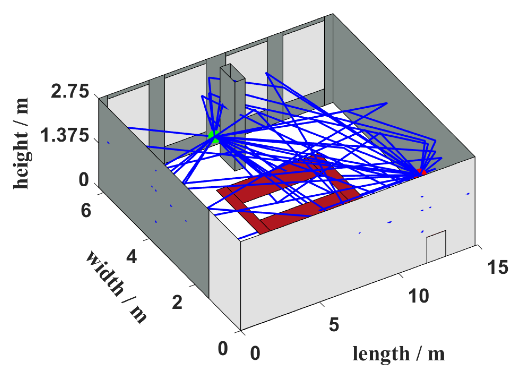
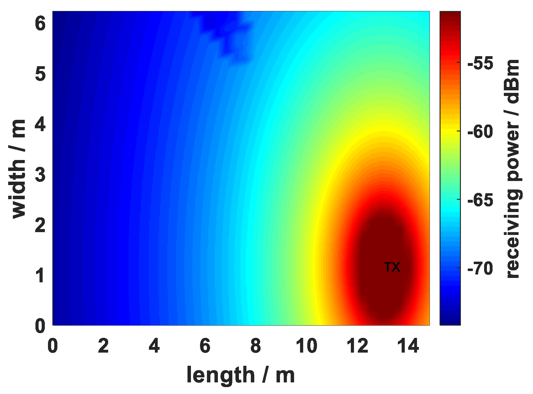
4.1.2. Analysis of Received Power and Ray Path Diagram for 28 GHz and 38 GHz

The received power of direct rays at 28 GHz is given when the transmit power is 0 dBm and the height of the receiving antenna is 1.8 m in Figure 13. It can be seen that there are three load-bearing walls respectively between 6 m and 9 m, between 12 m and 15 m, between 21 m and 24 m in length and between 6 m and 8 m in width. Moreover, the received power behind the load-bearing wall, which is close to the wall, decrease rapidly. It can be deduced that the transmitting antenna is located in the center of the reddest area, roughly between 0 m and 3 m in length and between 4 m and 6 m in width. The electric field around the transmitting antenna is the strongest, the received power around the transmitting antenna is the largest and the received power decreases gradually as the length and width increase or decrease, respectively.

The total received power between the transmitting antenna and each receiving antenna at 28 GHz is shown when the transmission power is 0 dBm and the height of the receiving antenna is 1.8 m in Figure 14. The maximum power is around the transmitting antenna. When the transmitting antenna is used as the center of the circle and the length is kept constant, the total received power decreases as the width increases or decreases. When the transmitting antenna is used as the center of the circle and the width is constant and the length is less than 12 m, the total received power decreases with increasing or decreasing length; when the length is greater than 12 m, the change is not obvious, which may be caused by the single reflection, double reflection and transmission between the ray and the lime wall, glass wall or table. However, the total received power does not change much.

The received power of the direct rays at 38 GHz is shown in Figure 15 when the transmit power is 0 dBm and the height of the receiving antenna is 1.8 m. It can be seen that the received power of the direct ray at 38 GHz in Figure 15 appears to be the same as the received power of the direct ray at 28 GHz in Figure 13. The overall color of the received power graph at 38 GHz in Figure 15 is lighter than the overall color of the received power graph at 28 GHz in Figure 13. This shows that the received power at each position at 38 GHz in Figure 15 is less than the received power at each position corresponding to 28 GHz in Figure 13, by approximately 5 dBm, indicating that the higher the frequency is, the less the received power is.

Figure 16 shows the total received power between the transmitting antenna and receiving antenna at 38 GHz. The total received power graph at 38 GHz in Figure 16 appears the same as the total received power graph at 28 GHz in Figure 14, and the total received power at 38 GHz in Figure 16 is less than the total received power at 28 GHz in Figure 14. This shows that the higher the frequency is, the less the received power under the same conditions. The comparison of the received power at different frequencies is of great significance in frequency selection.

The multipaths of the receiving points using ray tracing at 28 GHz are shown in LOS and NLOS, respectively, as illustrated in Figure 17 and Figure 18. The red dot indicates the transmitting point, the green dot is the receiving point and the blue line is the ray path in Figure 17 and Figure 18. There are many rays from the transmitting antenna to the receiving antenna. Moreover the number of rays from the transmitting point to different receiving point is different, and the ray path is also different in Figure 17 and Figure 18. Since the positions of the transmitting and receiving antennas at 28 GHz are the same as the positions of the transmitting and receiving points at 38 GHz during the measurements, the three-dimensional ray path diagrams in LOS and NLOS at 38 GHz are the same as those at 28 GHz. However, the electric field intensity of each ray is different.

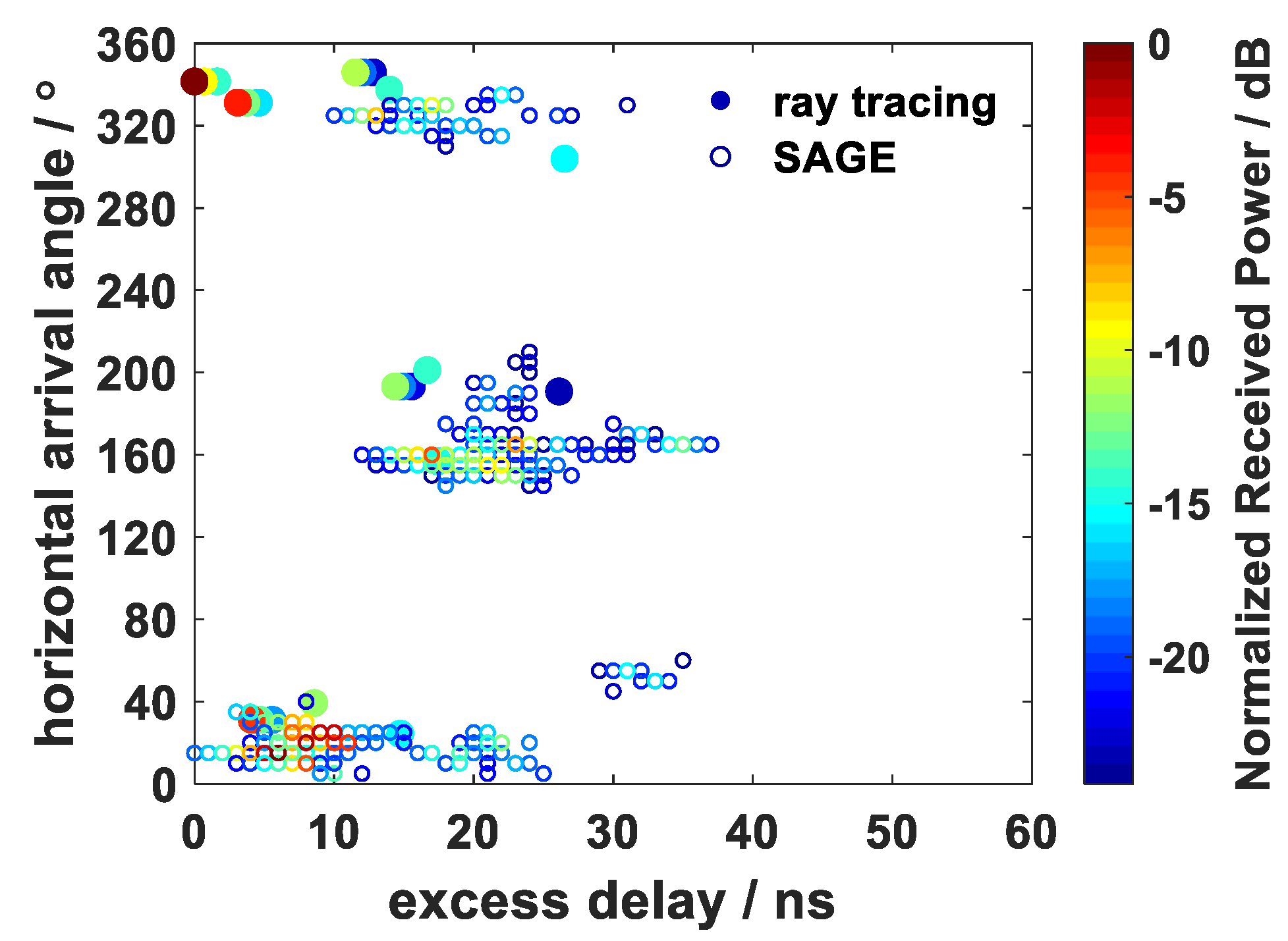
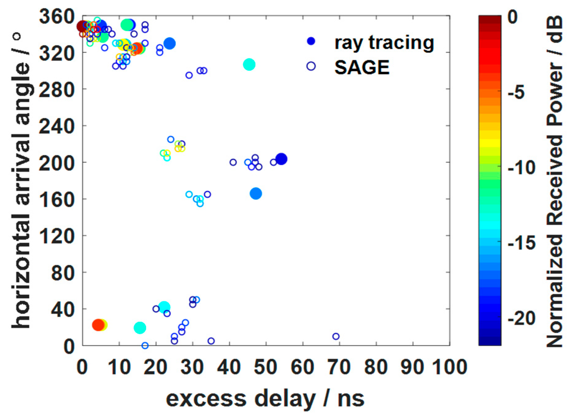
4.1.3. Analysis of SAGE Algorithm for 28 GHz and 38 GHz

The following multipath parameters are extracted in the measured channel impulse response using the SAGE algorithm: time delay, amplitude and horizontal arrival angle of each ray path in the section. When running the SAGE algorithm, the multipath number is set to 200, the iteration number is set to 50 and the multipath power threshold is set to −22 dB. Information that is useful for the multipath analysis can be filtered from 200 ray paths. The comparison between the multipath obtained by the SAGE algorithm and the multipath calculated by the ray tracing method is shown in Figure 19 and Figure 20. The solid circles indicate the multipath calculated by the three-dimensional ray tracing method, and the hollow circles are the multipath obtained by processing the measured data using the SAGE algorithm. The abscissa denotes the excess delay, and the vertical coordinate is the horizontal arrival angle.

The multipath information of the second measurement point (22.73, 9.7, 1.8) in LOS at 28 GHz is analyzed in Figure 19. The multipath information of the first reception point (25.17, 9.7, 1.8) in LOS at 38 GHz is analyzed in Figure 20. When the horizontal arrival angle is in the vicinity of 330° and the excess delay is 0 ns, the signal is the strongest in Figure 19 and Figure 20. This indicates that the signal transmitted by the transmitting antenna reaches the receiving antenna directly at this time. The receiving antenna is a horn antenna, and the half-power beam width in the E- and H-planes is approximately 7°. The signals are collected at 5° intervals by the receiving antenna so that a virtual antenna array can be formed. Therefore, the signal can be received at a horizontal arrival angle of between 140° and 240° in Figure 19 and Figure 20. When the receiving antenna was rotated to roughly between 280° and 360° and between 0° and 60°, there are two clusters, both of which are visible in Figure 19 and Figure 20. This could be due to the reflections caused by the roof, the wall around the desk and the glass. Since the material of the measurement environment is glass and lime walls in the office, the multipath signals are mainly extracted from specular reflections. Compared to the ray tracing method, richer multipath information is obtained using the SAGE algorithm in Figure 19 and Figure 20. This may be caused by scattering from the lime wall. The overlap of the three clusters obtained using the ray tracing method and the sage algorithm, respectively, indicates that the proposed ray tracing method is applicable to indoor environments.

However, the number of multipaths obtained using the SAGE algorithm in Figure 19 is more than the number of multipaths in Figure 20.

4.2. Analysis in Conference Room Scenarios

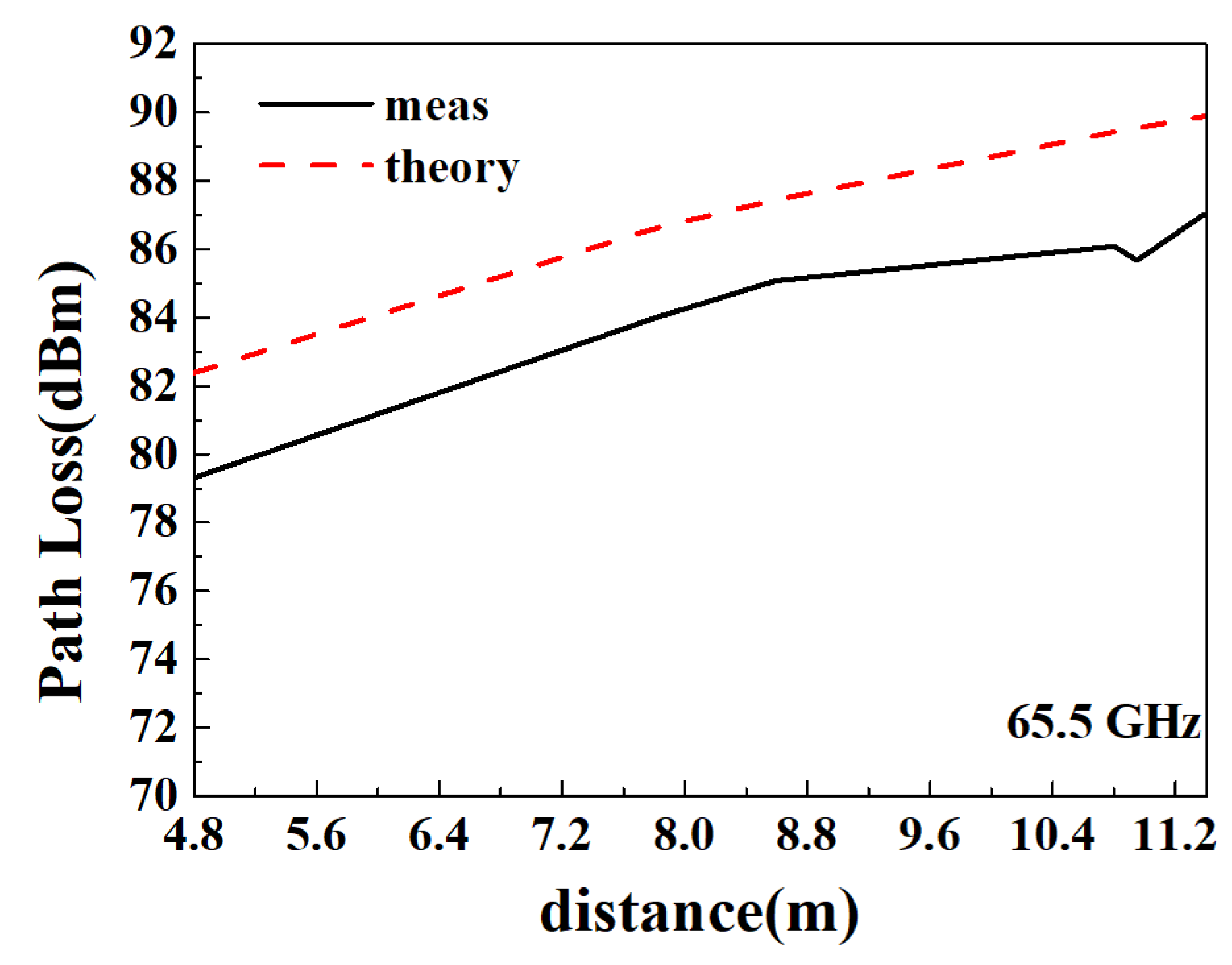
4.2.1. Analysis of Path Loss for 39 GHz and 65.5 GHz

The channel characterization is analyzed for the conference room scenario in this section. The X-axis is the distance between the transmitting and receiving antennas and the Y-axis is the path loss in Figure 21 and Figure 22. When the transmitting and receiving antennas are in a straight line, that is, the receiving points are located at Rx1, Rx2 and Rx3 the path loss increases with the distance in Figure 21. As shown in

Table 5. Comparison of RMSE and MAE at 39 GHz and 65.5 GHz.

Frequency/GHz	RMSE/dB	MAE/dB
39	2.1722	1.7233
65.5	3.0669	3.0276

, the RMSE between the theoretical calculation obtained using the ray tracing method and the test data at 39 GHz is 2.1722, and the MSE is 1.7233, indicating that the theoretical calculation obtained using the ray tracing method and the test data are in good agreement.

The path loss increases with the distance between the transmitting and receiving antennas in Figure 22. The RMSE between the theoretical calculations obtained by using the ray tracing method and test data is 3.1016, and the MSE is 3.0683 at 65.5 GHz in Table 5. Therefore, the theoretical calculations obtained by using the ray tracing method agree well with the test data, which indicates that the ray tracing method is suitable for indoor scenes at 65.5 GHz. Overall, at each measurement location, the path loss at 39 GHz in Figure 21 is less than the path loss at 65.5 GHz in Figure 22. The theoretically calculated path loss at 65.5 GHz in Figure 22 reaches approximately 90 dBm, and the theoretically calculated path loss at 39 GHz in Figure 21 reaches approximately 85 dBm. This means that the difference between the path loss at 65.5 GHz and the path loss at 39 GHz is approximately 5 dBm.

4.2.2. Analysis of Received Power and Ray Path Diagram for 39 GHz and 65.5 GHz

The received power distribution is given in this section. Only the direct rays between the transmitting antenna and the receiving antenna are calculated in Figure 23. The point with the reddest color is the transmitting antenna. Moreover, the further the measurement point is away from the transmitting point, the less the received power is. Since there is a load-bearing wall between 8 m and 10 m in length and 5 m and 6 m in width, the received power decreases rapidly after passing through the load-bearing wall.

The total received power is calculated in Figure 24. The reddest position indicates the location of the transmitting antenna and the location of the load-bearing wall cannot be seen. Moreover, calculations of single reflection, double reflection and transmission make the received power decrease slowly, and the received power is more accurate. When the length is from 4 m to 11 m and the width is from 1.5 m to 4 m, the received power is probably between −70 and −65 dBm, which is much less than the received power around the transmitting point. Therefore, it is not recommended to place the base station in the corner.

The diagram of the received power is shown at 65.5 GHz in this section. The power distribution of the direct rays from the transmitting antenna to the receiving antenna is shown when the transmission power is 0 dBm and the height of the receiving antenna is 1.8 m in Figure 25. A horn antenna is adopted in the transmitter. However, the antenna aperture of the transmitting antenna is always facing that of the receiving antenna. Moreover, as the measurement point moves further away from the transmitting antenna, the received power gradually decreases, as shown in Figure 25. An omnidirectional antenna is used in the transmitter, and the gain is 6.2 dB at 39 GHz; a standard gain horn antenna is adopted in the receiver, and the gain is 26.92 dB at 39 GHz; standard gain horn antennas are used at the transmitter and receiver, and the gain is 21.68 dB at 65.5 GHz. Since the total gain of the antennas at 65.5 GHz is higher than that of the antennas at 39 GHz, the received power at 65.5 GHz is greater than that at 39 GHz. There is a load-bearing wall between 8 m and 10 m in length and between 5 m and 6 m in width, and the received power decreases rapidly after passing through the load-bearing wall.

Figure 26 shows the distribution of the total receiving power at each receiving point when the transmit power is 0 dBm and the height of the receiving antenna is 1.8 m. The phenomenon in Figure 26 is the same as that in Figure 25, indicating that the single and double reflections between the transmitting and receiving antennas are very small and almost negligible. This shows that the use of beamforming in the millimeter wave can greatly improve the received power at each receiving end.

The diagram of the three-dimensional ray path between the transmitting and receiving antennas using ray tracing at 39 GHz is shown in Figure 27 and Figure 28. The light gray is the glass, the dark gray is the lime wall and the load-bearing wall and the red is the table. Moreover, the red dot is the transmitting antenna, the green dot is the receiving antenna and the blue line is the multipath between the transmitting and receiving antennas. As can be seen, there are rich multipaths between the transmitting and receiving antennas in Figure 27 and Figure 28. The number of rays is different and the ray paths are different when the receiving antenna is at different locations in Figure 27 and Figure 28. However, the locations of transmitting and receiving antennas at 65.5 GHz are the same as those at 39 GHz. Only the transmitting and receiving antennas used at 65.5 GHz are different from those used at 39 GHz. Therefore, the diagrams of the three-dimensional ray paths at 65.5 GHz are exactly the same as those at 39 GHz, but the electric field intensity of each ray at 65.5 GHz is different from that at 39 GHz.

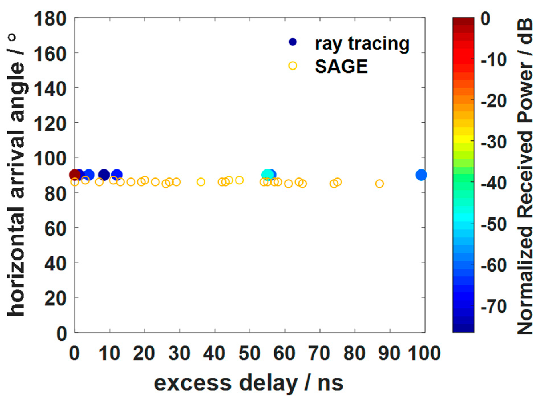
4.2.3. Analysis of the SAGE Algorithm for 39 GHz and 65.5 GHz

The SAGE algorithm is used to extract the time delay, horizontal arrival angle and amplitude of measured data. The initial values in the SAGE algorithm are set, that is, the number of iterations is 50, the maximum number of multipaths is 200 and the received power threshold is set to −25 dB so that the useful multipath is filtered from the 200 multipaths in Figure 29. It can be seen that the reddest point is located with an excess delay of 0 ns and a horizontal arrival angle between 320° and 360° when the ray tracing method is adopted in Figure 29. In addition, the multipaths obtained by the SAGE algorithm are richer compared to those obtained by using ray tracing, which may be due to the scattering effect. Moreover, there is a total of three clusters in Figure 29. When the horizontal arrival angle is between 140° and 220°, the first cluster may be caused by the reflection of the lime wall, which is directly opposite the transmitting antenna; the second cluster with a horizontal arrival angle between 0° and 60° may be caused by the reflection of the wall, glass and roof on the right; and the third cluster with a horizontal arrival angle between 300° and 360° may be caused by the reflection of the glass wall and roof. The number of clusters obtained using the ray tracing method overlaps with the number of clusters obtained using the SAGE algorithm. It shows that the proposed ray tracing method can simulate the real scenario very well.

The comparison of using the SAGE algorithm and ray tracing method at 65.5 GHz at the first reception point (8.24, 1.16, 1.68) is shown in Figure 30. Since the transmitting and receiving antennas are always facing each other, all the rays occur with a horizontal arrival.

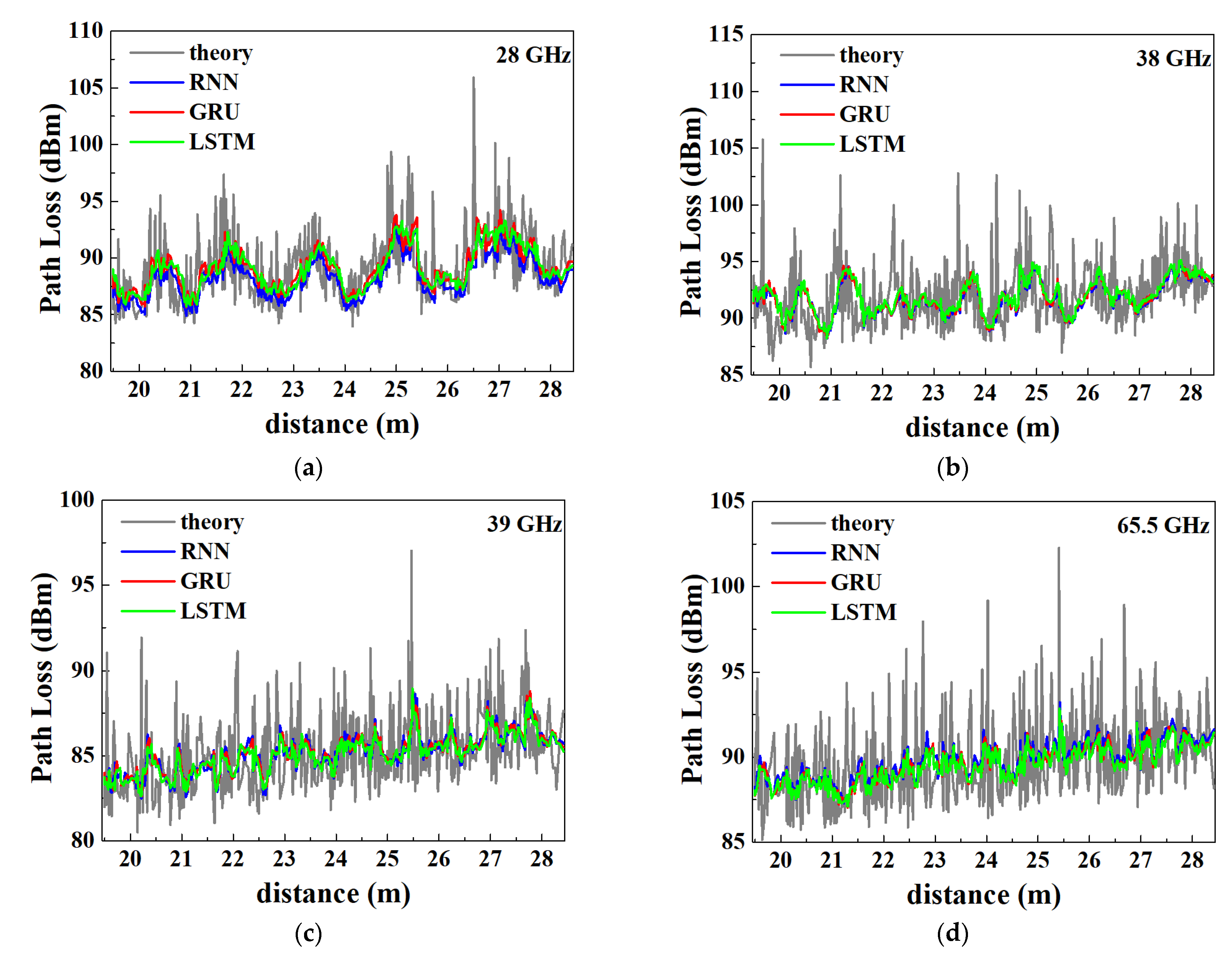
4.3. Predicting the Path Loss Using Deep Learning Models

In this paper, the path loss of 1600 receiving points is calculated using the ray tracing method when the transmitting point is fixed. The front 70% of the path losses is used for training sets, and the remaining 30% is used for test sets. This paper verifies the performance of the RNN, GRU and LSTM networks in sequence prediction based on four sets of propagation loss data at 28 GHz, 38 GHz, 39 GHz and 65.5 GHz. The path losses predicted by the RNN, GRU and LSTM networks do not differ much but differ greatly from the original sequence in Figure 31. The abscissa ‘distance’ indicates the distance of the receiving antenna from the transmitting antenna. As shown in

Table 6. Comparison of RMSE and MAE at different frequency bands.

Frequency (GHz)	28	38	39	65.5
ERROR	RMSE/MAE (dB)	RMSE/MAE (dB)	RMSE/MAE (dB)	RMSE/MAE (dB)
RNN	2.635/1.8813	2.7284/2.7284	2.2648/1.7827	2.4447/1.9061
GRU	2.5046/1.8628	2.7055/1.9773	2.2342/1.7593	2.4152/1.8362
LSTM	2.4949/1.8451	2.6881/1.9745	2.2091/1.7328	2.4041/1.8164

, the RMSEs of the RNN, GRU and LSTM networks do not vary much, and their MAEs also do not vary much in the same frequency band. Compared with other methods, the RMSE and MAE of the LSTM method are the smallest, and the LSTM method has a better fit for the sequence of propagation loss predicted at a longer distant, which can better reflect the propagation trend and value of electromagnetic waves.

5. Conclusions

In this paper, a fast and accurate method is studied to obtain the path loss of all points indoors in the millimeter wave band by the following three aspects. First, a three-dimensional ray tracing method suitable for indoor scenes is presented based on geometric optics theory, the uniform theory of diffraction and image theory. Then, the channel measurements were carried out in different frequency bands for office and conference rooms, and the SAGE algorithm was used to process the measured data. Compared with the results obtained from the SAGE algorithm, it is verified whether the presented three-dimensional ray tracing method is applicable in indoor scenes; the wireless channel parameters of indoor scenes are analyzed. Finally, three deep learning models (RNN, GRU, LSTM) are used to predict the path loss at different distances. The study shows that the received electric field is smaller and the path loss is larger when the frequency is higher. Since both RMSE and MAE between the theoretical calculation and the measured data are small at different frequency bands and the number of clusters obtained by the ray tracing method overlaps with the number of clusters obtained by the SAGE algorithm, the three-dimensional ray tracing method considering line of sight, reflection or transmission is suitable for indoor environments. Moreover, the LSTM method is more suitable for the sequence of predicted path loss compared with the RNN and GRU methods. The authors will conduct further measurements and analyses in other conference rooms and office scenarios, which will provide more reliable statistics for the layout of base stations in a typical open indoor environment such as 5G millimeter wave conference rooms.

References

1. Mitra, R.N.; Agrawal, D.P. 5G mobile technology: A survey. ICT Express 2015, 1, 132–137. [Google Scholar] [CrossRef]
2. Hur, S.; Baek, S.; Kim, B.; Chang, Y.; Molisch, A.F.; Rappaport, T.S.; Haneda, K.; Park, J. Proposal on millimeter-wave channel modeling for 5G cellular system. IEEE J. Sel. Top. Signal Process. 2016, 10, 454–469. [Google Scholar] [CrossRef]
3. del Peral-Rosado, J.; Granados, G.; Raulefs, R.; Leitinger, E.; Grebien, S.; Wilding, T.; Dardari, D.; Lohan, E.; Wymeersch, H.; Floch, J. Whitepaper on new localization methods for 5G wireless systems and the Internet-of-Things. In White Paper of the COST Action CA15104 (IRACON); COST Action CA15104, IRACON; 2018; pp. 1–27. Available online: https://re.public.polimi.it/bitstream/11311/1069386/2/2018_white_paper_IRACON-WP2.pdf (accessed on 30 May 2023).
4. Papazian, P.B.; Gentile, C.; Remley, K.A.; Senic, J.; Golmie, N. A radio channel sounder for mobile millimeter-wave communications: System implementation and measurement assessment. IEEE Trans. Microw. Theory Tech. 2016, 64, 2924–2932. [Google Scholar] [CrossRef]
5. Rappaport, T.S.; Xing, Y.; MacCartney, G.R.; Molisch, A.F.; Mellios, E.; Zhang, J. Overview of millimeter wave communications for fifth-generation (5G) wireless networks—With a focus on propagation models. IEEE Trans. Antennas Propag. 2017, 65, 6213–6230. [Google Scholar] [CrossRef]
6. Jondhale, S.R.; Mohan, V.; Sharma, B.B.; Lloret, J.; Athawale, S.V. Support vector regression for mobile target localization in indoor environments. Sensors 2022, 22, 358. [Google Scholar] [CrossRef]
7. Yun, Z.; Iskander, M.F. Ray tracing for radio propagation modeling: Principles and applications. IEEE Access 2015, 3, 1089–1100. [Google Scholar] [CrossRef]
8. Geok, T.K.; Hossain, F.; Kamaruddin, M.; Rahman, N.; Thiagarajah, S.; Chiat, A.T.W.; Liew, C. A comprehensive review of efficient ray-tracing techniques for wireless communication. Int. J. Commun. Antenna Propag. 2018, 8, 123–136. [Google Scholar] [CrossRef]
9. Cao, Y.-W.; Liu, Z.-Y.; Guo, L.-X. A Fast Ray-tracing-based Algorithm for Very Low Frequency Radio Propagation. In Proceedings of the 2019 Cross Strait Quad-Regional Radio Science and Wireless Technology Conference (CSQRWC), Taiyuan, China, 18–21 July 2019; IEEE: Piscataway, NJ, USA, 2019; pp. 1–2. [Google Scholar]
10. Rubio, L.; Peñarrocha, V.M.R.; Cabedo-Fabres, M.; Bernardo-Clemente, B.; Reig, J.; Fernández, H.; Pérez, J.R.; Torres, R.P.; Valle, L.; Fernández, Ó. Millimeter-Wave Channel Measurements and Path Loss Characterization in a Typical Indoor Office Environment. Electronics 2023, 12, 844. [Google Scholar] [CrossRef]
11. Lawton, M.; Davies, R.; McGeehan, J.P. A ray launching method for the prediction of indoor radio channel characteristics. In Proceedings of the IEEE International Symposium on Personal, Indoor and Mobile Radio Communications, Bristol, UK, 23–25 September 1991; IEEE: Piscataway, NJ, USA, 1991; pp. 104–108. [Google Scholar]
12. Fortune, S. Efficient algorithms for prediction of indoor radio propagation. In Proceedings of the VTC’98, 48th IEEE Vehicular Technology Conference, Pathway to Global Wireless Revolution (Cat. No. 98CH36151), Ottawa, ON, Canada, 21 May 1998; IEEE: Piscataway, NJ, USA, 1998; pp. 572–576. [Google Scholar]
13. Hoppe, R.; Wertz, P.; Landstorfer, F.M.; Wölfle, G. Advanced ray-optical wave propagation modelling for urban and indoor scenarios including wideband properties. Eur. Trans. Telecommun. 2003, 14, 61–69. [Google Scholar] [CrossRef]
14. Degli-Esposti, V.; Falciasecca, G.; Fuschini, F.; Vitucci, E. A meaningful indoor path-loss formula. IEEE Antennas Wirel. Propag. Lett. 2013, 12, 872–875. [Google Scholar] [CrossRef]
15. Wallace, J.W.; Ahmad, W.; Yang, Y.; Mehmood, R.; Jensen, M.A. A comparison of indoor MIMO measurements and ray-tracing at 24 and 2.55 GHz. IEEE Trans. Antennas Propag. 2017, 65, 6656–6668. [Google Scholar] [CrossRef]
16. Geok, T.K.; Hossain, F.; Chiat, A.T.W. A novel 3D ray launching technique for radio propagation prediction in indoor environments. PLoS ONE 2018, 13, e0201905. [Google Scholar] [CrossRef] [PubMed]
17. He, D.; Ai, B.; Guan, K.; Wang, L.; Zhong, Z.; Kürner, T. The design and applications of high-performance ray-tracing simulation platform for 5G and beyond wireless communications: A tutorial. IEEE Commun. Surv. Tutor. 2018, 21, 10–27. [Google Scholar] [CrossRef]
18. Chen, Y.-S.; Lai, F.-P.; You, J.-W. Analysis of antenna radiation characteristics using a hybrid ray tracing algorithm for indoor WiFi energy-harvesting rectennas. IEEE Access 2019, 7, 38833–38846. [Google Scholar] [CrossRef]
19. Hossain, F.; Geok, T.K.; Rahman, T.A.; Hindia, M.N.; Dimyati, K.; Ahmed, S.; Tso, C.P.; Abd Rahman, N.Z. An efficient 3-D ray tracing method: Prediction of indoor radio propagation at 28 GHz in 5G network. Electronics 2019, 8, 286. [Google Scholar] [CrossRef]
20. Obeidat, H.; Alabdullah, A.; Elkhazmi, E.; Suhaib, W.; Obeidat, O.; Alkhambashi, M.; Mosleh, M.; Ali, N.; Dama, Y.; Abidin, Z. Indoor environment propagation review. Comput. Sci. Rev. 2020, 37, 100272. [Google Scholar] [CrossRef]
21. Ullah, U.; Kamboh, U.R.; Hossain, F.; Danish, M. Outdoor-to-indoor and indoor-to-indoor propagation path loss modeling using smart 3D ray tracing algorithm at 28 GHz mmWave. Arab. J. Sci. Eng. 2020, 45, 10223–10232. [Google Scholar] [CrossRef]
22. Lee, J.-H.; Choi, J.-S.; Lee, J.-Y.; Kim, S.-C. Permittivity effect of building materials on 28 GHz mmWave channel using 3D ray tracing simulation. In Proceedings of the GLOBECOM 2017–2017 IEEE Global Communications Conference, Singapore, 4–8 December 2017; IEEE: Piscataway, NJ, USA, 2017; pp. 1–6. [Google Scholar]
23. Fleury, B.H.; Tschudin, M.; Heddergott, R.; Dahlhaus, D.; Pedersen, K.I. Channel parameter estimation in mobile radio environments using the SAGE algorithm. IEEE J. Sel. Areas Commun. 1999, 17, 434–450. [Google Scholar] [CrossRef]
24. Fleury, B.H.; Jourdan, P.; Stucki, A. High-resolution channel parameter estimation for MIMO applications using the SAGE algorithm. In Proceedings of the 2002 International Zurich Seminar on Broadband Communications Access-Transmission-Networking (Cat. No. 02TH8599), Zurich, Switzerland, 19–21 February 2002; IEEE: Piscataway, NJ, USA, 2002; p. 30. [Google Scholar]
25. Fleury, B.H.; Yin, X.; Jourdan, P.; Stucki, A. High-resolution channel parameter estimation for communication systems equipped with antenna arrays. IFAC Proc. Vol. 2003, 36, 97–102. [Google Scholar] [CrossRef]
26. He, W.; Wu, Y.; Deng, L.; Li, G.; Wang, H.; Tian, Y.; Ding, W.; Wang, W.; Xie, Y. Comparing SNNs and RNNs on neuromorphic vision datasets: Similarities and differences. Neural Netw. 2020, 132, 108–120. [Google Scholar] [CrossRef] [PubMed]
27. Fang, W.; Chen, Y.; Xue, Q. Survey on research of RNN-based spatio-temporal sequence prediction algorithms. J. Big Data 2021, 3, 97. [Google Scholar] [CrossRef]
28. Zhao, W.; Zhao, J.; Li, J.; Zhao, D.; Huang, L.; Zhu, J.; Lu, J.; Wang, X. An evaporation duct height prediction model based on a Long Short-Term Memory Neural Network. IEEE Trans. Antennas Propag. 2021, 69, 7795–7804. [Google Scholar] [CrossRef]
29. Sundermeyer, M.; Schlüter, R.; Ney, H. LSTM neural networks for language modeling. In Proceedings of the Thirteenth Annual Conference of the International Speech Communication Association, Portland, OR, USA, 9–13 September 2012. [Google Scholar]
30. Ji, H.; Yin, B.; Zhang, J.; Zhang, Y.; Li, Q.; Hou, C. Multiscale Decomposition Prediction of Propagation Loss for EM Waves in Marine Evaporation Duct Using Deep Learning. J. Mar. Sci. Eng. 2022, 11, 51. [Google Scholar] [CrossRef]
31. Fu, R.; Zhang, Z.; Li, L. Using LSTM and GRU neural network methods for traffic flow prediction. In Proceedings of the 2016 31st Youth Academic Annual Conference of Chinese Association of Automation (YAC), Wuhan, China, 11–13 November 2016; IEEE: Piscataway, NJ, USA, 2016; pp. 324–328. [Google Scholar]
Figure 1. Signal propagation in a typical open indoor environment, where the pure lines are signal transmitted by wifi.
Electronics 12 03546 g001
Figure 2. Measurement schematic in the translational scanning system.
Electronics 12 03546 g002
Figure 3. Measurement schematic in the rotary scanning system.
Electronics 12 03546 g003
Figure 4. Measurement diagram in office scenarios.
Electronics 12 03546 g004
Figure 5. Radiation pattern of the E-plane and H-plane horn antennas and normalized antenna pattern at 28 GHz.
Electronics 12 03546 g005
Figure 6. Radiation pattern of the E-plane and H-plane horn antennas and normalized antenna pattern at 38 GHz.
Electronics 12 03546 g006
Figure 7. MIMO channel detector test system.
Electronics 12 03546 g007
Figure 8. Radiation pattern of the E-plane and H-plane horn antennas and normalized antenna pattern at 39 GHz.
Electronics 12 03546 g008
Figure 9. Measurement diagram in conference room scenarios.
Electronics 12 03546 g009
Figure 10. Radiation pattern of the E-plane and H-plane horn antennas and normalized antenna pattern at 65.5 GHz.
Electronics 12 03546 g010
Figure 11. Variation of path loss with distance between transmitting and receiving antennas at 28 GHz.
Electronics 12 03546 g011
Figure 12. Variation of path loss with distance between transmitting and receiving antennas at 38 GHz.
Electronics 12 03546 g012
Figure 13. The received power distribution of the direct ray at 28 GHz when the transmission power is 0 dBm and the receiving antenna height is 1.8 m.
Electronics 12 03546 g013
Figure 14. The total power distribution between the transmitting antenna and each receiving antenna at 28 GHz when the transmission power is 0 dBm and the receiving antenna height is 1.8 m.
Electronics 12 03546 g014
Figure 15. The received power distribution of the direct ray at 38 GHz when the transmission power is 0 dBm and the receiving antenna height is 1.8 m.
Electronics 12 03546 g015
Figure 16. The total power distribution between the transmitting antenna and each receiving antenna at 38 GHz when the transmission power is 0 dBm and the receiving antenna height is 1.8 m.
Electronics 12 03546 g016
Figure 17. The ray path of the first receiving point (11.14, 9.7, 1.8) at 28 GHz in LOS, where the red dot is the transmitting point and the green dot is the receiving point.
Electronics 12 03546 g017
Figure 18. The ray path of the first receiving point (8.7, 9.7, 1.8) at 28 GHz in NLOS, where the red dot is the transmitting point and the green dot is the receiving point.
Electronics 12 03546 g018
Figure 19. Comparison of SAGE algorithm and ray tracing method for the second reception point (22.73, 9.7, 1.8) at 28 GHz.
Electronics 12 03546 g019
Figure 20. Comparison of SAGE algorithm and ray tracing method for the first reception point (25.17, 9.7, 1.8) at 38 GHz.
Electronics 12 03546 g020
Figure 21. Variation of path loss with distance between transmitting and receiving antennas at 39 GHz.
Electronics 12 03546 g021
Figure 22. Variation of path loss with distance between transmitting and receiving antennas at 65.5 GHz.
Electronics 12 03546 g022
Figure 23. The received power distribution of the direct ray at 39 GHz when the transmission power is 0 dBm and the receiving antenna height is 1.68 m.
Electronics 12 03546 g023
Figure 24. The total power distribution between the transmitting antenna and each receiving antenna at 39 GHz when the transmission power is 0 dBm and the receiving antenna height is 1.68 m.
Electronics 12 03546 g024
Figure 25. The received power distribution of the direct ray at 65.5 GHz when the transmission power is 0 dBm and the receiving antenna height is 1.8 m.
Electronics 12 03546 g025
Figure 26. The total power distribution between the transmitting antenna and each receiving antenna at 65.5 GHz when the transmission power is 0 dBm and the receiving antenna height is 1.8 m.
Electronics 12 03546 g026
Figure 27. The ray path of the first receiving point (8.24, 1.16, 1.68) at 39 GHz in LOS, where the red dot is the transmitting point and the green dot is the receiving point.
Electronics 12 03546 g027
Figure 28. The ray path of the sixth receiving point (5.24, 4.76, 1.8) at 39 GHz in LOS, where the red dot is the transmitting point and the green dot is the receiving point.
Electronics 12 03546 g028
Figure 29. Comparison of the SAGE algorithm and ray tracing method for the fifth reception point (2.24, 4.76, 1.68) at 39 GHz.
Electronics 12 03546 g029
Figure 30. Comparison of the SAGE algorithm and ray tracing method for the first reception point (8.24, 1.16, 1.68) at 65.5 GHz. angle of 90°. That is, the transmitting antenna and receiving antenna are in LOS.
Electronics 12 03546 g030
Figure 31. Analysis of the path loss in different frequency bands, where (a) is 28 GHz, (b) is 38 GHz, (c) is 39 GHz, and (d) is 65. GHz.
Electronics 12 03546 g031