Collision Avoidance Second Order Sliding Mode Control of Satellite Formation with Air-Floated Platform Semi-Physical Simulation

Abstract

As the number of satellites in orbit increases, the issue of flight safety in spacecraft formation orbit control has become increasingly prominent. With this in mind, this paper designs a second-order terminal sliding mode controller for spacecraft formation obstacle avoidance based on an artificial potential function (APF). To demonstrate the effectiveness of the controller, this paper first constructs a Lyapunov function to prove its stability and then verifies its theoretical validity through numerical simulation. Finally, a satellite simulator is used for semi-physical simulation to verify the practical effectiveness of the controller proposed in this paper.

1. Introduction

Spacecraft formation is a relatively new mode of flight [1]. The members of the formation are physically separated but functionally integrated as a collective. Compared to traditional large spacecraft, spacecraft formations boast superior performance and more integrated functions. Through coordinated and cooperative efforts, members of the formation can accomplish tasks that cannot be completed by traditional single spacecraft, such as distributed aperture radar, stereo-imaging for earth observation, and deep space exploration [2,3,4].

Numerous studies have been conducted on the cooperative control of spacecraft formation flight. In the early stages, Lawton [5] categorized control strategies for spacecraft formation flight into three types: master–slave mode, virtual structure mode, and behavior mode. Scharf et al. [6] summarized the control strategy based on subsequent research results and added multi-input multi-output mode and cyclic mode to Lawton’s classification. In addition to these methods, other control methods include reference trajectory planning, passive decomposition, and consensus theory-based control.

In fact, the master–slave mode is the most extensively studied control structure for spacecraft formation. It employs a hierarchical arrangement of each spacecraft controller and simplifies formation control into a tracking problem for each spacecraft [7]. Research on master–slave mode formation control initially focused on the robot formation problem [8]. Wang et al. [9] were the first to extend the master–slave mode strategy to the spacecraft formation problem and designed the attitude cooperative control rate for formation keeping and neighboring spacecraft. Subsequently, the master–slave strategy has been widely used in research on spacecraft formations.

Wang et al. [10] applied the master–slave mode to the autonomous rendezvous and docking process of formations and discussed potential problems within it. Xu et al. [11] designed a sliding mode tracking control algorithm for the attitude–orbit coupling 6-DOF satellite. Stansbery et al. [12] used a state-dependent Riccati equation to design a full-state feedback nonlinear controller to simultaneously realize translational and rotational six-DOF control. Park et al. [13] used a state-dependent Riccati equation as a nonlinear controller to study optimal reconfiguration and the maintenance of satellites flying in formation. Massari et al. [14] applied SDRE technology to the attitude and orbit coupling control of the Proba-3 formation mission. Kumar et al. [15] studied a hybrid linear/nonlinear controller composed of linear control and time-optimal bang-bang control method to achieve the effective maneuvering of formation spacecraft.

Considering non-ideal situations such as faults or disturbances in spacecraft formations, some scholars have also conducted research on robust control methods. The design process of the sliding mode control method is simple and has strong robustness, making it widely used in the aerospace field. However, traditional first-order sliding mode has problems such as chattering. Therefore, Feng et al. [16] proposed using a second-order sliding mode controller to solve these problems while improving accuracy and maintaining the strong robustness of the controller.

Mondal S et al. [17] designed a second-order terminal sliding mode controller while using an adaptive rate to estimate the uncertainty upper bound online and update controller parameters. Ran et al. [18] aimed at the finite-time maneuvering problem of spacecraft and designed an adaptive second-order terminal sliding mode controller based on the adaptive idea. Liu et al. [19] designed a second-order nonsingular terminal sliding mode controller to realize coupled spacecraft attitude–orbit control. Chen [20] and Geng [21] combined adaptive control with a super-twisting controller to estimate and update controller gain online, effectively enhancing the anti-interference ability of the controller for the on-orbit service problem of out-of-control spacecraft.

Spacecraft formations operate in a complex orbital environment with external disturbances such as Earth’s flat-rate perturbations, atmospheric perturbations, and solar pressure perturbations, as well as non-ideal situations such as uncertain model parameters. It is necessary to design a suitable control law to make the configuration stable and maintainable while meeting accuracy requirements. Now that the second-order sliding mode has been introduced in the aerospace field, it needs to be more deeply combined with corresponding mission requirements to solve practical problems. Therefore, this paper designs an adaptive second-order sliding mode controller considering system uncertainty to support subsequent experimental verification.

With the gradual development of the aerospace field, the number of on-orbit spacecraft is gradually increasing, and obstacles such as scrapped spacecraft and space debris pose a growing threat to the development of the aerospace industry [22]. Based on the above problems, Nair R et al. [23] designed a robust controller based on the potential function and sliding mode method to enable spacecraft formation to avoid obstacles. Actually, the idea of the artificial potential function was first proposed by Utkin et al. [24], and since then this method has been used in [25] for formation control. Palacios L et al. [26] proposed two algorithms for close-range maneuver control based on the hybrid linear quadratic regulator and artificial potential function, respectively.

The concept of the potential function was introduced by Oussama Khatib into the research on robot anti-collision motion control, such as the research by the authors of [27,28], who are committed to the researching sensor perception ability, and the control algorithm mainly adopts the typical simple form of artificial potential function. Starting from this simple algorithm, more complex ones can be developed. In addition, Dusan Stipanovic also contributed important results in the control of flying systems. The authors of [29] propose theoretical and experimental results on the control of multi-agent nonholonomic systems, design and implement a novel decentralized control scheme that achieves dynamic formation control and collision avoidance for a group of non-holonomic robots, derive a feedback law using Lyapunov-type analysis that guarantees collision avoidance and tracking of reference trajectory for a single robot, extend this result to the case of multiple nonholonomic robots, and show how different multi-agent problems are. The authors of [30] deal with the formation control problem without collisions for second-order multi-agent systems. The avoidance complementary component is formed by applying repulsive vector fields with an unstable focus structure. Using the well-known input-to-state stability property, the control law for second-order agents is derived in a constructive manner starting from the first-order case.

By combining optimal sliding mode control technology with the artificial potential function, a new spacecraft rendezvous control method was proposed, and the stability of the system was proved by Lyapunov theory. Boyarko G et al. [31] proposed and solved the minimum energy optimal rendezvous problem using Pontryagin’s minimum principle while considering collision constraints [32,33], all considered accidental collisions between formation members and designed controllers to enable formation members to avoid external obstacles. Qi et al. [34] proposed a traditional control sliding mode method with anti-collision navigation for the attitude and orbit control process of spacecraft autonomous rendezvous and docking, considering obstacle-avoidance situations.

With the development of one-rocket multi-satellite missions, the number of satellite members in formation ranges from a few to more than a dozen. When performing tasks such as tracking, configuration initialization, and configuration maintenance, the orbital control law must ensure that there will be no accidental collisions between formation members. On the other hand, it also requires formation members to have the ability to avoid external obstacles. Therefore, a series of flight safety issues such as obstacle avoidance and anti-collision during formation flight must be considered in the design of the control law. Most obstacle avoidance algorithms in the current literature on aircraft formation control use traditional sliding mode control combined with artificial potential functions. In this paper, the artificial potential function is further improved, and the proposed second-order sliding mode method is used for obstacle avoidance control.

It should be pointed out that although the above methods have achieved some achievements, proof of engineering effectiveness is lacking. Chen L [35] proposed an adaptive integral sliding mode-based aircraft formation controller. Based on this, a second-order terminal sliding mode obstacle avoidance controller based on the artificial potential function is proposed, and the stability of the system is proved by the Lyapunov method. Numerical simulations are carried out. Finally, the controller is used to control the satellite simulator to prove the engineering effectiveness of the proposed controller.

The chapters of this paper are arranged as follows: Section 2 models spacecraft formation dynamics. In Section 3, a second-order terminal sliding mode obstacle avoidance controller based on artificial potential function is proposed, and its stability is proved. In Section 4, numerical simulations are presented to demonstrate the effectiveness of the controller. In Section 5, a semi-physical simulation using a satellite simulator is performed to demonstrate the engineering effectiveness of the controller. Section 6 is the conclusion, which summarizes the whole paper.

2. Spacecraft Formation Orbit Dynamics Model

This chapter analyzes the uncertain factors such as the relative motion model of the elliptical orbit of the short-range spacecraft formation and the perturbation factors.

Considering the control input u and external disturbance d from onboard, the nonlinear dynamic model of the elliptical orbit spacecraft formation under local vertical-local horizontal (LVLH) is as follows:

$$M\ddot{\rho }+C\dot{\rho }+G=u+d,$$

(1)

where $\rho ={[x,y,z]}^T$ is the position vector of the secondary satellite relative to the primary satellite in the local vertical-local horizontal (LVLH); $\omega$ is the angular velocity of the primary satellite; M is the mass matrix; and the definition of $C,G$ is as follows:

$$\begin{array}{c}C=2\omega M\left[\begin{array}{ccc}0& -1& 0\\ 1& 0& 0\\ 0& 0& 0\end{array}\right]\\ \begin{array}{c}\hfill G=M{\left[\frac{\mu x}{{\parallel R+\rho \parallel }^3},{\omega }^2\mu x\left(\frac{y+\parallel R\parallel }{{\parallel R+\rho \parallel }^3}-\frac{1}{\parallel R\parallel }\right),\frac{{\omega }^2\mu yz}{{\parallel R+\rho \parallel }^3}\right]}^T,\end{array}\end{array}$$

(2)

$$\ddot{\rho }=\left(\ddot{x}-2n\dot{y}-ny-n^{2}x\right)\overrightarrow{i}+\left(\ddot{y}+2n\dot{x}+\dot{n}x-n^{2}y\right)\overrightarrow{j}+\ddot{z}\overrightarrow{k}.$$

(3)

Considering the uncertainty of parameters, modeling errors, and external disturbances in the system, the relative motion model of the spacecraft formation in the elliptical orbit can be expressed as:

$$M_0\ddot{\rho }+C_0\dot{\rho }+G_0=u+d+\Delta d+D(\rho ,\dot{\rho },\ddot{\rho }),$$

(4)

where $M_0,C_0,G_0\in R^{3\times 3}$ is the known nominal coefficient matrix of the system; $\Delta M,\Delta C\in R^{3\times 3}$ is the coefficient uncertainty caused by fuel consumption, liquid sloshing, etc.; $u\in R^3$ is the control input of the system; $d\in R^3$ is the external disturbance; and $\Delta d\in R^3$ includes the actuator installation deviation and output deviation, etc. The uncertainty item $D\left(\rho ,\dot{\rho },\ddot{\rho }\right)=-\Delta M\ddot{\rho }-\Delta C\dot{\rho }-\Delta G\in R^3$ is recorded as the uncertain item for which the system does not contain an external interference.

Define $\overline{D}\left(\rho ,\dot{\rho },\ddot{\rho }\right)=d+\Delta d+D\left(\rho ,\dot{\rho },\ddot{\rho }\right)$ as a compound term that includes uncertainties in system parameters, modeling errors, and external disturbances.

Equation (4) is finally rewritten as follows:

$$M_0\ddot{\rho }+C_0\dot{\rho }+G_0=u+\overline{D}(\rho ,\dot{\rho },\ddot{\rho }).$$

(5)

Suppose $\overline{D}\left(\rho ,\dot{\rho },\ddot{\rho }\right)$ and its derivative term $\dot{\overline{D}}(\rho ,\dot{\rho },\ddot{\rho })$ are bounded. Let $\phi =M_0^{-1}\dot{\overline{D}}(\rho ,\dot{\rho },\ddot{\rho })$, assuming it satisfies the following inequality:

$$\Vert \phi \Vert =∥M_0^{-1}\dot{\overline{D}}∥<d_m,$$

(6)

where $d_m$ is an unknown positive scalar.

Let $x=\rho ,f\left(x\right)=\left(-C_0\dot{\rho }-G_0\right)/M$; the orbital dynamics model of the spacecraft formation can be expressed as follows:

$$\ddot{x}\left(t\right)=f\left(x\right)+u+\overline{D}.$$

(7)

3. Second-Order Terminal Sliding Mode Controller for Spacecraft Formation Based on Modified Artificial Potential Function

The concept of the artificial potential function (APF) is a virtual force method in nature. It is premised on the idea that a tracking spacecraft navigates within an imaginary potential field, and a scalar function is established to represent the relative position within the state space. The desired position corresponds to the global minimum value of this scalar function, while regions with higher potential functions indicate the hazardous areas for potential collisions during the tracking spacecraft’s movement. Theoretically, the negative gradient of the specifically designed APF offers a secure route for the spacecraft to reach its target position while evading obstacles.

In summary, the potential function is defined as follows:

$$U=U_{att}+U_{rep},$$

(8)

where $U_{att}$ is the gravitational potential function and $U_{rep}$ is the repulsive potential function.

The following quadratic function is chosen as the gravitational potential function $U_{att}$.

$$U_{att}=\frac{1}{2}{\left(\rho -{\rho }_d\right)}^{T}P\left(\rho -{\rho }_d\right),$$

(9)

where P is a positive definite symmetric matrix and ${\rho }_d$ is the desired position.

Depending on the chosen gravitational potential function, when $\rho \to {\rho }_d$ is, $U_{att}\to 0$, its gradient is as follows:

$${\nabla }_r{U}_{att}={\left(\rho -{\rho }_d\right)}^{T}P.$$

(10)

According to (10), the negative gradient vector of the gravitational potential function points to the desired position.

The value of the repulsive potential function significantly increases when approaching the hazardous area of the obstacle, whereas it decreases or even approaches zero when moving away from the hazardous area. In other words, the overall potential function U is primarily influenced by the repulsive potential function within the danger zone, and the attractive potential function takes effect once the spacecraft escapes the danger zone.

The hazardous area is considered as a sphere with the obstacle’s center of mass as the sphere’s center. The repulsive potential function can be defined as follows:

$$U_{rep}=\frac{1}{2}{\psi }_{i}exp\left(-\frac{{\left(\rho -r_{o,i}\right)}^T{N}_i\left(\rho -r_{o,i}\right)}{{\sigma }_i}\right),$$

(11)

where $N_i$ is a positive definite symmetric matrix; $r_{o,i}$ represents the centroid position of the ith obstacl; and ${\psi }_i$ and ${\sigma }_i$, respectively, represent the height and radius of the repulsive potential function of the ith obstacle. According to the obstacles of different sizes and the safety factor, the selection of the scope of the danger area can be obtained by adjusting $N_i$, ${\psi }_i$ and ${\sigma }_i$.

Depending on the chosen repulsive potential function, $U_{rep}\to max$ when $\rho \to r_{o,i}$. Its gradient is as follows:

$${\nabla }_r{U}_{rep}=\sum _{i=1}^n\frac{{\psi }_i}{{\sigma }_i}exp\left(-\frac{{\left(\rho -r_{o,i}\right)}^T{N}_i\left(\rho -r_{o,i}\right)}{{\sigma }_i}\right){\left(\rho -r_{o,i}\right)}^T{N}_i.$$

(12)

According to Equation (12), the negative gradient vector of the gravitational potential function deviates from the obstacle.

When considering multiple obstacles, the artificial potential function model of spacecraft formation is as follows:

$$\begin{array}{cc}\hfill U& =U_{rep}+U_{att}\hfill \\ \hfill & =\frac{1}{2}{\left(\rho -{\rho }_d\right)}^{T}P\left(\rho -{\rho }_d\right)\hfill \\ \hfill & +\sum _{i=1}^n\frac{1}{2}{\psi }_{i}exp\left(-\frac{{\left(\rho -r_{o,i}\right)}^T{N}_i\left(\rho -r_{o,i}\right)}{{\sigma }_i}\right).\hfill \end{array}$$

(13)

In order to make the value of the artificial potential function U at the desired position $\rho ={\rho }_d$ zero and improve the efficiency of the obstacle avoidance process, the artificial potential function is modified as follows:

$$\begin{array}{cc}\hfill U=& U_{rep}+U_{att}\hfill \\ \hfill =& \frac{1}{2}{\left(\rho -{\rho }_d\right)}^{T}P\left(\rho -{\rho }_d\right)+\frac{1}{2}{\left(\rho -{\rho }_d\right)}^{T}M\left(\rho -{\rho }_d\right)·\hfill \\ \hfill & \sum _{i=1}^n\frac{1}{2}{\psi }_{i}exp\left(-\frac{{\left(\rho -r_{o,i}\right)}^T{N}_i\left(\rho -r_{o,i}\right)}{{\sigma }_i}\right).\hfill \end{array}$$

(14)

According to the definition of the artificial potential function, it works by driving the tracking spacecraft from a place with a higher potential function value to a desired position with a lower potential function, and the control force generated at a certain position is determined according to the gradient at that position. If the repulsive force generated by the region with large potential function value is limited in magnitude, and the relative initial velocity of the tracking satellite and the obstacle is large, the tracking spacecraft cannot slow down to zero outside the danger zone in time, resulting in the danger of collision. Therefore, the relative position and the relative velocity of the tracking spacecraft and the obstacle should be considered simultaneously when designing the control law of obstacle avoidance navigation.

The sliding surface is defined as follows:

$$s=k{\nabla }_{\rho }U+\left(\dot{\rho }-{\dot{\rho }}_d\right)=k{\nabla }_{\rho }U+\dot{e},$$

(15)

where:

$$\begin{array}{cc}\hfill {\nabla }_{\rho }U=& {\left(\rho -{\rho }_d\right)}^{T}P+{\left(\rho -{\rho }_d\right)}^{T}M·\hfill \\ \hfill & \sum _{i=1}^n\frac{{\psi }_i}{{\sigma }_i}exp\left(-\frac{{\left(\rho -r_{o,i}\right)}^T{N}_i\left(\rho -r_{o,i}\right)}{{\sigma }_i}\right)\hfill \\ \hfill & -{\left(\rho -{\rho }_d\right)}^{T}M\left(\rho -{\rho }_d\right)·\hfill \\ \hfill & \sum _{i=1}^n\frac{{\psi }_i}{{\sigma }_i}exp\left(-\frac{{\left(\rho -r_{o,i}\right)}^T{N}_i\left(\rho -r_{o,i}\right)}{{\sigma }_i}\right){\left(\rho -r_{o,i}\right)}^T{N}_i.\hfill \end{array}$$

(16)

Taking the first derivative of the sliding mode surface s with respect to time gives $\dot{s}$ as follows:

$$\dot{s}=k\left(\frac{\partial {\nabla }_{\rho }U}{\partial \rho }\right)\dot{\rho }+k\left(\frac{\partial {\nabla }_{\rho }U}{\partial {\rho }_d}\right){\dot{\rho }}_d+k\sum _{i=1}^n\left(\frac{\partial {\nabla }_{\rho }{U}_{{\rho }_i}}{\partial r_{o,i}}\right){\dot{r}}_{o,i}+\ddot{\rho }-{\ddot{\rho }}_d,$$

(17)

where:

$$\begin{array}{cc}\hfill & \frac{\partial {\nabla }_{\rho }U}{\partial \rho }=P+M\sum _{i=1}^n\frac{{\psi }_i}{{\sigma }_i}exp\left(-\frac{{\left(\rho -r_{o,i}\right)}^T{N}_i\left(\rho -r_{o,i}\right)}{{\sigma }_i}\right)\hfill \\ \hfill & -2M\left(\rho -{\rho }_d\right)\sum _{i=1}^n\frac{{\psi }_i}{{\sigma }_i}exp\left(-\frac{{\left(\rho -r_{o,i}\right)}^T{N}_i\left(\rho -r_{o,i}\right)}{{\sigma }_i}\right){\left(\rho -r_{o,i}\right)}^T{N}_i\hfill \\ \hfill & +{\left(\rho -{\rho }_d\right)}^{T}M\left(\rho -{\rho }_d\right)\sum _{i=1}^n\frac{{\psi }_i}{{\sigma }_i^2}exp\left(-\frac{{\left(\rho -r_{o,i}\right)}^T{N}_i\left(\rho -r_{o,i}\right)}{{\sigma }_i}\right)\hfill \\ \hfill & \left[2N_i\left(\rho -r_{o,i}\right){\left(\rho -r_{o,i}\right)}^T{N}_i-{\sigma }_i{N}_i\right],\hfill \end{array}$$

(18)

$$\begin{array}{cc}\hfill \frac{\partial {\nabla }_{\rho }U}{\partial {\rho }_d}& =-P-M\sum _{i=1}^n{\psi }_{i}exp\left(-\frac{{\left(\rho -r_{o,i}\right)}^T{N}_i\left(\rho -r_{o,i}\right)}{{\sigma }_i}\right)\hfill \\ \hfill & +2M\left(\rho -{\rho }_d\right)\sum _{i=1}^n\frac{{\psi }_i}{{\sigma }_i}exp\left(-\frac{{\left(\rho -r_{o,i}\right)}^T{N}_i\left(\rho -r_{o,i}\right)}{{\sigma }_i}\right).\hfill \\ \hfill & {\left(\rho -r_{o,i}\right)}^T{N}_i,\hfill \end{array}$$

(19)

$$\begin{array}{cc}\hfill & \sum _{i=1}^n\left(\frac{\partial {\nabla }_{\rho }{U}_{{\rho }_i}}{\partial r_{o,i}}\right){\dot{r}}_{o,i}=2M\left(\rho -{\rho }_d\right)·\hfill \\ \hfill & \sum _{i=1}^n\frac{{\psi }_i}{{\sigma }_i}exp\left(-\frac{{\left(\rho -r_{o,i}\right)}^T{N}_i\left(\rho -r_{o,i}\right)}{{\sigma }_i}\right){\left(\rho -r_{o,i}\right)}^T{N}_i{\dot{r}}_{o,i}\hfill \\ \hfill -& {\left(\rho -{\rho }_d\right)}^{T}M\left(\rho -{\rho }_d\right)\sum _{i=1}^n\frac{{\psi }_i}{{\sigma }_i^2}exp\left(-\frac{{\left(\rho -r_{o,i}\right)}^T{N}_i\left(\rho -r_{o,i}\right)}{{\sigma }_i}\right)\hfill \\ \hfill & \left[2N_i\left(\rho -r_{o,i}\right){\left(\rho -r_{o,i}\right)}^T{N}_i-{\sigma }_i{N}_i\right]{\dot{r}}_{o,i}.\hfill \end{array}$$

(20)

Let us define:

$$\Omega \triangleq \left(\frac{\partial {\nabla }_{\rho }\phi }{\partial \rho }\right)\dot{\rho }+\left(\frac{\partial {\nabla }_{\rho }U}{\partial {\rho }_d}\right){\dot{\rho }}_d+\sum _{i=1}^n\left(\frac{\partial {\nabla }_{\rho }{U}_{{\rho }_i}}{\partial r_{o,i}}\right){\dot{r}}_{o,i}.$$

(21)

At this point, the derivative of the sliding mode s is as follows:

$$\dot{s}=k\Omega +\ddot{e}.$$

(22)

According to Equations (7) and (8), the second derivative of the sliding mode can be expressed as follows:

$$\ddot{s}=k\dot{\Omega }+\frac{d\ddot{e}}{dt}=k\dot{\Omega }+M_0^{-1}\left(\dot{u}-\frac{d\left(C_0\dot{\rho }+G_0\right)}{dt}\right)-\frac{d{\ddot{\rho }}_d}{dt}+\phi ,$$

(23)

where $M_0$ is the reversible nominal mass matrix defined above. Based on the idea of dynamic sliding mode, combined with the second-order sliding mode, the traditional sliding mode is introduced into the new switching function through differential processing. Select the switching function as follows:

$$\sigma =s+{\beta }^{-1}{\dot{s}}^{p/q},$$

(24)

where $\sigma ={\left[{\sigma }_1,{\sigma }_2,{\sigma }_3\right]}^{\mathrm{T}},\beta =\mathrm{diag}\left({\beta }_1,{\beta }_2,{\beta }_3\right),{\beta }_i>0$, the definition of $s^{\frac{p}{q}}$ is ${sgn\left(s\right)\left|s\right|}^{\frac{p}{q}}$, and p, q is positive odd and satisfies $1<p/q<2$. The derivative of Equation (25) is taken as follows:

$$\begin{array}{cc}\hfill \dot{\sigma }& =\dot{s}+p/q{\beta }^{-1}{\dot{s}}^{p/q-1}\ddot{s}\hfill \\ \hfill & =p/q{\beta }^{-1}{\dot{s}}^{p/q-1}\left(\ddot{s}+q/p\beta {\dot{s}}^{2-p/q}\right).\hfill \end{array}$$

(25)

Before designing the controller, the following lemma is given:

Lemma 1.

If there exists a continuous function V that satisfies the following conditions:

(1)

V is a positive definite function.

(2)

There are positive real numbers $\beta >0,\gamma \in (0,1)$ and a region near the origin that satisfies:

$$\dot{V}\left(t\right)+\beta V^{\gamma }\left(t\right)\le 0.$$

(26)

Then, the corresponding system can converge in finite time, and the convergence time $t_f$ is:

$$t_f\le \frac{1}{\beta (1-\gamma )}{V}^{1-\gamma }\left(0\right).$$

(27)

Lemma 2.

If the real numbers $a⩾0$ and $b⩾0$ form the two right sides of a right triangle, then the inequality $a+b\ge \sqrt{a^2+b^2}$ holds according to the relationship of the side lengths of the right triangle.

After giving the above two lemmas, the form of the controller is given below.

In the process of configuration initialization of spacecraft formation, there are obstacles around the formation members that can be measured in relative position, relative velocity, and size. The second-order terminal sliding mode control law and adaptive update law in the following form are adopted, and the appropriate control parameters are selected to ensure that the formation members tend to the desired position while maintaining a safe anti-collision distance with respect to the obstacles.

$$\begin{array}{cc}\hfill & u={\int }_0^t\dot{u}dt\hfill \\ \hfill & \dot{u}={\dot{u}}_{\mathrm{nom}}+{\dot{u}}_{\mathrm{com}}\hfill \\ \hfill & {\dot{u}}_{\mathrm{nom}}=M_0\frac{d{\ddot{\rho }}_d}{dt}+\frac{d\left(C_0\dot{\rho }+G_0\right)}{dt}-k{M}_0\dot{\Omega }-\left(q/p\beta M_0{\dot{s}}^{2-p/q}\right)\hfill \\ \hfill & {\dot{u}}_{\mathrm{com}}=-k{M}_0\sigma -M_0\left({\widehat{d}}_m+\epsilon \right)sgn\left(\sigma \right)\hfill \\ \hfill & {\dot{\widehat{d}}}_m=\eta \frac{p}{q}∥{\beta }^{-1}∥∥{\dot{s}}^{p/q-1}∥\parallel \sigma \parallel .\hfill \end{array}$$

(28)

Proof. 

Define the composite interference upper bound error as follows:

$${\tilde{d}}_m={\widehat{d}}_m-d_m.$$

(29)

The Lyapunov function is chosen as follows:

$$V_1=\frac{1}{2}\left({\sigma }^T\sigma +{\gamma }_0{\tilde{d}}_m^2\right),$$

(30)

where $\gamma >0$ is the controller parameter to be designed. We take the derivative of $V_1$:

$$\begin{array}{cc}\hfill {\dot{V}}_1& ={\sigma }^T\dot{\sigma }+{\gamma }_0{\tilde{d}}_m{\dot{\widehat{d}}}_m\hfill \\ \hfill & =\frac{p}{q}{\beta }^{-1}{\dot{s}}^{p/q-1}{\sigma }^T\left(\ddot{s}+\frac{q}{p}\beta {\dot{s}}^{2-p/q}\right)+{\gamma }_0\left({\widehat{d}}_m-d_m\right){\dot{\widehat{d}}}_m\hfill \\ \hfill & =\frac{p}{q}{\beta }^{-1}{\dot{s}}^{p/q-1}{\sigma }^T\left[M_0^{-1}\left(\dot{u}-\frac{d\left(C_0\dot{\rho }+G_0\right)}{dt}\right)-\frac{d{\ddot{\rho }}_d}{dt}+\phi \right.\hfill \\ \hfill & +k\ddot{\Omega }\left.+\left(\frac{q}{p}\beta {\dot{s}}^{2-p/q}\right)\right]+{\gamma }_0\eta \frac{p}{q}∥{\beta }^{-1}∥∥{\dot{s}}^{p/q-1}∥\Vert \sigma \Vert \left({\widehat{d}}_m-d_m\right).\hfill \end{array}$$

(31)

According to Equations (28) and (31):

$$\begin{array}{cc}\hfill {\dot{V}}_1& \le \frac{p}{q}∥{\beta }^{-1}∥∥{\dot{s}}^{p/q-1}∥\left[\parallel \phi \parallel \parallel \sigma \parallel -∥{\widehat{d}}_m∥\parallel \sigma \parallel \right.\hfill \\ \hfill & +∥d_m∥\parallel \sigma \parallel -∥d_m∥\parallel \sigma \parallel \hfill \\ \hfill & \left.+{\gamma }_0\eta ∥{\widehat{d}}_m-d_m∥\parallel \sigma \parallel -{k\parallel \sigma \parallel }^2-\epsilon \parallel \sigma \parallel \right]\hfill \\ \hfill & \le -\frac{p}{q}∥{\beta }^{-1}∥∥{\dot{s}}^{p/q-1}∥∥d_m∥-\parallel \phi \parallel \parallel \sigma \parallel -\hfill \\ \hfill & \frac{p}{q}∥{\beta }^{-1}∥∥{\dot{s}}^{p/q-1}∥\left(\parallel \sigma \parallel -{\gamma }_0\eta \parallel \sigma \parallel \right)∥{\widehat{d}}_m-d_m∥\hfill \\ \hfill & =-c_1\parallel \sigma \parallel -c_2∥{\tilde{d}}_m∥,\hfill \end{array}$$

(32)

where:

$$\begin{array}{c}{c}_1\triangleq \frac{p}{q}∥{\beta }^{-1}∥∥{\dot{s}}^{p/q-1}∥\left(∥d_m∥-\parallel \phi \parallel \right)\\ c_2\triangleq \frac{p}{q}∥{\beta }^{-1}∥∥{\dot{s}}^{p/q-1}∥\left(\parallel \sigma \parallel -{\gamma }_0\eta \parallel \sigma \parallel \right).\end{array}$$

(33)

Equation (32) is further rewritten into the following form:

$$\begin{array}{cc}\hfill {\dot{V}}_1& \le -c_1\sqrt{2}\frac{\Vert \sigma \Vert }{\sqrt{2}}-c_2\sqrt{\frac{2}{\gamma }}\sqrt{\frac{\gamma }{2}}\frac{∥{\tilde{d}}_m∥}{\sqrt{2}}\hfill \\ \hfill & \le -min\left(c_1\sqrt{2},c_2\sqrt{\frac{2}{\gamma }}\right)\times \left(\frac{\Vert \sigma \Vert }{\sqrt{2}}+\sqrt{\frac{\gamma }{2}}\frac{∥{\tilde{d}}_m∥}{\sqrt{2}}\right).\hfill \end{array}$$

(34)

According to Lemma 2, $\frac{\Vert \sigma \Vert }{\sqrt{2}}\ge 0,\sqrt{\frac{{\gamma }_0}{2}}\frac{∥{\tilde{d}}_m∥}{\sqrt{2}}\ge 0,\frac{\Vert \sigma \Vert }{\sqrt{2}}+\sqrt{\frac{{\gamma }_0}{2}}\frac{∥{\tilde{d}}_m∥}{\sqrt{2}}\ge \sqrt{\frac{1}{2}\left({\sigma }^T\sigma +{\gamma }_0{\tilde{d}}_m^2\right)}$, which is:

$${\dot{V}}_1\le -c{V}_1^{\frac{1}{2}},$$

(35)

where $c=min\left(c_1\sqrt{2},c_2\sqrt{\frac{2}{\gamma }}\right)>0$; according to Lemma 1, for any initial state $\sigma \left(0\right)\ne 0$, the system can converge to $\sigma =0$ in a finite time.

Further, we need to prove that sliding mode $s\left(t\right)$ can also converge to $s=0$ in a finite time at $\sigma =0$.

The Lyapunov function is chosen as follows:

$$V_2=\frac{1}{2}{s}^{\mathrm{T}}s.$$

(36)

We take the derivative of $V_2$, which is associated with Equation (25), and the result is as follows:

$$\begin{array}{cc}\hfill {\dot{V}}_2& =s^T\dot{s}\hfill \\ \hfill & =-s^T{\beta }^{q/p}{s}^{q/p}\hfill \\ \hfill & \le -{\beta }_{min}^{q/p}{\left(\sqrt{2}\frac{\Vert s\Vert }{\sqrt{2}}\right)}^{(p+q)/p}\hfill \\ \hfill & =-c_s{V}^{\alpha }\left(t\right),\hfill \end{array}$$

(37)

where ${\beta }_{min}$ is the smallest absolute value component of $\beta$; $c_s={\beta }_{min}^{q/p}{2}^{(p+q)/\left(2p\right)}$; $\alpha =(p+q)/2p\in (0,1)$; and, according, to Lemma 1, the sliding mode $s\left(t\right)$ can converge in finite time, which is:

$$s=k{\nabla }_{r}U+\left(\dot{\rho }-{\dot{\rho }}_d\right)=0,$$

(38)

and

$$\dot{U}={\nabla }_{\rho }U·\dot{\rho }+{\nabla }_{{\rho }_d}U·{\dot{\rho }}_d+\sum _{i=1}^n{\nabla }_{r_{o,i}}U·{\dot{r}}_{o,i}.$$

(39)

In fact, the relative velocity of the obstacle is relatively small compared to the relative velocity of the spacecraft. When the desired position is a constant, only the first term can be considered on the right-hand side of Equation (40), which is:

$$\dot{U}\approx {\nabla }_{\rho }U·\dot{\rho }.$$

(40)

Simultaneous Equations (38) and (40) can be obtained as follows:

$$\dot{U}=-k{∥{\nabla }_{\rho }U∥}^2.$$

(41)

The above equation shows that $t\to \infty ,\dot{U}\to 0,{\nabla }_{\rho }U\to 0$; since $r_d$ is the only stable equilibrium point of U, we have $U\to 0$, and we can further obtain that the system state converges to the desired state, which is:

$$\underset{t\to \infty }{lim}\rho \to {\rho }_d,\underset{t\to \infty }{lim}v=0.$$

(42)

In summary, by choosing the sliding mode of Equation (15) and the controller of Equation (28), the system can converge in finite time and can complete the obstacle avoidance task. □

4. Simulation and Results

The primary satellite orbit parameters are $a=7000\mathrm{km},\mu =3.986\times {10}^5{\mathrm{km}}^3·{\mathrm{s}}^{-2},$ $e=0.3,{\theta }_0=0\mathrm{rad}$, while $n=\sqrt{\mu a\left(1-e^2\right)}/r^2$ is the instantaneous angular velocity of the primary satellite and r is the distance between the primary satellite and the center of the Earth.

In order to verify the obstacle avoidance ability of the control algorithm, the following numerical simulation is designed. For three slave satellites with initial position deviation, a master–slave control strategy is adopted to realize configuration initialization and the configuration maintenance of an equilateral triangle. Among them, the appropriate position is selected, and two obstacles are set between the initial and desired positions of the two slave satellites. The initialization of the simulation is shown in the

Table 1. Selection of initial/desired position. ($\mathrm{m}$ or $\mathrm{m}/\mathrm{s}$).

Initial State	Position of Obstacles	Desired State
${\rho }_{10}={[-200,200,100]}^T$	$r_{o,11}={[-130,180,75]}^T$	${\rho }_{d1}={[0,50,0]}^T$
${\rho }_{20}={[-243.3,-250,-110]}^T$	$r_{o,12}={[-80,70,30]}^T$	${\rho }_{d2}=-50{[cos\left(\frac{\pi }{6}\right),sin\left(\frac{\pi }{6}\right),0]}^T$
${\rho }_{30}={[163.3,105,100]}^T$	$r_{o,21}={[-163.3,-185,-70]}^T$	${\rho }_{d3}=50{[cos\left(\frac{\pi }{6}\right),-sin\left(\frac{\pi }{6}\right),0]}^T$
${\dot{\rho }}_{10}={\dot{\rho }}_{20}={\dot{\rho }}_{30}=0$	$r_{o,22}={[-123.3,-75,-40]}^T$	${\dot{\rho }}_{d1}={\dot{\rho }}_{d2}={\dot{\rho }}_{d3}=0$
	${\dot{r}}_{o,1i}={\dot{r}}_{o,2i}=0$

. The simulation verifies whether the two slave satellites can successfully avoid the obstacles at a safe distance during the configuration initialization process.

The composite interference is defined as in Equation (44), and the upper bound of the composite interference is estimated by the adaptive rate. Through numerical simulation, the robustness of the control method under uncertain interference is verified.

$$d=1.2\times {10}^{-3}\times \left[\begin{array}{c}sin\left(0.01t\right)\hfill \\ cos\left(0.01t\right)\hfill \\ sin\left(0.01t\right)\hfill \end{array}\right].$$

(43)

The danger area of the designed obstacle in the simulation is a sphere with radius R = $50\mathrm{m}$, and the artificial potential function parameters are set as shown in the

Table 2. Artificial potential function parameters.

P	M	${\mathit{N}}_{\mathit{i}}$	${\mathit{\sigma }}_{\mathit{i}}$	${\mathit{\psi }}_{\mathit{i}}$
$0.012\times diag(1,1,1)$	$diag(0.8,0.6,0.4)$	$diag(15,15,15)$	10	$5\times {10}^3$

.

The controller parameters are set as shown in the

Table 3. The controller parameters.

$\mathit{p}/\mathit{q}$	$\mathit{\epsilon }$	$\mathit{\eta }$	$\mathit{\lambda }$	$\mathit{\beta }$	k
$5/3$	$0.1$	${10}^{-5}$	$diag(1,1,1)$	$diag(1,1,1)$	${10}^{-3}\times diag(1,1,1)$

.

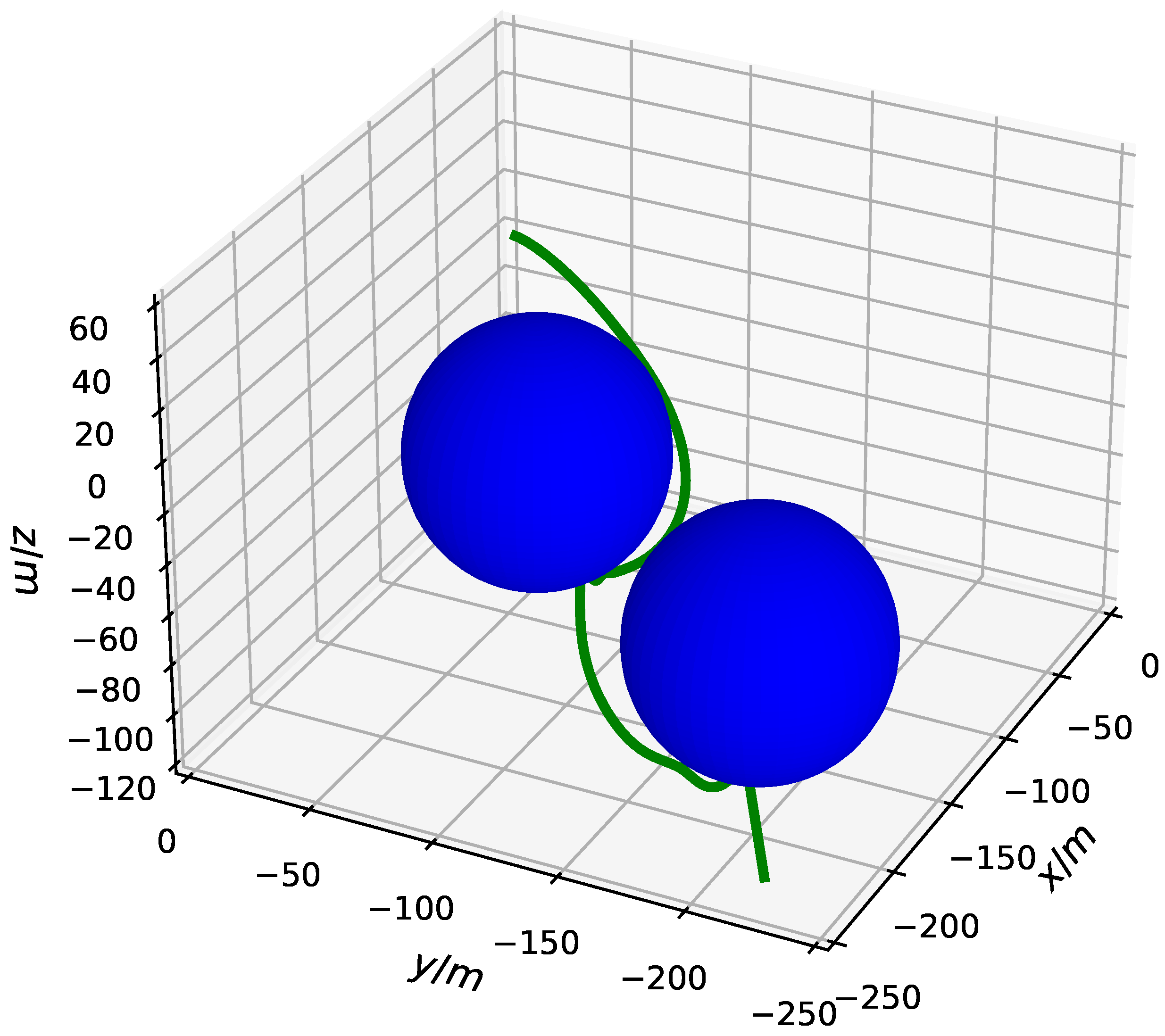
The simulation results using the second order sliding mode terminal controller are shown as follows. Figure 1 and Figure 2 show the three-dimensional motion trajectory of the spacecraft relative to the obstacle from two perspectives, respectively. The blue shadow sphere in the figure indicates the spatial influence range of the obstacle, and the radius of each sphere is set at $50\mathrm{m}$. The spacecraft approaches from the starting point to the end point and finally reaches the desired position to form a configuration and maintain it.

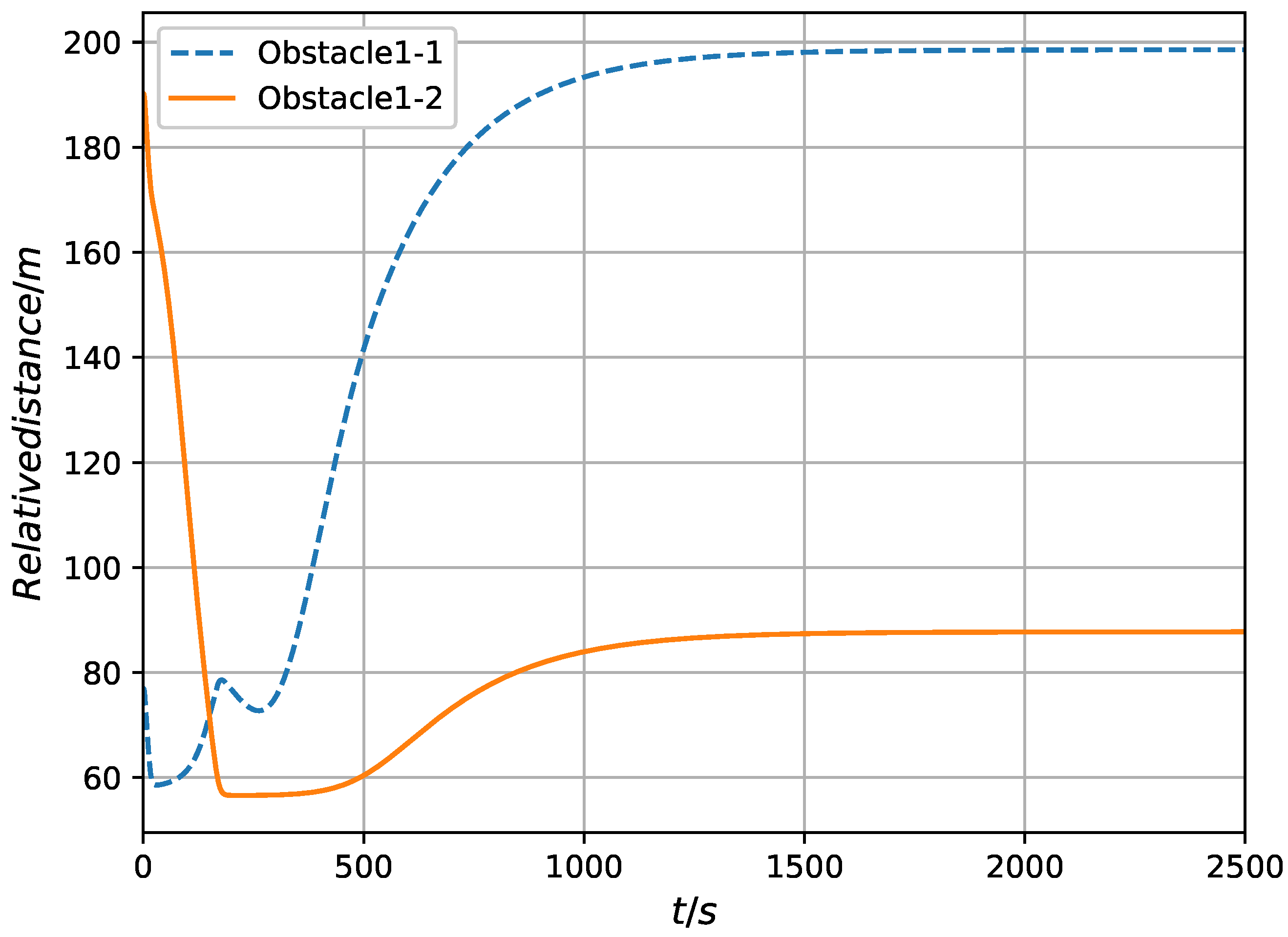
Figure 3 and Figure 4 represent the relative distance between the spacecraft and each obstacle. When the spacecraft approaches the obstacle at nearly $50\mathrm{m}$, the distance expands rapidly, keeps away from the obstacle or close to the edge of the danger area of the obstacle, and approaches the expected position. The distance in the whole process is greater than $50\mathrm{m}$, indicating that the spacecraft avoids the collision danger area of the obstacle. It can be understood that there is no collision between the spacecraft and the two obstacles.

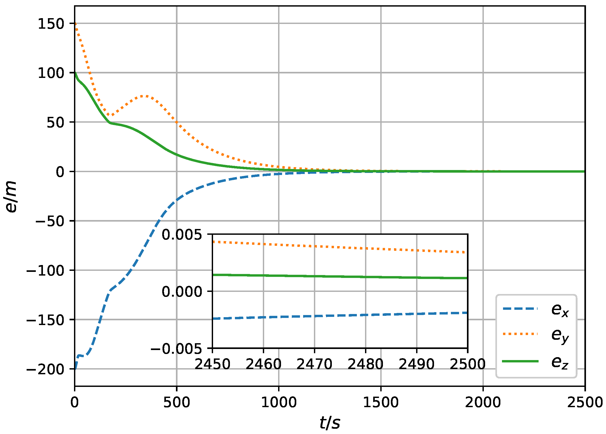
Taking Sat1 as an example, it can be seen that the spacecraft reaches the desired state after avoiding obstacles to achieve the purpose of final control. It can be seen from Figure 5 that the obstacle avoidance time is about 1000 s. Then, the steady-state error of configuration maintenance is within 0.005 m. It can be seen from Figure 6 that the controller output increases when the spacecraft is close to the obstacle.

In order to facilitate the comparison of the effects of this method, the following traditional sliding mode controller designed by the exponential approach law is used for numerical simulation of obstacle avoidance:

$$\begin{array}{cc}\hfill \dot{s}& =k\Omega +\ddot{e}\hfill \\ \hfill u& =-k\left(\frac{\partial {\nabla }_{\rho }\phi }{\partial \rho }\right)\dot{\rho }-k\left(\frac{\partial {\nabla }_{\rho }U}{\partial {\rho }_d}\right){\dot{\rho }}_d-k\sum _{i=1}^n\left(\frac{\partial {\nabla }_{\rho }{U}_{{\rho }_i}}{\partial r_{o,i}}\right){\dot{r}}_{o,i}\hfill \\ \hfill & -{\lambda }_{1}s-{\lambda }_{2}sgn{\left(s\right)}^{\alpha }-f(\rho ,v)+r_d\hfill \end{array}.$$

(44)

The initial parameters of the simulation are consistent with the above. The parameters of the traditional sliding mode controller (SMC) are designed as

Table 4. SMC controller parameters.

k	${\mathit{\lambda }}_1$	${\mathit{\lambda }}_2$	$\mathit{\alpha }$
$diag(0.5,0.3,0.4)$	$diag(0.3,0.3,0.3)$	$diag(0.3,0.3,0.3)$	$0.5$

:

The simulation results are as Figure 7, Figure 8, Figure 9 and Figure 10:

It can be seen that when the spacecraft approaches an obstacle, the output of the controller increases significantly, and the entire process of avoiding the obstacle lasts for a long time. Compared with the traditional sliding mode control, the upper limit of the output of the control amount of the second-order sliding mode control is smaller, the duration of the control output is shorter, and the second-order sliding mode control weakens the vibration phenomenon of the controller.

The simulation results in this section show that the second-order sliding mode obstacle avoidance controller proposed by Section 3 can realize the spacecraft formation formation reconstruction task in the presence of obstacles.

5. Semi-Physical Simulation Experiment of Satellite Simulator

In order to prevent the advanced control methods of spacecraft formations from being disconnected from practical applications, it is necessary to develop control hardware and software related to simulating operation in the space environment, establish an experimental platform that can simulate satellite formation control, and study new types of practical control methods that are conducive to engineering practice. The air flotation platform is used to simulate the flight of satellites in orbit and to verify the accuracy of satellite formation modeling and the performance of the formation controller. It has flourished due to its low cost, high reliability, and wide range of applications.

In this chapter, a semi-physical simulation experiment is carried out with a satellite simulator to verify the effectiveness of the second-order terminal sliding mode spacecraft obstacle avoidance controller proposed by Section 3, and the results are analyzed.

5.1. Establishment of Satellite Simulator Simulation Environment

The simulation environment of the satellite simulator mainly includes the satellite simulator subsystem, measurement subsystem, control subsystem, and marble air floating platform. The overall schematic of the semi-physical simulation environment is shown in Figure 11, and the real scene is shown in Figure 12.

Through the coordinated networking work of the above subsystems, an experimental platform that can simulate the control of space networked satellite formations is formed. Semi-physical simulation will be carried out through the coordinated control method proposed; in theory, combined with the problems encountered in the actual experiment process and analysis, the control method will be further improved, and the advanced control method will truly be integrated with the actual control application to achieve the desired control effect.

The satellite simulator subsystem is the most important part of the test, and the components of this subsystem are shown in

Table 5. Satellite simulator subsystem components.

Type of Component	Component Name
	Industrial control computer
	Digital output card
	Wireless network card
Control and communication components	Wireless router
	Solenoid valve
	Air jet nozzle
	Rigid body reflecting ball
	High-pressure composite gas cylinder
	Cylinder terminal connector
	Filters
	High-pressure regulating valve
Air supply components	High-pressure barometer
	High-pressure gas pipeline fittings
	Low-pressure regulating valve
	Low-pressure barometer
	Low-pressure gas pipeline fittings
	Lithium ion battery
	DC-DC cable
Power supply components	Plug for connection
	Air switch
	Electric wire

.

The satellite simulator is connected with a rigid reflecting ball to establish a rigid body. The vision camera captures the shape of the rigid body and calculates the position and attitude information of the satellite simulator. The host computer communicates with the communication component of the satellite simulator through the WiFi network to obtain the real-time position and attitude information of the satellite simulator and display it.

The control subsystem uses the control law to calculate the reference trajectory and transmits the desired trajectory to the satellite simulator through the Wifi signal. The lower computer of the satellite simulator controls the jet nozzle through the internal feedback loop to air injection so that the satellite simulator can track the reference trajectory in real time, to complete the control goal. The control flow of the satellite simulator is shown in Figure 13.

It is worth stating that the reference trajectory is a set of time-discrete position data, and the time interval is the jet period of the satellite simulator jet nozzle.

The jet nozzle distribution of the satellite simulator is shown in Figure 14. The satellite simulator has a total of 8 jet nozzles. The air injection of the jet nozzle is controlled by controlling the switch of the solenoid valve, so that the force in both x and y directions and the torque in z direction can be provided.

Using the assembly method of the above-mentioned control actuator, the three-degree-of-freedom movement can be easily and effectively simulated, including two shifts in the horizontal plane and rotation around the z-axis. This satellite simulator can verify the coupled motion process of attitude and trajectory. This experiment is mainly used for obstacle avoidance verification of the two-position plane. The rotational movement around the z-axis only needs to maintain the angular orientation.

5.2. Validation of the Controller

In order to enhance the credibility of the test, the parameters of the obstacle avoidance controller are selected in accordance with Table 3. The artificial potential function parameters are shown in

Table 6. Artificial potential function parameters.

P	M	${\mathit{N}}_{\mathit{i}}$	${\mathit{\sigma }}_{\mathit{i}}$	${\mathit{\psi }}_{\mathit{i}}$
$0.012\times diag(1,1,1)$	$diag(0.8,0.6,0.4)$	$diag(15,15,15)$	10	$5\times {10}^3$

. The initial position, desired position, and radius settings are shown in

Table 7. Initial/desired position selection (mm).

Initial State	Position of Obstacles	Desired State
${\rho }_1={[1400,-1400]}^T$	$r_{o,1}={[-1000,-100]}^T$	${\rho }_{d1}={[1818,1915]}^T$
${\rho }_2={[100,-1400]}^T$	$r_{o,2}={[900,1000]}^T$	${\rho }_{d2}={[170,1887]}^T$
${\rho }_3={[-1100,-1400]}^T$	$r_1=r_2=800$	${\rho }_{d3}={[-1247,1836]}^T$

.

The marble air floating platform consists of two $6\mathrm{m}\times 3\mathrm{m}$ marble pieces stitted into a complete $6\mathrm{m}\times 6\mathrm{m}$ platform; the satellite simulator, through air injection, makes the air foot and marble air floating platform produce a layer of stable air film, making the satellite simulator in the floating microgravity produce a frictionless state and a simulation of the space weightlessness environment, to achieve three degrees of freedom of free movement without external force.

Through the coordination of the above subsystems, an experimental platform is constructed to simulate the formation control of space network satellites, so that the effectiveness of the proposed control algorithm can be experimentally verified.

The controller parameters are set as shown in the following table.

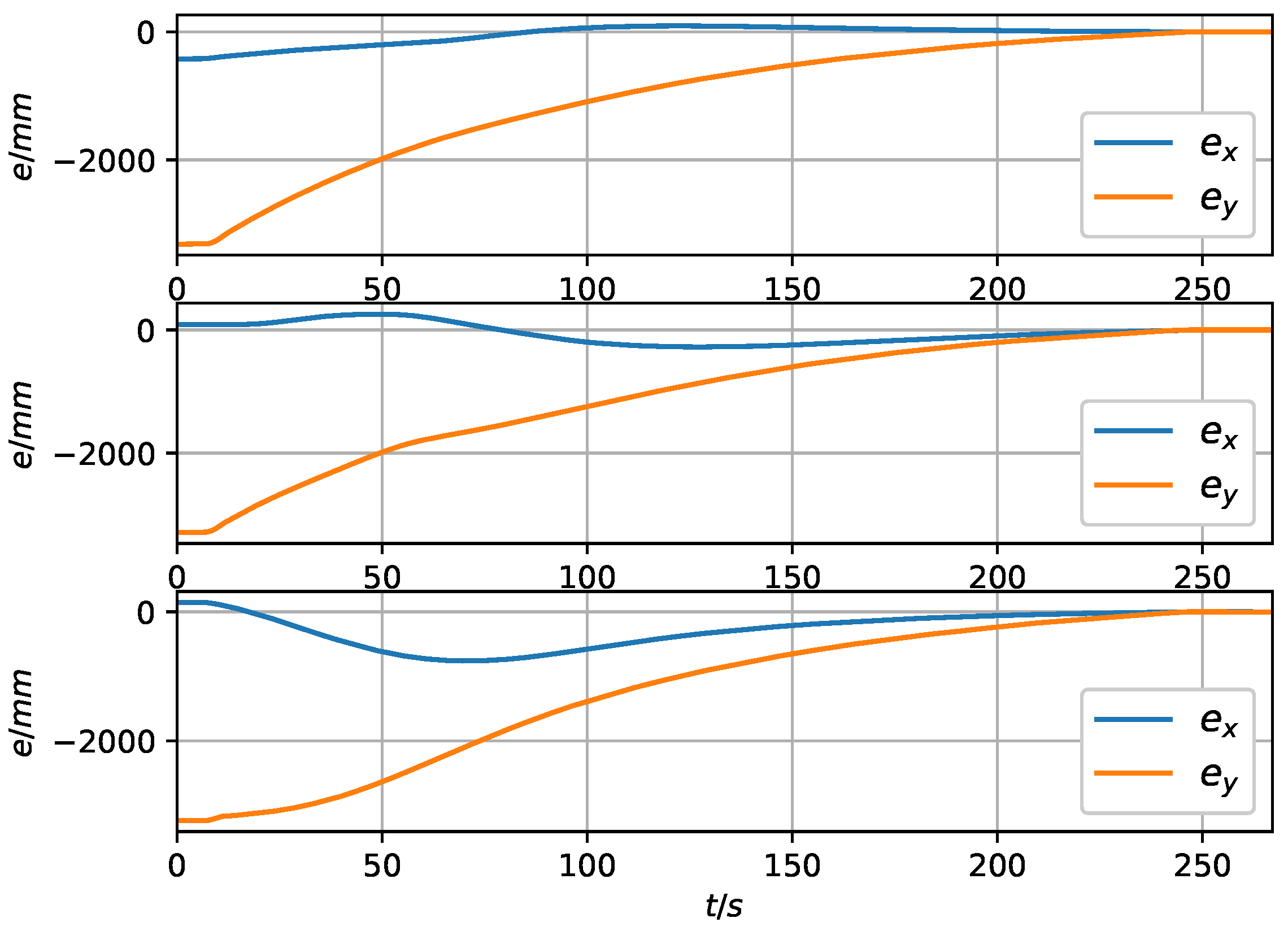
The obstacle avoidance motion trajectory of the satellite simulator and the relative motion error are shown in Figure 15 and Figure 16. Figure 17 is a video screenshot during the obstacle avoidance process of the satellite simulator. The tracking error between the satellite simulator and the desired position at the next time instant is shown in Figure 18. It can be seen that under the action of the second-order terminal sliding mode obstacle avoidance controller proposed in Section 3, the satellite simulator can complete the control task in the predetermined situation.

In the process of carrying out control experiments, due to limited engineering technologies such as manufacturing, processing, and assembly, the thrust output of the simulator has large installation errors and output errors, and the quality and moment of inertia of the simulator are subject to uncertain changes with the consumption of working fluid. At the same time, there are various external disturbances such as friction in the experimental environment, resulting in inevitable differences between the experimental results and the numerical simulation results. For the numerical simulation results, it is necessary to further improve the accuracy of the modeling based on the experimental results, fully consider the uncertainty factors such as changes in internal parameters of the system and external interference, and study a robust control algorithm similar to this method to reduce the sensitivity to interference. At the same time, we must also consider the limitations of hardware computing power and practical application. For example, improper handling of the integration link in the control algorithm will cause the experimental control process to diverge and produce unpredictable hazards.

In summary, the second-order terminal sliding mode obstacle avoidance controller proposed in this paper is effectively verified by the test of the satellite simulator.

6. Results

This paper first combines adaptive control with second-order terminal sliding mode control and designs an adaptive second-order terminal sliding mode controller (SOTSMC) to solve the uncertainty control problem of the system.

Then, flight safety issues such as obstacle avoidance and anti-collision of satellite formations during configuration initialization or reconstruction are considered; the artificial potential function guidance is combined with the adaptive second-order terminal sliding mode controller; and a navigation controller is designed so that the formation can achieve high-precision target tracking, configuration initialization, configuration reconstruction, and other tasks at the same time, to enable the avoidance of obstacles with measurable position and speed. Numerical simulation analysis shows that the second-order sliding mode control proposed in this paper has the ability to avoid obstacles after combining with the navigation algorithm. Compared with the traditional sliding mode control, the control accuracy is improved and the vibration phenomenon of the controller output is significantly weakened.

Finally, using the three-axis satellite simulator, the application of the control algorithm proposed in this paper in obstacle avoidance scenarios was physically tested. Based on the test results, combined with numerical simulation and actual situation, a comparative analysis is made to verify the effectiveness of the controller and the engineering application value. Although limited by the allocation of hardware resources and the influence of some non-ideal test environments, some control processes in the actual application results do not achieve the ideal results, but the physical tests have also further combined the theory of the controller with the actual engineering application, highlighting some practical problems that were missed in the theoretical analysis, so that in the future controller design process, theoretical research can make targeted progress towards solving actual control problems.

On the basis of the research of this thesis, in-depth research is required from the following aspects in the follow-up.

The integration process in the second-order sliding mode control weakens the controller vibration problem caused by the symbol term and causes significant harm to actual engineering applications. Experimental verification and analysis show that when the manufacturing accuracy of the controller is not high, there is an error between the actual output of the controller and the nominal output. The error will gradually accumulate due to integration during the control process, affecting the subsequent control process.Therefore, it is necessary to further study the integration saturation and controller fault tolerance of the second-order sliding mode control in practical applications in the future.

In the process of obstacle avoidance and navigation, if the output amplitude of the controller is limited, and the initial speed of the formation members is high, the speed cannot be reduced to zero in time before reaching the dangerous area, so there will be a risk of collision. Therefore, the output saturation of the controller needs to be further considered in the design process of the controller. At the same time, it is necessary to further consider the research on the control algorithm of the controlled object under drive conditions.