Abstract
In this paper, we propose a methodology for computing the square root of a complex number based on a piecewise linear (PWL) approximation method. The proposed method relies on a software-based segmentor that automatically divides the three real square root functions used in complex square root computation into the fewest segments with a predefined fractional bit width and maximum absolute error (MAE). The coefficients, including the start point, end point, slope and y-intercept of each segment, are stored for use in the implementation of the hardware design. The proposed fully pipelined circuit is coded in the Verilog hardware description language (HDL). The results of synthesis in TSMC (Taiwan Semiconductor Manufacturing Company) 65-nm CMOS technology show that our design achieves savings of 64.21% in area, 16.67% in delay and 65.08% in power compared to the existing methods. Moreover, implementation results on an FPGA (Field-Programmable Gate Array) platform (XC7Z020-CLG400) show that the proposed design reduces the number of LUTs by 29.38%, delay by 28.57% and power consumption by 53.47%.
1. Introduction
Square root computations of complex numbers are commonly used in principal numerical computations [1], signal processing algorithms [2], quantum defect theory [3], and wave propagation [4]. When implemented in software, the complex square root operation requires a long execution time, leading to difficulty in meeting requirements for high speed and low latency. Therefore, various kinds of hardware implementations have been proposed for computing complex square roots, such as the digit-recurrence algorithm [5,6,7], 2D cubic convolution [8], and the coordinate rotation digital computer (CORDIC) method [9,10,11].
The digit-recurrence algorithm, which is commonly used in real square root computation, was applied for the computation of the square root of a complex number for the first time in [5]. Subsequently, Wang et al. designed a complex square root computation for field-programmable gate array (FPGA) implementation using a radix-4 digit-recurrence algorithm [6]. A radix-16 digit-recurrence algorithm was later proposed to reduce the number of iterations [7]. Additionally, a 2D interpolation method was introduced to reduce the size of the prescaling lookup tables (LUTs). Various numbers of iterations can be employed in the digit-recurrence algorithm to achieve different levels of precision. However, the execution of multiple iterations can lead to high latency. Although a high-radix digit-recurrence approach reduces the number of iterations needed, it increases the complexity of each iteration module. Ref. [8] proposed an FPGA design for a complex square root unit using 2D cubic interpolation. The above architectures all contain recurring modules; specifically, digit recurrence reuses each iteration unit, and interpolation reuses a multiply-and-accumulate unit. Therefore, obtaining a valid output requires multiple clock cycles. Ref. [7] applied CORDIC to implement the computation of a fixed-point complex square root. Ref. [9] eliminated the need for hyperbolic CORDIC in [7]. Later, Ref. [9] reused circular CORDIC to reduce the area occupied and adopted a double pipeline concept to reduce latency. Similar to the architectures of the digit-recurrence algorithm and the interpolation method, such circuit reuse necessitates multiple clock cycles to obtain a valid output. Ref. [11] proposed a CORDIC-based very-large-scale integration (VLSI) architecture design methodology for complex square root computation that is independent of angle computation. The fully pipelined structures (yielding a valid output in every cycle) based on the CORDIC algorithm that are presented in [10,11] perform well in terms of throughput, but are weak in latency because of their numerous iterations.
In piecewise linear (PWL) approximation, a nonlinear function is divided into several segments. In each segment, the nonlinear function is approximated by a linear function. Previously, PWL methods have been proposed for the implementation of specific unary functions, without generality. Ref. [12] proposed a universal PWL method relying on a software-based segmentor with the self-adaptive ability to choose the smallest number of segments under the constraint of a controllable maximum absolute error (MAE). Based on [12], a piecewise linear approximation computation (PLAC) method was subsequently proposed that made use of an optimized segmentor, a novel quantizer and a nonredundant hardware architecture [13]. Later, PLAC was applied in a VLSI architecture for calculating the Nth roots of floating-point numbers [14]. The absolute advantage of [14] when compared with state-of-the-art architectures indicates that a PWL has natural advantage in terms of hardware overhead, especially latency, when the computation does not require high precision. Recently, a complex-valued neural network (CVNN) was proposed to improve the performance of gradient regularization [15]. In the CVNN method, low latency and high hardware efficiency are pursued rather than high precision in computations involving complex numbers.
In this article, we propose a PWL-based architecture for computing the square root of a complex number. The contributions of this paper are listed as follows.
- This is the first study in which a PWL method has been applied to implement the computation of the square root of a complex number in pursuit of low latency.
- The complex square root computation is decomposed into several substeps involving three real square root functions. A software-based segmentor approximates these real square root functions using the fewest possible segments while meeting the specified requirements of a predefined fractional bit width and MAE.
- In accordance with the fractional bit width of the slope defined in the segmentor, the bit width of the multipliers is reduced to save hardware overhead. Additionally, the multipliers are implemented with a two-stage pipelined architecture to reduce the critical path.
- Because of the usage of the state-of-the-art PWL method and a formula with a simple computational flow, our design has a significant advantage in delay. In addition, because the front part of the circuit is shared between the real and imaginary parts of the computation, the proposed architecture has an absolute advantage in hardware overhead.
2. Theoretical Background
2.1. PWL Method
In the PWL method, a nonlinear function is divided into multiple segments. For the calculation of the complex square root, the real square root functions used are nonlinear functions calculated using the PWL method. For the segment with index i, the input x belongs to the range . When , the nonlinear function is approximated by a linear function , where and are the slope and y-intercept, respectively.
Two factors affect the approximation precision of the PWL method. The first is the method used to generate the slope and y-intercept of each linear segment. In previous methods, the generation of the slope and y-intercept has depended on the properties of the target function. In [12,13,16], however, a method of generating the slope and y-intercept was proposed that is completely independent of the properties of the target function. In addition, the performance of this generation method was proven. In this paper, we adopt this latter generation method for the slope and y-intercept. The other factor influencing the approximation precision of the PWL method is the width of each segment. The use of smaller segments increases the approximation precision, but simultaneously increases the number of segments, leading to considerably higher area consumption for coefficient storage.
2.2. Precision Criteria
For the evaluation of computation precision, the MAE is defined as
Additionally, the average absolute error (AAE) is defined as
In the above expressions, PA and PE denote the approximate and exact values, respectively.
3. Proposed Methodology
In this section, we propose a segmentor coded in MATLAB for the complex square root function based on the optimized segmentor for nonlinear unary functions presented in [16].
3.1. Optimized Segmentor for Computing the Real Square Root
The segmentor in [16] was proposed based on the PLAC method in [13] by incorporating quantization operations and optimizing the y-intercept after quantization. Implementation results reveal that a logarithmic converter based on the method in [16] shows improvements over the one in [13] in all respects. Moreover, this segmentor can be easily generalized to the implementation of other nonlinear functions, such as the real square root functions involved in the complex square root computation. The segmentor for computing the real square root, for which readers can refer to [16], is not described in this paper to keep the paper reasonably concise. In [16], qw is the fractional bit width of the intermediate data used in the computation. However, the multipliers in [16] have a large hardware overhead. To reduce the bit width of the multipliers, we introduce a new parameter kw to represent the fractional bit width of the slope. The final value of kw is smaller than qw.
3.2. Proposed Segmentor for Computing the Complex Square Root
The complex square root function is computed as follows:
where
In Equations (3) and (4), there are four real square root functions. However, is shared between the real and imaginary parts. Therefore, only three real square root functions need to be calculated using the PWL method. The errors of the real and imaginary parts of the complex square root are determined from the errors of the real square roots calculated using the PWL method. That is, the errors of the real and imaginary parts will be smaller if the errors of the real square roots are smaller. and are the calculated and predefined MAEs, respectively, of the complex square root. is used to constrain the MAE of the hardware implementation and the value of after segmentation. The value of after segmentation is equal to the MAE of the hardware implementation and must be no larger than . Accordingly, the segmentor must modulate the MAEs of the real square root functions calculated with the PWL method to ensure that is no larger than . To this end, in the segmentor for computing the real square root, is used to constrain the MAE of each real square root function calculated with the PWL method. The segmentor for the real square root computation divides the inputs of each real square root function into the fewest number of segments possible while ensuring that the calculated MAE of each real square root function is no larger than . Meanwhile, the start points, end points, slopes and y-intercepts of the segments are stored for the design of the hardware implementation. Before the segmentor is applied, the values of kw and qw are predefined to determine the fractional bit widths of the slope and intermediate data, respectively. In addition, is used to constrain the MAE of the circuit (). In other words, is guaranteed to be smaller than a predefined MAE. The proposed segmentor for the complex square root function, as illustrated in Figure 1, performs the following steps:
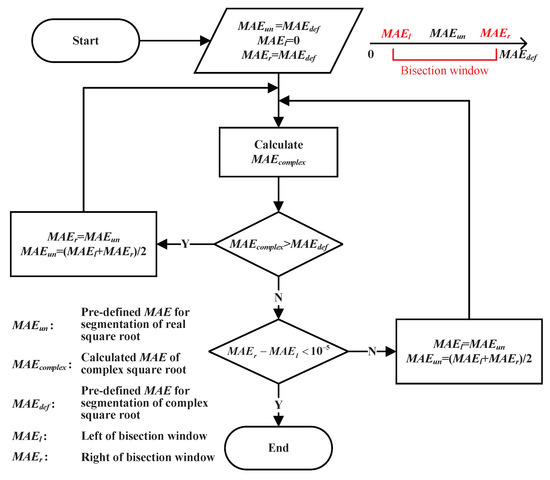
Figure 1.
Calculation flowchart of the segmentor for the complex square root function.
1. Initialization. As seen from Equations (3) and (4), the computations of the real and imaginary parts of the complex square root function each involve two real square root functions. The MAEs of these real square root functions will inevitably be smaller than that of the complex square root function. Therefore, is initialized as because the final value of must be smaller than . To reduce the execution time of the segmentor, the bisection method is used. is always located at the center point between the left and right edges of the bisection window, denoted by and , respectively. The length of the bisection window is reduced by half after each comparison of and . We use MATLAB R2019a to model the proposed segmentor. and are initialized as 0 and , respectively, to establish the largest possible range for the value of .
2. calculation. In this step, the computation of the hardware circuit is completely simulated in software. is calculated in accordance with the simulated results and exact values. This step is introduced in detail in Section 3.3.
3. Conditional judgment. If is larger than , then is too large to satisfy the predefined for the complex square root function. Therefore, should be reduced by shifting to and then moving to the center of the new bisection window. Then, the process returns to step 2 to start a new loop. If is smaller than , then the current value of constraining the segmentation of the real square root function is sufficiently small to achieve the precision specified by . At this time, the gap between the left and right edges of the bisection window is compared against a small value, defined as in our design. If this gap is not sufficiently small, can be further enlarged by shifting to and then moving to the center of the new bisection window. Then, the process returns to step 2 to start a new loop. Once the gap is found to be sufficiently small, the most appropriate value of is considered to have been found, and this value will be used to segment the real square root functions.
3.3. Calculation of
As stated in Section 3.2, the calculation of relies on the simulation of the hardware circuit. The hardware is simulated with a finite fractional bit width of
or
where df and dr are the truncated and rounded versions of d, respectively. The quantification operation based on Equation (5) results in the maximum error of , but does not incur any extra hardware overhead. In contrast, the quantification operation corresponding to Equation (6) consumes additional hardware resources, but incurs only a small precision loss of .
The real and imaginary parts of the input both lie in the range (1, 2), the same as in [8]. The input is discretized as and , where iw is the fractional bit width of the input, set to 10 in our design. The pseudocode of the algorithm for calculating is presented in Algorithm 1, and the corresponding calculation flow is illustrated in Figure 2. In the Simulation of the Hardware Circuit part, Tr(d, qw) and Ro(d, qw) are used to express the truncation operation in Equation (5) and the rounding operation in Equation (6), respectively. On line 1, is calculated considering the truncation operation. On line 2, the segmentor for the real square root function is used with the real-time computed input range of the PWL function. On lines 5 and 9, the segmentor also uses the real-time computed values based on the PWL method to minimize the computational burden. Once the start point, end point, slope and y-intercept, denoted by , , and , respectively, have been obtained, (denoted by SR) is calculated using the PWL method with the truncation operation of . The value of R is compared against the start and end points of all segments to determine the index of the segment to which it belongs, . Then, is computed, also considering the truncation operation. Similar to lines 2 and 3, lines 5 and 6 calculate . The real part of the complex function calculated via the PWL method, PA, is obtained with the rounding operation to a fractional bit width of iw. Lines 8 to 11, which calculate the imaginary part of the complex function, follow a logic similar to that of lines 4 to 7 for the computation of the real part. For the calculation of , the exact values of the complex square root, EV, are calculated using the built-in MATLAB function. The MAE of the complex output, , is defined as the maximum MAE between the real and imaginary parts and is calculated on lines 11 to 15.
| Algorithm 1: Proposed segmentor. |
Input: , , , Output: /* Simulation of Hardware Circuit: */ 1 ; Traverse all values of i and j 2 3 ; Traverse all values of i and j 4 ; 5 ; 6 Traverse all values of i and j 7 ; 8 ; Traverse all values of i and j 9 ; 10 ; Traverse all values of i and j 11 ; /* Calculation of : */ 12 ; Traverse all values of i and j 13 ; 14 ; 15 ; 16 ; 17 |
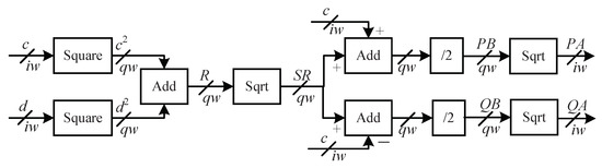
Figure 2.
Calculation flowchart of the pseudocode in Algorithm 1. The symbols qw and iw denote the fractional bit widths. Sqrt denotes the square root calculated using the PWL method in our design.
3.4. Parameter Selection
The execution time of the software-based segmentor is approximately 11 seconds using a Dell XPS 13 laptop with an Intel(R) Core(TM) i7-10710U CPU and 16 GB of RAM. The execution time depends on the performance of the computer used to model the proposed segmentor and is unrelated to the performance of the hardware implementation of the complex square root calculation.
In our design, the fractional bit widths of the input and output are both set to 10. To achieve accuracy within 1 ulp, is defined as to ensure that the MAEs of the circuit for the real and imaginary parts are both smaller than .
In addition to the predefined maximum absolute error , the fractional bit widths of the slope and other intermediate data, denoted by kw and qw, respectively, need to be predefined. The segmentor automatically divides the three real square root functions used in the complex square root computation into the fewest possible segments given the predefined values of kw, qw and . It is obvious that smaller values of kw and qw will lead to a larger number of segments. In the parameter selection step, we first set kw to be the same as qw. Different qw values lead to different numbers of segments, as shown in Figure 3a. The error of the proposed method consists of two components: the segmentation error and the quantification error. As an approximate computing method, the PWL method is the origin of the segmentation error. The segmentation error decreases with an increasing number of segments. The quantification error is introduced by the truncation and rounding operations in the circuit. In the simulator, we use Equations (5) and (6) to simulate these two operations in the circuit. Thus, the MAE calculated by the simulator also contains both errors. Smaller fractional bit widths (qw and kw) will result in a larger quantification error. However, the sum of the two errors must be no larger than ( in our design). When kw/qw changes from 12 to 18, the quantification error decreases; in turn, the number of segments can decrease from 36 to 30 because a larger segmentation error can be accommodated. Thus, the number of segments slowly decreases with increasing qw. Notably, however, the segmentor cannot converge when qw is smaller than 12. Therefore, qw is set to 12 and held unchanged for the selection of kw. Figure 3b shows how the number of segments varies with various values of kw. The error introduced by the quantification of the slope is part of the quantification error. In Figure 3b, the values of kw are scanned for set values of qw ranging from 12 to 18. Because we select 12 as the value of qw, we focus on the curve corresponding to the case in which qw is set to 12. With larger values of kw, the quantification error and the number of segments both decrease. As seen from Figure 3b, when the value of kw is smaller than 6, the segmentation error is limited to a small value. Thus, the number of segments can be greatly reduced from 232 to 73 when kw changes from 5 to 6. However, the segmentation error of the PWL method becomes much larger when kw is larger than 6. Thus, the number of segments becomes saturated when kw is larger than 6. To optimize the bit width settings, the end point of the flat part of the curve in Figure 3b is selected. In accordance with the above selection method, qw and kw are set to 12 and 7, respectively. The values of qw and kw mainly affect the bit widths of the computing resources. Thus, larger qw and kw values would lead to an increase in delay. Meanwhile, the number of segments output by the segmentor mainly affects the required storage size. Based on these considerations, in practical applications, the values can be selected in accordance with the requirements of the hardware implementation.
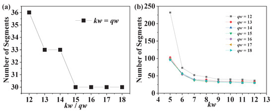
Figure 3.
(a) The relationship between the number of segments and kw or qw when kw is equal to qw. (b) The relationship between the number of segments and kw.
4. Hardware Implementation and Comparison
4.1. Implementation Results and Comparison
We replicated the architectures in [8,10,11] with the same fractional bit widths of the input and output and a precision comparable to that of our design. We list the parameters and errors in Table 1. The three replicated architectures and our design were all coded in the Verilog hardware description language (HDL) and synthesized using Synopsys Design Compiler (DC) in TSMC 65-nm CMOS technology. The synthesis results are listed in Table 2. Moreover, we implemented the designs in Vivado 2017.4 based on a Xilinx Zynq-7000 SoC XC7Z020-CLG400 FPGA. In Vivado, the synthesis and implementation steps are successively executed. Then, the implementation results are reported by Vivado. The Vivado implementation results are listed in Table 3.

Table 1.
Error comparison of our design and existing designs.
Table 2.
Performance comparison of our design and existing designs based on the results when synthesized in TSMC 65-nm CMOS technology.
Table 3.
Performance comparison of our design and existing designs based on the results when implemented in Vivado based on a Xilinx Zynq-7000 SoC XC7Z020-CLG400 FPGA.
4.2. Details of Hardware Implementation
The hardware architecture of our design is illustrated in Figure 4, with the sel and PWL parts shown in Figure 5. The hardware architecture of our design exhibits good correspondence with the simulation of the hardware circuit in the segmentor illustrated in Algorithm 1. In our design, the fractional bit width of the intermediate data is 12, in accordance with the selection process described in Section 3.4. The fractional bit widths of the input and output are again set to 10. To shorten the critical path, all multipliers are implemented with a two-stage pipelined architecture. One of the two 11-bit multipliers calculating the squares of the two inputs is implemented with 4 6-bit multipliers and one 22-bit adder. Each multiplier in the PWL module occupies 2 multipliers and one 22-bit adder.
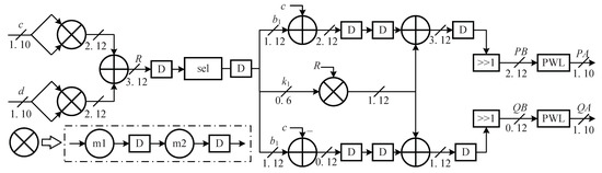
Figure 4.
Hardware architecture of the proposed design for the computation of the complex square root function.
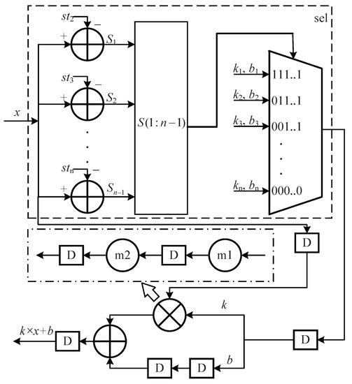
Figure 5.
Hardware architecture of the PWL and sel parts in Figure 4. The symbols with the format in the comparator indicate the start point of the segment. The symbols indicate the sign bit of the comparator.
Initially, two multipliers concurrently calculate the squares of the real and imaginary parts of the input. An adder is used to obtain the sum of these two squares, , as shown on line 1 in Algorithm 1. Once R has been located in its corresponding segment, the real part of the input, x, is both added to and subtracted from the y-intercept of the selected linear function without waiting for the results of . Concurrently, a multiplier with a two-stage pipelined architecture is used to calculate . Then, the output of the multiplier is added to and in parallel. After a rightward shift by one bit, PB and QB in Algorithm 1 are calculated. The above circuit calculates the real and imaginary values in parallel. It has the same results as lines 2–4 and 8 of Algorithm 1, but the steps here are different because of the parallelization of the calculation of with the addition/subtraction between and x. Finally, two PWL circuits are simultaneously employed to calculate and , corresponding to lines 6 and 10 in Algorithm 1. Before the output is returned, it is truncated to 10 fractional bits after adding one () to the 11th fractional bit.
In total, our design includes five two-stage multipliers, seven adders, 49 comparators and three multiplexers. In addition, the segmentor outputs the start point, end point, slope and y-intercept of each segment. As shown in Figure 5, the start points of the second-to-last segments are used as the inputs to the comparators. The slopes and y-intercepts of all segments are selected by the signs of the comparators. If the number of segments is n, then n − 1 start points, n slopes and n y-intercepts are stored on chip. Three real square roots are calculated via the PWL method according to lines 2, 5 and 9 in Algorithm 1. The total number of segments (NS) is 52. Thus, the required storage space is bits. As shown in Figure 4, all multipliers in our design are implemented with a two-stage pipelined architecture. Figure 5 shows the implementation of each PWL circuit requires four clock cycles. As a result, the total number of clock cycles required by the proposed architecture is 11.
To compare our design with the architectures in [8,10,11], we replicated these three hardware implementations with errors at the same level as in our design. The synthesis results are listed in Table 2. Additionally, , defined as , is introduced as a composite indicator of hardware implementation performance. The fractional bit width of [8] was set to 11. The number of iterations and the fractional word length in the replicated architectures of [10,11] were set to 11 and 14, respectively. The MAE and AAE values of the circuits considered for comparison and our design are listed in Table 2. Our design shows absolute predominance in precision compared with the replicated designs of [8,10,11].
In the design of [8], the five most significant bits of the fractional part are used to generate interpolation nodes, and the other five least significant bits are used to calculate interpolation coefficients. Therefore, the size of the coefficient table is 26,840 bits, which is 17 times that of our design. In addition, there are eight multipliers, two compressors and two adders in this design. The design in [8] also requires 11 clock cycles. However, it recycles computing resources. Five clock cycles are needed to produce one valid output. In contrast, our design generates one output per cycle because it is a fully pipelined architecture. In summary, our design achieves savings of 64.21% in area, 16.67% in delay, 65.08% in power, and 89.59% in compared with [8].
In the design of [10], three kinds of CORDIC units are executed sequentially in the following order: circular vectoring mode (CV) CORDIC, hyperbolic vectoring mode (HV) CORDIC, and circular rotation mode (CR) CORDIC. To guarantee convergence, the fourth iteration is executed twice. Because the number of iterations of the CORDIC units is set to 11, the total number of clock cycles for [10] is 34. The architecture of [11] includes one CV CORDIC unit and two HV CORDIC units. Each HV CORDIC unit needs one additional iteration. The two HV CORDIC units are executed in parallel. The two multipliers for the scale factors of the CV and HV CORDIC units require two clock cycles. Moreover, the intermediate adders require two more clock cycles. Hence, the architecture of [11] requires 27 clock cycles to produce its first output. Therefore, our proposed architecture saves 23 and 16 clock cycles compared with the designs in [10,11], respectively. Each iteration in the architectures of [10,11] needs six 16-bit adders (one sign bit, one integer bit and 14 fractional bits) and three 2:1 multiplexers. In [10], two additional 16-bit adders are used in addition to 34 iteration modules. Therefore, the design of [10] consumes 206 16-bit adders and 102 2:1 multiplexers. In the hardware architecture presented in [11], three 16-bit multipliers and six 16-bit adders are required in addition to 35 iteration modules. In total, the design in [11] requires three 16-bit multipliers, 216 16-bit adders and 105 2:1 multiplexers. The synthesized results @1 GHz in Table 2 show that our design achieves area, delay, power, and savings of 79.79%, 67.65%, 64.95%, and 97.71%, respectively, compared with [10] and 81.61%, 59.26%, 69.44%, and 97.71%, respectively, compared with [11].
To more intuitively compare our design with the architectures based on the CORDIC algorithm, we implemented a circuit for complex square root computation with the same computing flow as our design in Figure 2. However, the square root computations were implemented by means of the HV CORDIC algorithm instead of the PWL method as in our design. The same HV CORDIC hardware architecture was used as in [17]. The number of iterations and the fractional bit width were set to 11 and 13, respectively. The fourth iteration must be calculated twice; thus, each HV CORDIC unit needs 12 iterations. After the iterations, the output is multiplied by the reciprocal of the scale factor to obtain the square root. In total, this architecture contains 219 adders and five multipliers. Because the real and imaginary parts are calculated in parallel, the delay of this architecture is 29 clock cycles. Our design achieves savings of 75.87% in area, 62.07% in delay, 60.47% in power, and 96.38% in compared with this architecture.
5. Conclusions, Limitations, and Future Research
In this article, we have proposed a VLSI architecture for the computation of the complex square root based on a PWL method. The segmentor for nonlinear unary functions in [16] is optimized by reducing the fractional bit width of the slopes of the linear functions to reduce the hardware overhead of the multipliers. Based on this, a segmentor for complex square root computation has been proposed and coded in MATLAB. The proposed segmentor automatically achieves the fewest possible segments to meet a specified MAE requirement given a predefined fractional bit width of the slope. Finally, based on the output of the segmentor, a fully pipelined circuit can be implemented. Comparisons of our design with existing implementations indicate that our design incurs less overhead in terms of area, delay and power while achieving higher precision.
The proposed computation flow for the complex square root is suitable for computations of different precisions. In our design, the precision is 1 ulp (unit in the last place) of 10 fractional bits. To our knowledge, the PWL method can be employed when the precision is lower than 1 ulp of 16 fractional bits. If the proposed method is used to calculate the complex square root with a precision lower than 1 ulp of n fractional bits where , in Figure 1 is set to . Otherwise, the design process is the same as that described in this article. The fractional bit widths and the number of segments must be larger if the precision is higher than that of the design in this paper. The hardware architecture in Figure 4 and Figure 5 is also suitable for different bit widths and numbers of segments. In the higher-precision situation, a piecewise higher-order polynomial approximation method should be used in place of the PWL method. The segmentor in [16] should be replaced by that in [18], which is based on a piecewise parabolic approximation method. Additionally, the hardware architecture in Figure 5 should be replaced by that in [18] to calculate the piecewise parabolic approximation method.
Notably, the proposed method is also suitable for the computation of other arithmetic operations on complex numbers with different computation flows. In accordance with the complex arithmetic formula, the calculation process in Figure 2 should be adjusted through a process similar to that for the proposed segmentor shown in Figure 1.
However, different arithmetic operations on complex numbers cannot share a unified hardware architecture based on this approach. Therefore, we will conduct additional research seeking a universal, uniform and high-performance hardware implementation for complex arithmetic.
Author Contributions
Conceptualization, Y.W. and X.L.; methodology, Y.W. and W.X.; software, Y.W. and C.H.; validation, Y.W. and X.L.; investigation, Y.W. and F.L.; data curation, Y.W. and W.X.; writing—original draft preparation, Y.W.; writing—review and editing, F.L., Y.L. (Yuanyong Luo) and Y.L. (Yun Li); supervision, Y.L. (Yun Li); project administration, F.L and Y.L. (Yuanyong Luo); funding acquisition, Y.W. and F.L. All authors have read and agreed to the published version of the manuscript.
Funding
This work was supported by the National Natural Science Foundation of China under Grant 62201234, the Natural Science Foundation of the Jiangsu Higher Education Institutions of China under Grant 21KJB510012, and the Scientific Research Foundation for the High-Level Talents of Jinling Institute of Technology under Grant jit-b-201907.
Data Availability Statement
Not applicable.
Conflicts of Interest
The authors declare no conflict of interest.
Abbreviations
The following abbreviations are used in this manuscript:
| PWL | Piecewise linear |
| FPGA | Field-programmable gate array |
| CORDIC | Coordinate rotation digital computer |
| VLSI | Very-large-scale integration |
| PLAC | Piecewise linear approximation computation |
| CVNN | Complex-valued neural network |
| Maximum absolute error | |
| Predefined MAE for the segmentation of a real square root function | |
| MAE of the complex square root computation | |
| Predefined MAE for the segmentation of a complex square root function | |
| Left edge of the bisection window | |
| Right edge of the bisection window | |
| of the circuit | |
| of the circuit for computing the real part | |
| of the circuit for computing the imaginary part | |
| Average absolute error | |
| of the circuit for computing the real part | |
| of the circuit for computing the imaginary part | |
| Fractional bit width of the slope | |
| Fractional bit width of the other intermediate data excepting the slope |
References
- Bindel, D.; Demmel, J.; Kahan, W.; Marques, O. On computing Givens rotations reliably and efficiently. ACM Trans. Math. Softw. (TOMS) 2002, 28, 206–238. [Google Scholar] [CrossRef]
- Sima, M.; Senthilvelan, M.; Iancu, D.; Glossner, J.; Moudgill, M.; Schulte, M. Software solutions for converting a MIMO-OFDM channel into multiple SISO-OFDM channels. In Proceedings of the Third IEEE International Conference on Wireless and Mobile Computing, Networking and Communications (WiMob 2007), New York, NY, USA, 8–10 October 2007; p. 9. [Google Scholar]
- Mitroy, J.; Ivallov, I. Quantum defect theory for the study of hadronic atoms. J. Phys. G Nucl. Part. Phys. 2001, 27, 1421. [Google Scholar] [CrossRef]
- Salo, J.; Fagerholm, J.; Friberg, A.T.; Salomaa, M. Unified description of nondiffracting X and Y waves. Phys. Rev. E 2000, 62, 4261. [Google Scholar] [CrossRef] [PubMed]
- Ercegovac, M.D.; Muller, J.M. Complex square root with operand prescaling. J. VLSI Signal Process. Syst. Signal Image Video Technol. 2007, 49, 19–30. [Google Scholar] [CrossRef]
- Wang, D.; Ercegovac, M.D. A design of complex square root for FPGA implementation. In Proceedings of the Mathematics for Signal and Information Processing, International Society for Optics and Photonics, Minneapolis, Minnesota, 17–19 May 2009; Volume 7444, p. 74440L. [Google Scholar]
- Wang, D.; Ercegovac, M.D. A Radix-16 Combined Complex Division/Square Root Unit with Operand Prescaling. IEEE Trans. Comput. 2012, 61, 1243–1255. [Google Scholar] [CrossRef]
- Wang, D.; Ercegovac, M.D.; Zheng, N. Design of High-Throughput Fixed-Point Complex Reciprocal/Square-Root Unit. IEEE Trans. Circ. Syst. II Express Briefs 2010, 57, 627–631. [Google Scholar] [CrossRef]
- Mopuri, S.; Acharyya, A. Low-complexity methodology for complex square-root computation. IEEE Trans. Very Large Scale Integr. (VLSI) Syst. 2017, 25, 3255–3259. [Google Scholar] [CrossRef]
- Yang, B.; Wang, D.; Liu, L. Complex division and square-root using CORDIC. In Proceedings of the 2012 2nd International Conference on Consumer Electronics, Communications and Networks (CECNet), Yichang, China, 21–23 April 2012; pp. 2464–2468. [Google Scholar] [CrossRef]
- Mopuri, S.; Acharyya, A. Low-Complexity and High-Speed Architecture Design Methodology for Complex Square Root. Circ. Syst. Signal Process. 2021, 40, 5759–5772. [Google Scholar] [CrossRef]
- Sun, H.; Luo, Y.; Ha, Y.; Shi, Y.; Gao, Y.; Shen, Q.; Pan, H. A Universal Method of Linear Approximation With Controllable Error for the Efficient Implementation of Transcendental Functions. IEEE Trans. Circ. Syst. I Regul. Pap. 2020, 67, 177–188. [Google Scholar] [CrossRef]
- Dong, H.; Wang, M.; Luo, Y.; Zheng, M.; An, M.; Ha, Y.; Pan, H. PLAC: Piecewise Linear Approximation Computation for All Nonlinear Unary Functions. IEEE Trans. Very Large Scale Integr. (VLSI) Syst. 2020, 28, 2014–2027. [Google Scholar] [CrossRef]
- Lyu, F.; Xu, X.; Wang, Y.; Luo, Y.; Wang, Y.; Pan, H. Ultralow-Latency VLSI Architecture Based on a Linear Approximation Method for Computing Nth Roots of Floating-Point Numbers. IEEE Trans. Circ. Syst. I Regul. Pap. 2021, 68, 715–727. [Google Scholar] [CrossRef]
- Yeats, E.C.; Chen, Y.; Li, H. Improving Gradient Regularization using Complex-Valued Neural Networks. In Proceedings of the International Conference on Machine Learning, Online, 18–24 July 2021; pp. 11953–11963. [Google Scholar]
- Lyu, F.; Mao, Z.; Zhang, J.; Wang, Y.; Luo, Y. PWL-Based Architecture for the Logarithmic Computation of Floating-Point Numbers. IEEE Trans. Very Large Scale Integr. (VLSI) Syst. 2021, 29, 1470–1474. [Google Scholar] [CrossRef]
- Luo, Y.; Wang, Y.; Sun, H.; Zha, Y.; Wang, Z.; Pan, H. CORDIC-Based Architecture for Computing Nth Root and Its Implementation. IEEE Trans. Circ. Syst. I Regul. Pap. 2018, 65, 4183–4195. [Google Scholar] [CrossRef]
- An, M.; Luo, Y.; Zheng, M.; Wang, Y.; Dong, H.; Wang, Z.; Peng, C.; Pan, H. Piecewise Parabolic Approximate Computation Based on an Error-Flattened Segmenter and a Novel Quantizer. Electronics 2021, 10, 2704. [Google Scholar] [CrossRef]
Disclaimer/Publisher’s Note: The statements, opinions and data contained in all publications are solely those of the individual author(s) and contributor(s) and not of MDPI and/or the editor(s). MDPI and/or the editor(s) disclaim responsibility for any injury to people or property resulting from any ideas, methods, instructions or products referred to in the content. |
© 2023 by the authors. Licensee MDPI, Basel, Switzerland. This article is an open access article distributed under the terms and conditions of the Creative Commons Attribution (CC BY) license (https://creativecommons.org/licenses/by/4.0/).