Economic Optimization Scheduling Based on Load Demand in Microgrids Considering Source Network Load Storage

Abstract

As a large number of flexible elements such as distributed power and flexible load are connected to microgrids, the economic improvement of microgrids has become an important topic through rational energy distribution. In this paper, an economic scheduling model considering the load demand for a microgrid system under the mechanism of a peak–valley tariff is proposed. A mathematical model of the microgrid components is proposed to determine the exchange power between the microgrid and main network. Meanwhile, an improved War Strategy Optimization (WSO) algorithm is proposed to investigate three scenarios: (i) without batteries, (ii) with batteries and (iii) with batteries and demand response. Additionally, demand response optimization is carried out with the Particle Swarm Optimization (PSO) algorithm and the improved WSO is compared with four other algorithms in scenario (iii). The comparison shows that the improved WSO algorithm has a better optimization performance in solving the proposed scheduling model.

1. Introduction

Microgrids are a special form of power grid structure. Distributed generation, a flexible load and an energy storing device are concentrated in a microgrid in order to realize deep and nearby utilization of distributed generation. Additionally, promoting the construction of microgrids is an inevitable choice to achieve the transformation of the energy structure and the strategic objectives of “carbon peaking” and “carbon neutralization” [1,2]. In addition, improving the economy of microgrids is also a factor to be considered during microgrid operation [3,4]. In this context, the impact of renewable energy generation intermittency on the electrical supply stability needs to be considered in depth. The active participation of consumers is a feasible scheme to improve operation efficiency by load reduction or load transfer [5,6]. Li Y. et al. presented a decision method to maximize system profits considering the real-time electricity price [7]. Wang J. et al. considered current and future industrial load control and designed a demand response scheme [8]. In addition, an integrated energy system has been developed, as electricity alone cannot meet the load need. Navin N. K. et al. established a power dispatching model to maximize the microgrid retailer profits according to time varying electricity prices [9]. Lu R. et al. proposed a valid method that provides users with incentive demand side response based on preferential roll [10].

Generally, the optimal operation strategy of microgrid systems focuses on several aspects, such as the economy, environmental protection and the line transmission power threshold [11,12,13]. Yiran Wang et al. built a stochastic multi-objective optimization model by using the maximum profit of demand response projects of electric power companies [14]. Khalili T. et al. proposed a mean shift entropy model in an independent microgrid with the goal of maximizing the benefits [15]. Huanhong Yang et al. established an optimization model of microgrid operation by taking the minimum operation cost of the day-ahead dispatching stage. In the operation process, a minimum control cost is the objective function [16]. Yongjun Yang et al. took the power purchase cost and the carbon emission penalty into consideration [17]. Meanwhile, Tengfei Ma et al. established the lowest daily operation cost model for microgrids [18].

So far, optimal scheduling models of microgrids are solved by mathematical programming methods and intelligent optimization algorithms [19,20,21]. Chen F. et al. simplified converted a scheduling model into a mixed integer linear programming problem for solving [22]. Gabbar H. A. et al. adopted the PSO algorithm to obtain the optimization power supply plan [23]. Further, Xingcui Li et al. adopted the improved PSO algorithm to generate the scheduling strategy considering the various factors in microgrids [24]. Ling Zhang et al. proposed the improved bat algorithm, which realized the optimal solution in an uncertain environment [25]. Pengyu Wang et al. used the distributed neurodynamic optimization algorithm in microgrids [26]. Shuqiang Zhao et al. combined fuzzy simulation and a neural network to build a hybrid intelligent optimization algorithm, and realized the optimized solution of a wind power storage microgrid system [27].

There have been a lot of research results on load demand response and microgrid power scheduling. However, the load optimization of demand response and the subsequent optimal scheduling of microgrids, as well as solving algorithms, still need to be further studied.

In this paper, the economic scheduling of a microgrid using renewable sources in interconnected mode is investigated. Demand response is considered with the mechanism of a peak valley tariff. A mathematical model of the microgrid’s components is proposed to determine the exchange power between the microgrid and the main network. The demand response and microgrid power scheduling are comprehensively studied in depth. Further, an improved WSO algorithm is proposed. The algorithm is used to investigate three scenarios: (i) without batteries, (ii) with batteries and (iii) with batteries and demand response. Demand response optimization is carried out with the PSO algorithm. In addition, to demonstrate the superiority of the improved WSO algorithm, a comparison with four other algorithms is performed in scenario (iv). In general, the method proposed in this paper provides the following contributions:

• The economic scheduling model considering the load demand for microgrid systems under the mechanism of a peak-valley tariff is established comprehensively;
• An improved WSO algorithm which introduces the dynamic weight factor of soldier ranking and the time sequence iteration update strategy of weak soldiers is used to solve the economic scheduling model under three scenarios.

Improving the economy of the microgrid is given priority in two levels of the load and the microgrid system in our study. The work in each section is arranged as follows. An economic scheduling model based on the demand response in microgrids is proposed in Section 2. In Section 3, the improved WSO algorithm is presented. Further, the solution results are discussed in detail in Section 4. Finally, the main conclusions from this research are drawn up in Section 5.

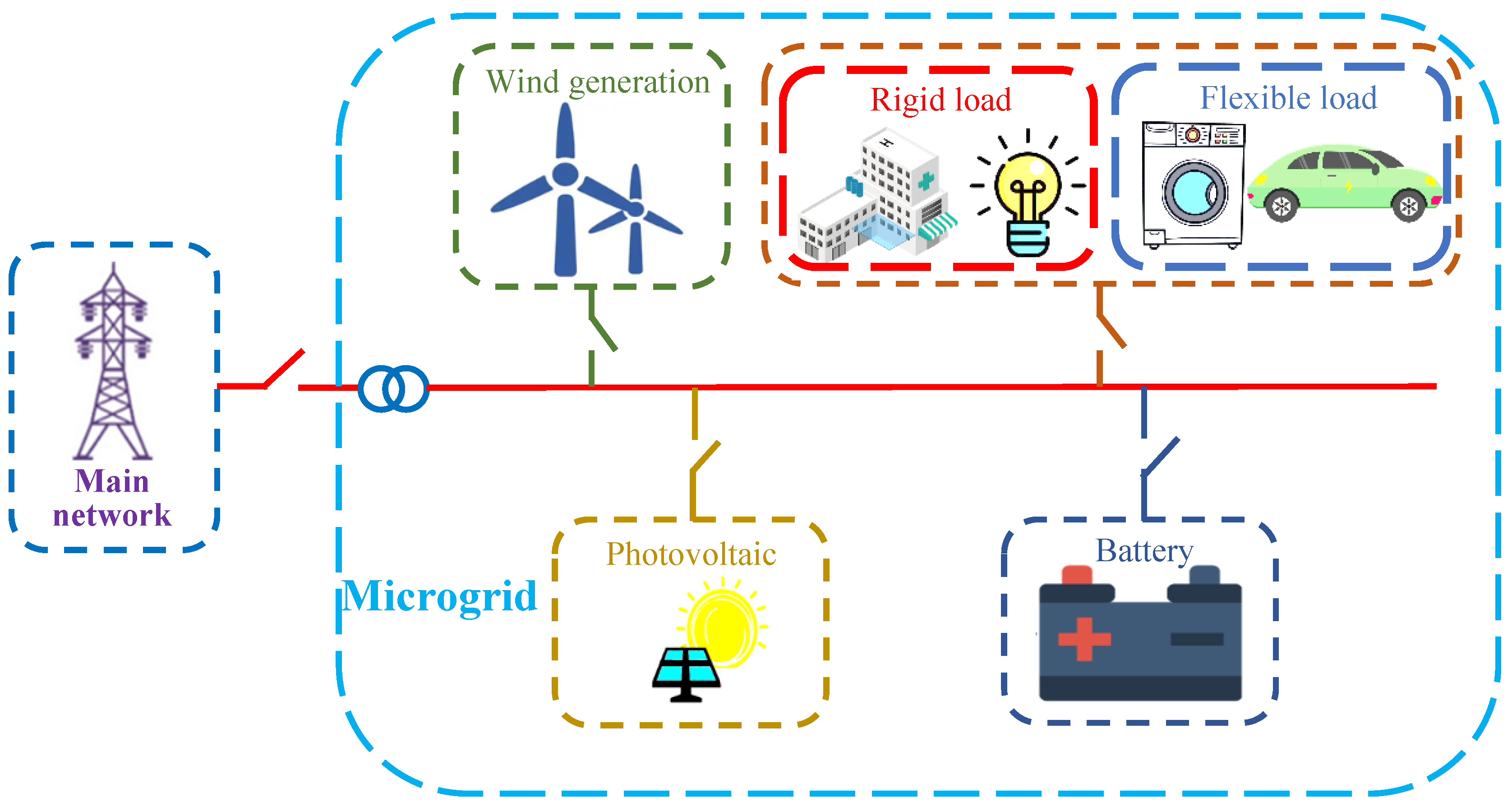
2. Microgrid Structure and Mathematical Model

2.1. Microgrid Structure

A microgrid is a small active distribution system with distributed generation, flexible loads and energy storage. Different from a traditional distribution network, the distributed generation, including photovoltaic (PV) power and wind generation (WG), and the load interact closely in the microgrid. Energy storage devices are widely developed and play a buffer role between distributed generation and electricity consumption in microgrids. In addition, the load tends to clearly fluctuate due to fine management. The load evolves into a schedulable resource and obtains the ability to participate in power scheduling by the collaboration between the microgrid and the power users. Multiple flexible resources are organically combined to form a microgrid, which is connected to the main network through a liaison line. A microgrid structure is illustrated in Figure 1. The distributed generation and the main network can achieve two-way energy exchange due to the power uncertainty of the distributed generation and the load.

2.2. Mathematical Model of Microgrid

2.2.1. Photovoltaic Generation Model

Photovoltaic generation is an indispensable part of a microgrid system. The access to PV greatly improves the independent operation capability of a microgrid due to the power output. Additionally, PV power depends on the environmental temperature and the solar radiation intensity. The PV output power is expressed by [28]

$$T_{pv}(t)=T_{en}+30G(t)/1000,$$

(1)

$$P_{pv}(t)=P_{pv,s}\frac{G(t)}{G_s}[1+k(T_{pv}(t)-T_s)],$$

(2)

where G(t) is the solar radiation value of PV, T_en and T_pv are the ambient temperature and the PV temperature, respectively. G_s is the reference value of light intensity, where the value is 1000 W/m². T_s is the reference temperature, where the value is 25 °C. P_pv is the highest test output power under the reference temperature and light intensity, P_pv is the photovoltaic cell output and k is the power temperature coefficient.

In the operation process of PV, maintenance and damage are inevitable. Therefore, the operation and maintenance costs need to be considered as follows:

$$C_{pv}={\displaystyle {\sum }_{i=1}^N\gamma P_{pv,i}\Delta t},$$

(3)

where C_pv represents the operation and maintenance costs of PV in a scheduling period, γ is a cost factor when the PV device is being repaired, i indicates the time period, N represents the number of time periods and P_pv,i represents the generated power from photovoltaics in period i.

2.2.2. Wind Generation Model

Wind generation is a form of autonomous power generation in microgrids. The power curve of WG, which depends on the wind speed, is very volatile. The wind speed is approximately consistent with a Weibull distribution, and the probability density function can be described as [29]:

$$\varphi (v)=\frac{k}{c}{\left(\frac{v}{c}\right)}^{k-1}{e}^{-{(v/c)}^k},$$

(4)

where v is the actual wind speed and k represents the wind generation shape factor. Generally, the value ranges from 1.8 to 2.8. Meanwhile, c is a scale parameter between the active wind speed and the average wind speed over a period of time.

The function relation between wind speed and WG output can be expressed by [30]

$$P_{wt}=\{\begin{array}{l}0,\hspace{1em}v<v_m\hfill \\ a{v}^2+bv+c,\hspace{1em}{v}_{in}\le v\le v_r,\hfill \\ P_r,\hspace{1em}{v}_r\le v\le v_{out}\hfill \\ 0,\hspace{1em}v>v_{out}\hfill \end{array}$$

(5)

where P_wt is the output power of WG, P_r is the rated output power, v_r, v_in and v_out are the rated wind speed, the cut-in wind speed and the cut-out wind speed, respectively, and a, b and c are the characteristic parameters.

The operation and maintenance costs of wind turbine are calculated based on Formula (6).

$$C_{wt}={\displaystyle {\sum }_{i=1}^N\delta P_{wt,i}\Delta t},$$

(6)

where C_wt represents the operation and maintenance costs of wind turbine in a scheduling period, δ is the maintenance cost factor and P_wt,i represents the generation power of wind turbine in period i.

2.2.3. Battery Model

Batteries can participate in power dispatching through power storage and power release. A battery can be used as a link between distributed generation and load. The battery reduces the negative impact of the power fluctuations caused by WG and PV. Batteries charge when renewable energy is plentiful or electricity prices are low. The charge state (SOC_t) is represented by Formula (7) [31].

$$\{\begin{array}{c}\begin{array}{cc}SO{C}_t=SO{C}_{t-1}-\frac{Q_{b,t}\cdot {\eta }_{dis}}{W_b}& Q_{b,t}\ge 0\end{array}\\ \begin{array}{cc}SO{C}_t=SO{C}_{t-1}-\frac{Q_{b,t}\cdot {\eta }_{cha}}{W_b}& Q_{b,t}<0\end{array}\end{array},$$

(7)

Further, the battery power variation can be calculated by

$$P_{bat}=W_b(SO{C}_t-SO{C}_{t-1}),$$

(8)

where ŋ_dis and ŋ_cha represent the battery efficiency under charging condition and discharging conditions, respectively. W_b is the capacity of the battery and Q_b,t represents the charge and discharge amount of the battery. A negative value indicates charge, while a positive value is discharge.

The total battery operation and maintenance cost C_bat is described by Formula (9) in a scheduling period.

$$C_{bat}={\displaystyle {\sum }_{i=1}^N\lambda P_{bat,i}\Delta t},$$

(9)

where λ is the maintenance cost factor of the battery and P_bat,i represents the battery power.

2.2.4. Power Exchange Model

The electric power exchange between a microgrid and the main network is essential as the distributed generation cannot meet the load power demand sometimes. When the distributed generation supply is insufficient, the microgrid purchases electricity from the main network. Instead, the microgrid sells electric power to the main network. The exchange power P_exc can be described as follows:

$$P_{exc}=P_{load}-P_{wt}-P_{pv}-P_{bat},$$

(10)

When P_exc is positive, the power purchase can be described as:

$$P_{buy}=P_{exc},$$

(11)

When P_exc is negative, the power sales can be described as:

$$P_{sell}=-P_{exc},$$

(12)

The power exchange cost is described by Formulas (13) and (14).

$$C_{buy}={\displaystyle {\sum }_{i=1}^N{\sigma }_{buy,i}{P}_{buy,i}\Delta t},$$

(13)

$$C_{sell}={\displaystyle {\sum }_{i=1}^N{\sigma }_{sell,i}{P}_{sell,i}\Delta t},$$

(14)

where C_buy and C_sell represent the purchase cost and income of a microgrid by power exchange in a scheduling period, respectively. σ_buy,i and σ_sell,i denote the unit price of purchases power and sold power in period i, respectively. P_buy,i and P_sell,i denote the purchase power and sale power in period i, respectively.

Parameters using in the microgrid optimization scheduling model are shown in

Table 1. Parameters of the microgrid optimization scheduling model.

Parameter	Value
Installed capacity of PV	5 MW
Installed capacity of WT	10 MW
Wb	8 MW
γ	0.78 CNY/(KW·h)
δ	0.63 CNY/(KW·h)
λ	0.2 CNY/(KW·h)

.

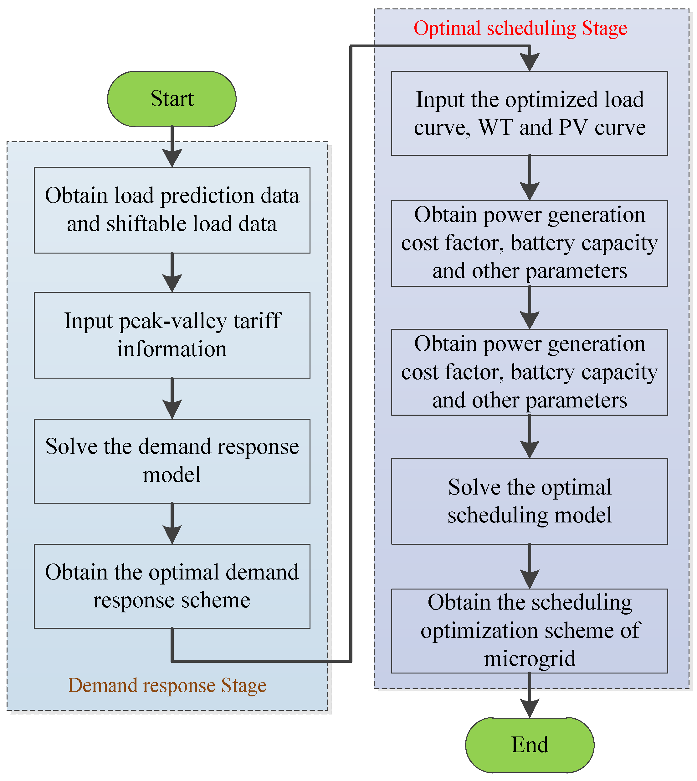
2.3. Demand Response and Optimal Scheduling Model

2.3.1. Demand Response Model

(a)

Demand response strategy

Generally, considering the load attribute, the load in the demand side is divided into rigid load and flexible load. Rigid load cannot be shifted and must be met as it plays an extremely important role, such as hospital electricity and lighting electricity for customers. Flexible load is transferable, and one can decide whether or when to use it depending on the microgrid economy, such as electric vehicles.

The mechanism can be divided into a price-based response mechanism and an e-based demand response mechanism [32].

There are two approaches to demand response. Load adjustments can be made by the electric price and incentives. For instance, price-based demand response is guided by the electricity price, which is different at different periods in one day. Wise users choose to use electricity during special periods of low electricity prices, so as to obtain cost benefits and stabilize the operation. When the power supply of a microgrid is seriously insufficient, some loads are interrupted according to the agreement between the operator and the customer. The customer receives certain financial compensation to achieve the balance of supply and demand, which is called an incentive-based demand response mechanism.

Generally, microgrids are a strong complement to power systems and often operate in grid mode. Therefore, it is considered that the microgrid is in a stable operation state and the power supply can be guaranteed. Under the condition of a stable power supply, emergency interruption of the load is unnecessary. Load transfer can reduce the electricity cost by trimming the peak load and filling the valley load under the constraint of load transfer.

In this study, the daily load in the microgrid is optimized considering the situation that flexible load participates in price-based demand response. It is assumed that the daily load, such as washing machines, disinfection cabinets and electric charging, can be transferred to any time period. Users of electrical appliances can achieve the purpose of reducing the cost of electricity by reasonably arranging the consumption time of electrical equipment. In addition, load optimization improves the stability of microgrid operation.

(b)

Objective function

When the renewable energy output fails to meet the load demand most of the time within a scheduling period, the customer purchases electrical power from the main network. A time-of-use tariff mechanism should be considered in load side demand management to realize the lowest cost of electricity in the adjustable range of load. The expression for the objective function is written in Formula (15).

$$\min F={\displaystyle {\sum }_{i=1}^N[{\sigma }_{buy,i}{P}_{buy,i}-{\sigma }_{sell,i}{P}_{sell,i}]\Delta t}$$

(15)

(c)

Constraint condition.

The demand response constraints include the transfer capacity limitation and the total load balancing constraint. The transfer power of the load should be between the upper limit $L_{in,t}^{\max }$ and the lower limit $L_{in,t}^{\min }$. Similarly, the load power which is rolled out should be between the upper limit $L_{out,t}^{\min }$ and the lower limit $L_{out,t}^{\max }$.

$$L_{in,t}^{\min }\le L_{in,t}\le L_{in,t}^{\max },$$

(16)

$$L_{out,t}^{\min }\le L_{out,t}\le L_{out,t}^{\max },$$

(17)

The total load before and after transferring the load is the same and can be calculated by

$${\displaystyle \sum _{t=1}^T{P}_{load}^{new}(t)=}{\displaystyle \sum _{t=1}^T{P}_{load}(t)},$$

(18)

where $P_{load}^{new}(t)$ and $P_{load}(t)$ are the load in period t after and before transferring the load, respectively.

2.3.2. Optimal Scheduling Model of Microgrid

Further, the optimal scheduling model of a microgrid is presented in this paper. Combined with the demand response model, the optimal load power supply strategy is proposed in detail. The optimal scheduling model is as follows.

(a)

Objective Function

The objective function of the scheduling model is to minimize the comprehensive electricity cost, which is expressed by the following formula:

$$MinC=C_{wt}+C_{pv}+C_{bat}+C_{buy}-C_{sell},$$

(19)

(b)

Constraint condition

• Distributed generation constraint

To protect wind turbines and photovoltaic panels, the output power should be limited:

$$\{\begin{array}{c}0\le P_{wt}\le P_{wt,\max }\\ 0\le P_{pv}\le P_{pv,\max }\end{array},$$

(20)

where P_wt,max and P_pv,max represent the maximum power of wind generation and photovoltaics, respectively.

• Power exchange constraints

In the power system, the total power is balanced, which can be written as

$$P_{wt}+P_{pv}+P_{bat}+P_{buy}-P_{sell}=P_{load},$$

(21)

In addition, the power of the microgrid that interacts with the outside system is limited:

$$\{\begin{array}{c}{P}_{exc,\min }\le P_{buy}\le P_{exc,\max }\\ P_{exc,\min }\le P_{sell}\le P_{exc,\max }\end{array},$$

(22)

where P_exc,max and P_exc,min represent the upper limit and the lower limit of exchange power, respectively.

• Battery constraints.

The restriction of batteries is mainly reflected in the change of the state-of-charge, including the depth and the speed of the battery state.

Firstly, it is necessary to protect the battery from overcharging or over discharging:

$$SO{C}_{\min }\le SO{C}_t\le SO{C}_{\max }$$

(23)

In addition, the charging and discharging speed should not exceed the maximum bearing capacity and the amount of battery discharge within a period of time should be limited to less than 20% of the battery capacity:

$$\left|SO{C}_t-SO{C}_{t-1}\right|E_b\le 0.2E_b,$$

(24)

In addition, the battery life is affected by the use frequency. Hence, the number of uses in a scheduling period needs to meet the constraint:

$${\displaystyle {\sum }_{t=1}^N{N}_t}\le N_{\max },$$

(25)

where N_t is the charging and discharging state at time t, which can be expressed as:

$$N_t=\{\begin{array}{cc}1& (SO{C}_t-SO{C}_{t-1})\ne 0\\ 0& (SO{C}_t-SO{C}_{t-1})=0\end{array},$$

(26)

In addition, the initial state, SOC₀, should be the same as the end state, SOC_T, in a scheduling period.

$$SO{C}_0=SO{C}_{\mathrm{T}}$$

(27)

For the sake of better comprehension, the optimization process of a microgrid is shown in Figure 2.

3. Improved War Strategy Optimization Algorithm

3.1. War Strategy Optimization Algorithm

Ayyarao et al. proposed the WSO algorithm in 2022 by simulating a war strategy [33]. The WSO algorithm is inspired by the attack strategy and the defense strategy of ancient warfare. The optimization problem is solved by updating the soldier’s position on the battlefield. In the search process of the WSO algorithm, a group of feasible solutions is called an army. One of the feasible solutions is regarded as a soldier. The most powerful soldier is called a commander, and the king is the supreme army leader. Soldiers constantly update their positions based on the king’s position and the commander’s position. Meanwhile, the king proposes a reasonable attack strategy according to the war situation. When a soldier is injured in combat or put in a bad position, the soldier position is updated considering new recruit replacement or relocation strategies.

There are four update strategies of the soldier position in the WSO algorithm. However, the algorithm converges slowly and the accuracy is low under the current update strategy. The improved WSO algorithm improves the solving speed and result accuracy by dynamic step sizes. The mathematical description of the improved WSO algorithm is as follows:

• Attack strategy

Soldiers adjust their positions according to the positions of the king and commander, which is the main strategy for soldier position renewal. The mathematical description is:

$$X_i(t+1)=X_i(t)+2\cdot rand\cdot (C-King)+rand\cdot (W_i\cdot King-X_i(t)),$$

(28)

where X_i(t + 1) denotes the new position of the soldier at iteration t + 1, X_i(t) denotes the soldier position at iteration t, C and King are the commander and king, respectively, and W_i is the weight of the king’s position.

• Rank and weight updating

A soldier preferentially chooses better positions in the battlefiled, and the rank of the soldier increases with their combat effectiveness. The mathematical description is:

$$X_i(t+1)=(X_i(t+1))\cdot (F_n\ge F_p)+(X_i(t))\cdot (F_n<F_p),$$

(29)

$$R_i=(R_i+1)\cdot (F_n\ge F_p)+(R_i)\cdot (F_n<F_p),$$

(30)

where F_n is the soldier’s combat effectiveness in the new position, F_p is the soldier’s combat effectiveness in the old position and R_i denotes the rank degree which the i-th soldier takes.

The soldier is ranked according to soldier effectiveness, and the updated weight is represented by Formula (31).

$$W_i=W_i\cdot {(1-R_i/T)}^{\alpha },$$

(31)

where T denotes the iteration number and α is an exponential factor.

• Defense strategy

The soldier measures their distance from the king and protects the king safety in the course of the war. The mathematical description is:

$$X_i(t+1)=X_i(t)+2\cdot rand\cdot (King-X_{rand}(t))+rand\cdot W_i\cdot (C-X_i(t)),$$

(32)

where X_rand(t) is a random position of the soldier at iteration t.

• Replacement/Relocation of weak soldiers

The WSO algorithm uses two methods to renew the positions of weak soldiers. One is to generate new soldiers randomly through Formula (34), while the other is to place weak soldiers in the median position of the entire battlefield through Formula (35).

$$X_w(t+1)=Lb+rand\cdot (Ub-Lb),$$

(33)

$$X_w(t+1)=-(1-randn)\cdot (X_w(t)-median(X))+King,$$

(34)

where X_w(t + 1) are the weak soldiers replaced by iteration t + 1, Ub and Lb are the upper and lower value limits, respectively, randn is a random number evenly distributed between 0 and 1 and median(·) is the median function.

3.2. Improved WSO Algorithm

The rank and weight updating strategy and replacement/relocation of weak soldiers of the WSO algorithm are improved to improve the performance of the algorithm.

• Improved rank and weight updating

In the original algorithm, the exponential factor in the soldier rank is a fixed value. In order to improve the global search ability in the early stage and the convergence ability in the late stage, the exponential factor is set as dynamic.

$$\alpha =2(1-e^{-t/T}),$$

(35)

where t is the iteration number of the algorithm.

• Improved replacement/relocation of weak soldiers

Further, a new replacement/relocation strategy of weak soldiers is innovatively proposed. The strategy breaks down the renewal of weak soldiers into three phases. At the beginning of the algorithm iterations, the update of weak soldiers is completely random, which can enhance the global search ability. In the middle of the iterations, by using the dynamic weighting method, the soldiers gradually tend to the middle of the battlefield, while taking the random search ability into account. In the later iterations, weak soldiers are replaced in the center of the battlefield to achieve better convergence of the algorithm.

$$X_w(t+1)=\{\begin{array}{ll}Lb+rand\cdot (Ub-Lb)\hfill & t\le \frac{1}{3}T\hfill \\ \beta (Lb+rand\cdot (Ub-Lb))+(1-\beta )(-(1-randn)\cdot (X_w(t)-median(X))+King)\hfill & \frac{1}{3}T<t\le \frac{2}{3}T\hfill \\ -(1-randn)\cdot (X_w(t)-median(X))+King\hfill & t>\frac{2}{3}T\hfill \end{array}$$

(36)

$$\beta =e^{1-\frac{3t}{T}},$$

(37)

where β is the temporal weight search factor.

Further, the flow chart of the improved WSO algorithm is shown in Figure 3.

3.3. Parameter Selection

The selection of parameters has a great influence on the performance of the algorithm. In the improved WSO algorithm, the main parameters that affect the performance of the algorithm are the number of soldiers, the number of iterations and the guide factor. Among them, the number of soldiers has the greatest influence on the optimization performance of the algorithm. The more soldiers there are, the larger the space that can be searched in an iteration and the greater the probability of finding the optimal solution. However, as the number of soldiers increases, so does the computational time. The selection of the number of soldiers should ensure the convergence of the algorithm and minimize the computational time. The improved WSO algorithm converges quickly, so long as the number of iterations can ensure algorithm convergence. The guide factor ρ_r is selected based on the objective function. Through the experiments of different test functions, it is concluded that a value in the range of (0–0.5) is the most suitable for unimodal function, and a value in the range of (0.5–1) is the most suitable for multi-modal function [33].

4. Results and Discussion

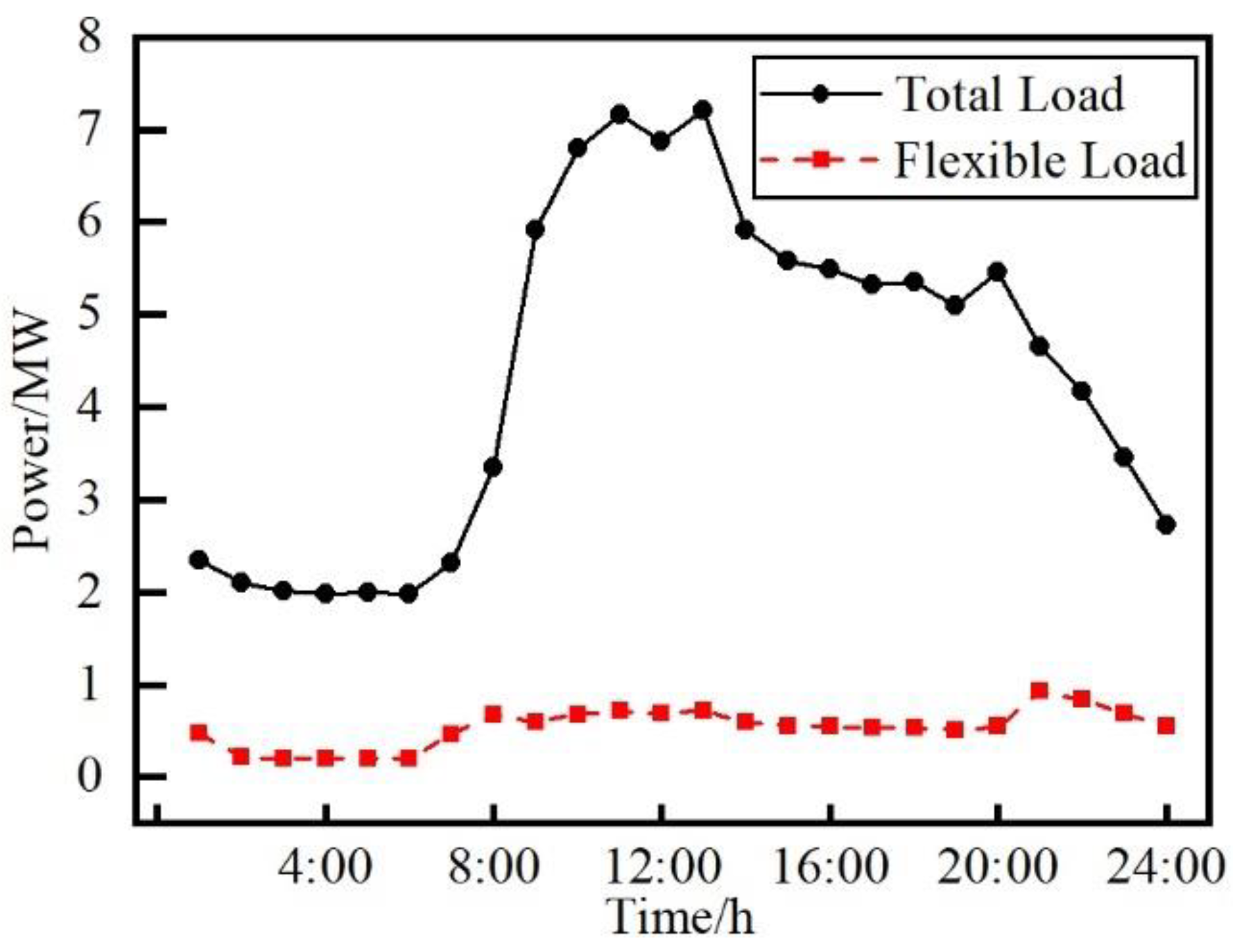
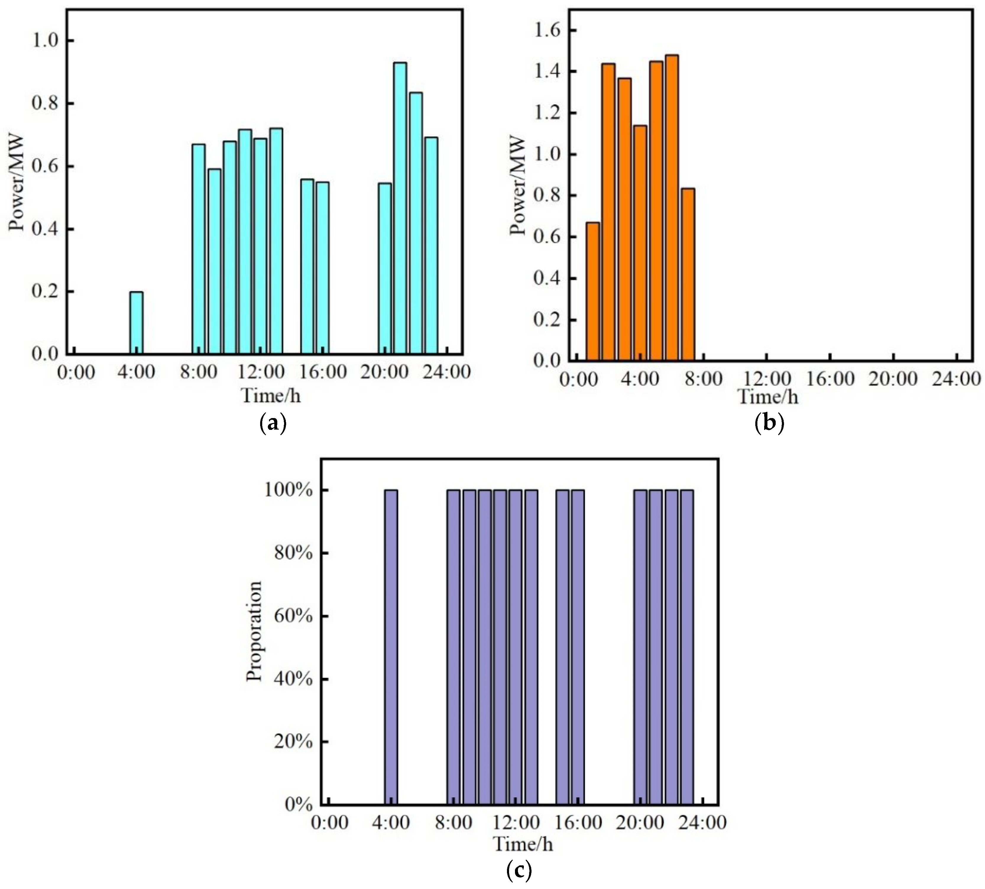
4.1. Demand Response

This paper takes a grid-connected AC microgrid as an example (see Figure 1). The rated powers of the wind generation and photovoltaics are 10 MW and 5 MW, respectively. Figure 4 shows the power curves of wind generation, photovoltaics and load in a scheduling period.

Table 2. Electricity price of each period.

Price Type	Time Period/t	Purchase Price/(CNY/(kW·h))	Selling Price/(CNY/(kW·h))
Valley	1~7, 22~24	0.25	0.22
Normal	8~10, 16~19	0.53	0.42
Peak	11~15, 20~21	0.82	0.65

shows the price list of power exchange between the microgrid and the main network at different periods of a day [34].

The power in the main grid can be purchased when the internal power supply is insufficient. In this case, the interruption of load is unnecessary, and only the shiftable load in the price-based demand response is considered. The power curves of the shiftable load and the total load in a scheduling period are shown in Figure 5.

The PSO algorithm is a mature and robust optimization algorithm that has been verified over many years [35,36,37]. PSO is widely used to solve the optimization problem due to its simplicity and practicality. Hence, PSO is selected to solve the demand response model in a simple scenario in the paper. Taking the lowest power purchase cost as the optimization objective, the load curve is optimized to obtain more revenue. In particular, the population size of the PSO algorithm is 500, and the number of iterations is 300. In addition, the learning factor c₁ = c₂ = 1.49445, and the inertia weight varies dynamically between 0.4 and 0.8 to reduce the solution time. Further, Figure 6 shows the load power with DR and without DR.

Observing Figure 6, the peak value of optimized load is lower than the previous load curve, and the optimized load valley is higher than the load valley before optimization. During the peak period, the price of electricity is high and users transfers load to the valley period with lower electricity which can reduce the electricity cost. The inbound and outbound loads of each period are shown in Figure 7. It is found that the load is transferred out in each period. Load is diverted during the periods from 11 to 15 and from 20 to 21 because the electricity cost is expensive. During the normal period of electricity price, part of the load is transferred out to obtain higher economic benefits. Figure 7b shows the load roll-in in each period, and it can be seen that the load has been shifted into the valley when the price is lower. Figure 7c shows the proportion of transferred load to total transferable load in each period; the full flexible load participates in demand response when it is necessary.

Table 3. Electricity cost before and after demand response.

	Electricity Cost before Demand Response/(CNY)	Electricity Cost after Demand Response/(CNY)
Valley	6277.24	7939.4
Normal	19,778.57	18,458.84
Peak	35,136.06	31,726.01
Total	61,191.87	58,124.25

shows the electricity cost. The total cost for the scheduling period before demand response is CNY 61,191.87, and the cost was reduced to CNY 58,124.25 after demand response. The total cost reduces by CNY 3067.62 per day. The costs during valley, normal and peak hours are calculated. It is found that the electricity cost during the peak period decreases from CNY 35,136.06 to CNY 31,726.01. The total cost in the peak period is reduced by CNY 3410.05, which is the main reason for the reduction in electricity costs. At the same time, the cost during valley hours increased from CNY 6277.24 to CNY 7939.4, which is an increase of CNY 1662.16. Although the electricity cost increases during the valley period, the increase is far less than the decrease during peak hours. In addition, the electricity cost during normal time is also reduced by CNY 1319.73.

4.2. Optimal Scheduling of Microgrid

Further, to verify the positive effect of the microgrid scheduling model and load optimization on reducing the microgrid cost, this paper assumes three different scenarios of microgrid operation. A scheduling period is 24 h, and electrical prices at various times are shown in Table 3. The improved WSO algorithm is adopted.

• Scenario 1: Microgrid operates without batteries

In this scenario, wind and photovoltaic power generation are the priority to supply the load in the microgrid. When the distributed generation supply is sufficient, surplus electricity is used to make profit by selling it to the main network. The load, wind and photovoltaic power in a dispatching cycle are shown in Figure 2. The operation and maintenance coefficients of wind turbines and photovoltaic modules are 0.63 CNY/kW·h and 0.78 CNY/kW·h, respectively. The cost in this scenario is shown in

Table 4. Operating cost of microgrid in scenario 1.

	Cost of Electricity Purchasing	Income from Electricity Sales	Maintenance Cost of Wind Turbine	Maintenance Cost of Photovoltaic Module	Total Cost
Cost/CNY	9583.40	14,828.22	39,562.51	43,475.8	77,793.49

. In the absence of distributed generation, all the power of the grid is supplied by the main network, and the cost of purchasing electricity is CNY 9583.4. The maintenance cost is higher than the unit price of power purchase most of the time. Hence, the operation cost of the microgrid is more expensive when wind and photovoltaic power participate in power scheduling. However, the purchased power decreases from 105.28 MW·h to 17.42 MW·h, indirectly reducing the proportion of thermal power generation, which is the main source of electric power in the main network.

• Scenario 2: Microgrid operates with batteries

In this scenario, wind generated and photovoltaic power can be supplied to the internal load demand, and the remaining energy can be stored in the battery or sold to the main network. In theory, when power generation is sufficient and the price of electricity is low, the priority is to charge the battery. When the power supply within the microgrid is insufficient and the purchase price is high, the battery discharges to reduce the cost of electricity. Further, the optimal scheduling strategy in this scenario is obtained by the improved WSO algorithm. The results are illustrated in Figure 8, Figure 9 and Figure 10.

Figure 8 shows the power curves of load, wind turbines, photovoltaics and the battery in a scheduling period. Figure 9 shows the SOC curve of the battery. In the period from 0:00 a.m. to 7:00 a.m., the photovoltaic output is 0, while the wind power output is enough to meet the load demand. Additionally, there is excess power from renewable energy. At the same time, the electricity prices are lowest, so it makes sense to use the extra energy to charge the battery. The electricity prices are high between 11:00 a.m. and 15:00 p.m. The total power can still meet the load. Additionally, the battery SOC value is high. Hence, the battery discharges and all the excess power is sold to the main network in order to achieve a higher economic benefit. The selling price from 16:00 p.m. to 19:00 p.m. is normal. When there is still a surplus of photovoltaic power, the battery is charged to meet the subsequent high electricity price peak from 20:00 p.m. to 21:00 p.m., and load demand is insufficient. Figure 10 shows the iterative process of the improved WSO algorithm. The curve has converged in the 15th iteration, indicating that the algorithm has strong convergence.

Table 5. Operating cost of microgrid in scenario 2.

	Cost of Electricity Purchasing	Income from Electricity Sales	Maintenance Cost of Wind Turbine	Maintenance Cost of Photovoltaic Module	Maintenance Cost of Battery	Total Cost
Cost/CNY	6211.37	14,596.22	39,562.51	43,475.8	2399.99	77,053.45

shows the composition of electricity consumption cost. Compared to the scenario without batteries, the electricity cost is reduced by CNY 740.04. The cost of purchasing electricity decreased by CNY 3372.03, which is the main reason for the reduction in the electricity cost. Since wind and photovoltaic power are partly used to charge batteries, the sales of electricity are slightly lower. In addition, the charging and discharging of batteries require maintenance costs, resulting in an increase of CNY 2399.99. However, the power purchased power by the microgrid decreased from 17.42 MW·h to 13.02 MW·h due to the addition of a battery.

• Scenario 3: Microgrid operates with batteries and demand response

In addition to batteries, the internal load of the microgrid also is optimized regarding the scheduling strategy under scenario 3. The scheduling strategy has two steps. The first step is the load optimization based on the demand response, as indicated in Figure 4. The second step is the optimal allocation of the electricity power on the basis of the load optimization. Additionally, the improved WSO algorithm is used in the second step. The results are shown in Figure 11, Figure 12 and Figure 13.

Observing Figure 11 and Figure 12, when the load participates in demand response, the electricity consumption increases obviously during valley periods from 0:00 to 7:00. During this time, the power from wind turbines is able to meet the load. However, it is not enough at some particular points. Hence, the load is supported by purchasing electricity from main network at these special points. It is economical to purchase power from the main network during this period to fill up the battery because the electricity prices during this period are the lowest in a day. Similar to scenario 2, the battery discharges from 14:00 to 15:00 and 19:00 to 21:00 due to the high prices. Meanwhile, the battery is fully charged from 16:00 to 17:00 when the electricity price is relatively low. Figure 13 shows the iterative process of the algorithm in scenario 3. The WSO convergence rate is still very fast, and it has converged in the seventh iteration.

Table 6. Operating cost of microgrid in scenario 3.

	Cost of Electricity Purchasing	Income from Electricity Sales	Maintenance Cost of Wind Turbine	Maintenance Cost of Photovoltaic Module	Maintenance Cost of Battery	Total Cost
Cost/CNY	5180.86	16,181.11	39,562.5	43,475.8	2399.99	74,438.04

shows the details of electricity cost in this scenario. Compared with the cost under scenario 1 and scenario 2, the purchasing cost decreased significantly by CNY 1106.44 under scenario 3. In fact, the total load has not decreased. On the one hand, the electricity purchased from the main network is lower due to load transfer. It is worth noting that the reduction is small, only about 0.079 MW·h. The load is transferred to periods with a low electricity price. Hence, the reduction in power purchases is obvious. As the load is transferred to the period of low electricity prices, more electricity can be sold to the main network with a high electricity price. Hence, the income from power sales increases by CNY 1457.18. The maintenance cost of batteries does not change because the SOC value of the battery in a scheduling period is constant.

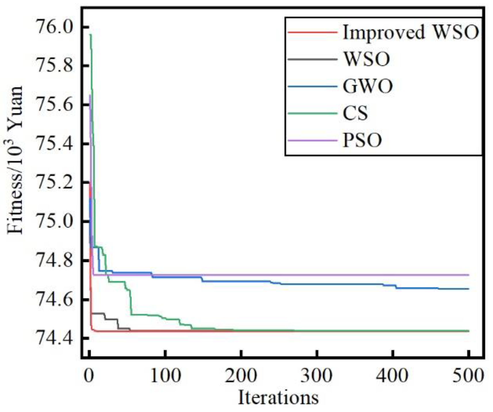
4.3. Algorithm Comparison

To verify the superiority of the improved WSO algorithm, different algorithms and the WSO algorithm were selected to calculate the proposed model in scenario 3 [37,38,39]. The parameter settings of each algorithm are shown in

Table 7. Algorithm parameters.

Algorithm	Parameter	Value
PSO	Pop Size	p = 1000
	Number of iterations	G = 500
	Learning factor	c1 = c2 = 1.49445
	Inertia weight	wmax = 0.8, wmin = 0.4
	Flight speed	Vmax = 1, Vmin = −1
CS	Number of nests	N = 1000
	Number of iterations	G = 500
	Discovery probability	Pa = 0.25
	Step size scaling factor	α = 1
GWO	Pop Size	p = 1000
	Number of iterations	G = 500
	Convergence factor	decreases linearly from 2 to 0
WSO	Number of soldiers	p = 1000
	Number of iterations	G = 500
	Guide factor	ρr = 0.8
Improved WSO	Number of soldiers	p = 1000
	Number of iterations	G = 500
	Guide factor	ρr = 0.8

. Different background colors in the table indicate different algorithm. Electricity costs and computation times are listed in

Table 8. Algorithm comparison.

Algorithm	Cost/CNY	Iterations	Computation Time/s
PSO	74,726.13	500	7.344387
CS	74,438.17	500	15.42264
GWO	74,654.15	500	4.549247
WSO	74,438.08	500	1.952064
Improved WSO	74,438.04	500	1.895227

after 500 iterations. Compared with the other four algorithms, the electricity cost obtained by improved WSO is lowest. At the same time, the improved WSO algorithm takes the shortest computation time with the same iteration number as the other algorithms. The iterative process of the five algorithms is shown in Figure 14. It shows that the improved WSO algorithm has the fastest convergence speed and the best solution among the five algorithms.

Table 9. Cost composition analysis.

	PSO	CS	GWO	WSO	Improved WSO
Wind	39,562.5	39,562.5	39,562.5	39,562.5	39,562.5
Photovoltaic	43,475.8	43,475.8	43,475.8	43,475.8	43,475.8
Battery	2879.99	2400.26	2160.165	2400	2399.99
Purchase	6028.88	5181.31	5637.17	5180.88	5180.86
Sell	17,221.04	16,181.69	16,181.5	16,181.11	16,181.11
Total cost	74,726.13	74,438.17	74,654.15	74,438.08	74,438.04
Computational time/s	7.344387	15.42264	4.549247	1.952064	1.895227

shows the microgrid electricity cost using the five algorithms. As wind generated and photovoltaic power are constant, the maintenance cost of wind turbines and photovoltaics obtained by the four algorithms is same, while the maintenance cost of the battery is slightly different because the charging and discharging strategies obtained by the algorithms are different. The results obtained by the CS algorithm, the WSO algorithm and the improved WSO algorithm are very similar, but the computation times of the CS algorithm and the WSO algorithm are longer than that of the improved WSO algorithm. In addition, the convergence rate of the improved WSO algorithm is faster than the CS algorithm. The result shows that the improved WSO algorithm has both a powerful optimization ability and computational efficiency.

5. Conclusions

This paper proposed an economic scheduling model for microgrids under the mechanism of a peak–valley tariff. In contrast to previous scheduling strategies, the demand response of the microgrid is utilized to optimize the load curve and improve the economy of microgrid operation. Furthermore, a scheduling model is established by the interaction of distributed generation, battery and load. Three typical scenarios are selected considering the battery and demand response. In addition, the improved WSO algorithm is used to solve the optimal scheduling model in three microgrid scenarios. The WSO algorithm is considerably improved by introducing a dynamic and time-weighted search factor to modify the replacement strategy of weak soldiers in the algorithm.

The results show the load translation is conducive to obtaining more revenue and reducing the power supply pressure in the peak period. Meanwhile, the microgrid can obtain higher economic benefits through a reasonable and valid plan of battery use and power supply. In addition, the comparison results also verify the superior performance of the improved WSO algorithm.

References

1. Zhang, J.; Chen, Z. The Impact of AMI on the Future Power System. Autom. Electr. Power Syst. 2010, 34, 10–14+23. [Google Scholar]
2. Gang, W.Q.; Cun, Y.M.; Zhao, Z.Y.; Jie, Z.Y.; Hong, L.J.; Tao, G. Review on Evaluation Methods of Combined Heating, Power and Biogas System Coupled With Renewable Energy. Power Syst. Technol. 2021, 45, 937–950. [Google Scholar]
3. Strategy for revolution in energy production and consumption (2016–2030). Electr. Appl. Ind. 2017, 5, 39–47.
4. Caineng, Z.; Dongbo, H.; Chengye, J.; Bo, X.; Qun, Z.; Songqi, P. Connotation and pathway of world energy transition and its significance for carbon neutral. Acta Pet. Sin. 2021, 42, 233–247. [Google Scholar]
5. Alasseri, R.; Tripathi, A.; Rao, T.J.; Sreekanth, K.J. A review on implementation strategies for demand side management (DSM) in Kuwait through incentive-based demand response programs. Renew. Sustain. Energy Rev. 2017, 77, 617–635. [Google Scholar] [CrossRef]
6. Vardakas, J.S.; Zorba, N.; Verikoukis, C.V. A survey on demand response programs in smart grids: Pricing methods and optimization algorithms. IEEE Commun. Surv. Tutor. 2014, 17, 152–178. [Google Scholar] [CrossRef]
7. Li, Y.; Yang, Z.; Li, G.; Mu, Y.; Zhao, D.; Chen, C.; Shen, B. Optimal scheduling of isolated microgrid with an electric vehicle battery swapping station in multi-stakeholder scenarios: A bi-level programming approach via real-time pricing. Appl. Energy 2018, 232, 54–68. [Google Scholar] [CrossRef] [Green Version]
8. Wang, J.; Zhong, H.; Lai, X.; Xia, Q.; Shu, C.; Kang, C. Distributed real-time demand response based on Lagrangian multiplier optimal selection approach. Appl. Energy 2017, 190, 949–959. [Google Scholar] [CrossRef]
9. Navin, N.K.; Sharma, R. A fuzzy reinforcement learning approach to thermal unit commitment problem. Neural Comput. Appl. 2019, 31, 737–750. [Google Scholar] [CrossRef]
10. Lu, R.; Hong, S.H. Incentive-based demand response for smart grid with reinforcement learning and deep neural network. Appl. Energy 2019, 236, 937–949. [Google Scholar] [CrossRef]
11. Wei, C.; Shen, Z.; Xiao, D.; Wang, L.; Bai, X.; Chen, H. An optimal scheduling in interconnected microgrids based on RO and Nash strategy for peer-to-peer trading bargaining. Appl. Energy 2021, 295, 117024. [Google Scholar] [CrossRef]
12. Shuai, H.; Fang, J.; Ai, X.; Tang, Y.; Wen, J.; He, H. Stochastic Optimization of Economic Dispatch for Microgrid Based on Approximate Dynamic Programming. IEEE Trans. Smart Grid 2019, 10, 2440–2452. [Google Scholar] [CrossRef] [Green Version]
13. Gong, Y.; Yang, X.; Xu, J.; Chen, C.; Zhao, T.; Liu, S.; Lin, Z.; Yang, L.; Qian, H.; Ke, C. Optimal operation of integrated energy system considering virtual heating energy storage. Energy Rep. 2021, 7, 419–425. [Google Scholar] [CrossRef]
14. Wang, Y. Coordinated Heat and Power Scheduling of Micro-Energy Grid Considering Heat Balance Model of Building and Indoor Comfort Demand. Master’s Thesis, Tianjin University, Tianjin, China, 2018. [Google Scholar]
15. Khalili, T.; Nojavan, S.; Zare, K. Optimal performance of microgrid in the presence of demand response exchange: A stochastic mufti-objective model. Comput. Electr. Eng. 2019, 74, 429–450. [Google Scholar] [CrossRef]
16. Yang, H.; Shi, B.; Huang, W.; Ding, Y.; Wang, J.; Yu, W.; Zhu, Z. Day-Ahead Optimized Operation of Micro Energy Grid Considering Integrated Demand Response. Electr. Power Constr. 2021, 42, 75–82. [Google Scholar]
17. Zhang, Y.; Lin, X.; Xu, Z.; Chen, Z. Dispatching Method of Micro-energy Grid Based on Light Robust Optimization. Autom. Electr. Power Syst. 2018, 42, 75–82. [Google Scholar]
18. Ma, T.; Wu, J.; Hao, L. Energy Flow Modeling and Optimal Operation Analysis of Micro Energy Grid Based on Energy Hub. Power Syst. Technol. 2018, 42, 75–82. [Google Scholar] [CrossRef]
19. Chen, F.; Deng, H.; Shao, Z. Distributed robust synergistic scheduling of electricity, natural gas; heating and cooling systems via alternating direction method of multipliers. Int. J. Energy Res. 2021, 45, 8456–8473. [Google Scholar] [CrossRef]
20. Wang, J.; Shi, J.; Wen, F.; Li, J.; Zhang, L. Optimal Operation of CHP Microgrid with Concentrating Solar Power Plants Considering Demand Response. Autom. Electr. Power Syst. 2019, 43, 176–185. [Google Scholar]
21. Zhang, H.; Cheng, Z.; Jia, R.; Zhou, C.; Li, M. Economic Optimization of Electric-gas Integrated Energy System Considering Dynamic Characteristics of Natural Gas. Power Syst. Technol. 2021, 45, 1304–1311. [Google Scholar]
22. Chedid, R.; Sawwas, A.; Fares, D. Optimal design of a university campus micro-grid operating under unreliable grid considering PV and battery storage. Energy 2020, 200, 117510. [Google Scholar] [CrossRef]
23. Gabbar, H.A.; Abdussami, M.R.; Adham, M.I. Optimal planning of nuclear-renewable micro-hybrid energy system by particle swarm optimization. IEEE Access 2020, 8, 181049–181073. [Google Scholar] [CrossRef]
24. Xingshen, L.I.; Jing, Z.; Yu, H.E.; Ying, Z.; Ying, L.; Kaifeng, Y. Multi-objective Optimization Dispatching of Microgrid Based on Improved Particle Swarm Algorithm. Electr. Power Sci. Eng. 2021, 37, 1. [Google Scholar]
25. Zhang, L.; Guo, H.; Yao, L. Research on Microgrid Optimization Based on Improved Bat Algorithm. Power Syst. Clean Energy 2021, 37, 122–126. [Google Scholar]
26. Wang, P.-Y.; Gao, M.-H.; Li, G.-L.; Wang, Y.-T. Multiple Objective Optimization of Microgrid Based on Distributed Neural Dynamics Algorithm. Sci. Technol. Eng. 2021, 21, 4063–4070. [Google Scholar]
27. Liu, Y.; Zhang, H. Optimization of Units’ Restoration Sequence Based on Minimizing Risk of Electrical Energy Loss. Autom. Electr. Power Syst. 2015, 39, 30–36+53. [Google Scholar]
28. Kim, H.-J.; Kim, M.-K.; Lee, J.-W. A two-stage stochastic p-robust optimal energy trading management in microgrid operation considering uncertainty with hybrid demand response. Int. J. Electr. Power Energy Syst. 2021, 124, 106422. [Google Scholar] [CrossRef]
29. Imchen, S.; Das, D.K. Scheduling of distributed generators in an isolated microgrid using opposition based Kho-Kho optimization technique. Expert Syst. Appl. 2023, 229, 0957–4174. [Google Scholar] [CrossRef]
30. Basak, S.; Bhattacharyya, B. Optimal scheduling in demand-side management based grid-connected microgrid system by hybrid optimization approach considering diverse wind profiles. ISA Trans. 2023, 19–578. [Google Scholar] [CrossRef]
31. Premadasa, P.N.D.; Silva, C.M.M.R.S.; Chandima, D.P.; Karunadasa, J.P. A multi-objective optimization model for sizing an off-grid hybrid energy microgrid with optimal dispatching of a diesel generator. J. Energy Storage 2023, 68, 107621. [Google Scholar] [CrossRef]
32. Haowu, C.; Shenghong, L.; Jianquan, Z. Bi-level Optimization of Microgrid Economic Dispatch Considering Demand-side Response. Power Syst. Auromation 2023, 45, 79–84. [Google Scholar]
33. Ayyarao, T.S.; Ramakrishna, N.S.S.; Elavarasan, R.M.; Polumahanthi, N.; Rambabu, M.; Saini, G.; Khan, B.; Alatas, B. War Strategy Optimization Algorithm: A New Effective Metaheuristic Algorithm for Global Optimization. IEEE Access 2022, 10, 25073–25105. [Google Scholar] [CrossRef]
34. Manbachi, M.; Ordonez, M. Intelligent Agent-Based Energy Management System for Islanded AC–DC Microgrids. IEEE Trans. Ind. Inform. 2020, 16, 4603–4614. [Google Scholar] [CrossRef]
35. Yavuz, A.; Celik, N.; Chen, C.-H. A Sequential Sampling-based Particle Swarm Optimization to Control Droop Coefficients of Distributed Generation Units in Microgrid Clusters. Electr. Power Syst. Res. 2023, 216, 109074. [Google Scholar] [CrossRef]
36. Rodriguez, M.; Arcos, D.; Martinez, W. Fuzzy logic-based energy management for isolated microgrid using meta-heuristic optimization algorithms. Appl. Energy 2023, 335, 120771. [Google Scholar] [CrossRef]
37. Wu, Z.; Luo, Y.; Hu, S. Optimization of jamming formation of USV offboard active decoy clusters based on an improved PSO algorithm. Def. Technol. 2023, 2214–9147. [Google Scholar] [CrossRef]
38. Singh, P.; Anwer, N.J.S.; Lather, J.S. Energy management and control for direct current microgrid with composite energy storage system using combined cuckoo search algorithm and neural network. J. Energy Storage 2022, 55, 105689. [Google Scholar] [CrossRef]
39. Naserbegi, A.; Aghaie, M.; Zolfaghari, A. Implementation of Grey Wolf Optimization (GWO) algorithm to multi-objective loading pattern optimization of a PWR reactor. Ann. Nucl. Energy 2020, 148, 107703. [Google Scholar] [CrossRef]
Figure 1. Microgrid structure.
Electronics 12 02721 g001
Figure 2. Flow chart of microgrid optimization.
Electronics 12 02721 g002
Figure 3. Flow chat of WSO.
Electronics 12 02721 g003
Figure 4. Power of load, wind generation and photovoltaic generation.
Electronics 12 02721 g004
Figure 5. Shiftable load and total load for each period.
Electronics 12 02721 g005
Figure 6. Load optimization result.
Electronics 12 02721 g006
Figure 7. Load transfer in each period: (a) the load transferred out; (b) the load transferred in; (c) transfer load ratio.
Electronics 12 02721 g007
Figure 8. Power supply components in scenario 2.
Electronics 12 02721 g008
Figure 9. SOC curve of battery in scenario 2.
Electronics 12 02721 g009
Figure 10. Curve of fitness value with the number of iterations in scenario 2.
Electronics 12 02721 g010
Figure 11. Power supply components in scenario 3.
Electronics 12 02721 g011
Figure 12. SOC curve of battery in scenario 3.
Electronics 12 02721 g012
Figure 13. Curve of fitness value with the number of iterations in scenario 3.
Electronics 12 02721 g013
Figure 14. Algorithm comparison.
Electronics 12 02721 g014