SL-Swin: A Transformer-Based Deep Learning Approach for Macro- and Micro-Expression Spotting on Small-Size Expression Datasets

Abstract

In recent years, the analysis of macro- and micro-expression has drawn the attention of researchers. These expressions provide visual cues to an individual’s emotions, which can be used in a broad range of potential applications such as lie detection and policing. In this paper, we address the challenge of spotting facial macro- and micro-expression from videos and present compelling results by using a deep learning approach to analyze the optical flow features. Unlike other deep learning approaches that are mainly based on Convolutional Neural Networks (CNNs), we propose a Transformer-based deep learning approach that predicts a score indicating the probability of a frame being within an expression interval. In contrast to other Transformer-based models that achieve high performance by being pre-trained on large datasets, our deep learning model, called SL-Swin, which incorporates Shifted Patch Tokenization and Locality Self-Attention into the backbone Swin Transformer network, effectively spots macro- and micro-expressions by being trained from scratch on small-size expression datasets. Our evaluation outcomes surpass the MEGC 2022 spotting baseline result, obtaining an overall F1-score of 0.1366. Additionally, our approach performs well on the MEGC 2021 spotting task, with an overall F1-score of 0.1824 and 0.1357 on the CAS(ME)${}^2$ and SAMM Long Videos, respectively. The code is publicly available on GitHub.

1. Introduction

Facial expressions, usually conveyed and perceived by an individual through movements of facial muscles, are a form of non-verbal communication that provides visual cues to an individual’s emotional state. Macro-Expressions (MaEs) and Micro-Expressions (MEs) are two categories of facial expressions that vary according to their intensity and duration. MaEs, which occur at higher intensities, involve facial movements that cover a large facial area. They usually last from 0.5 s to 4.0 s, and can be easily identified from a single frame in a MaE video sequence. Conversely, Micro-Expressions (MEs) are subtle and have a shorter duration (usually within 0.5 s [1]), making them more challenging to spot than MaEs.

Generally, facial expressions pass through three distinct phases: onset, apex, and offset. As described in [2], the onset phase marks the beginning of the facial muscle contraction (the first frame at which an expression starts), the apex phase represents the facial action at its peak intensity, and the offset phase indicates the return of the facial muscles to a neutral state (the last frame at which an expression ends). The concept of expression analysis comprises two aspects, namely, spotting and recognition [3]. The spotting task is designated to identify whether a given video contains expressions and to locate the expression intervals from the onset to the offset phases if these can be found in the video. The task of expression recognition involves categorizing expressions into predetermined emotion types, such as surprise, sadness, happiness, anger, etc. In this paper, our approach is to address the spotting task. It is important to spot expressions, as expressions can provide clues for potential applications such as lie detection and policing, as well as because spotting can reduce the labor required to collect expression data [4].

The existing macro- and micro-expression spotting approaches can be roughly divided into traditional approaches and deep learning approaches [5]. Traditional expression spotting approaches use manually crafted features to determine whether or not a frame is an expression frame. The method proposed by Davison et al. [6] involves splitting faces into blocks and calculating the HOG for each frame. Afterwards, this method spots micro-expressions using the Chi-Squared distance to calculate the dissimilarity between frames at a set interval. Duque et al. [7] proposed the Riesz pyramid-based method. Wang et al. [4] characterized the magnitude of maximal difference in the main direction of optical flow using their proposed Main Directional Maximal Differences (MDMD) method. Zhang et al. [8] and the baseline MEGC2020 [9] method both used optical flow-based approaches to spot expressions, proving that it is possible to extract facial expression movements by describing facial movements using optical flow features, especially the extraction of micro-expressions, which are more subtle and shorter in duration [10].

Traditional approaches limit the representation capability of features when they are extracted manually. While these approaches perform well in spotting MaEs, their ability to spot MEs when the features present extremely weak differences is much less compelling. With the development of deep learning, researchers have applied deep learning methods to overcome the limitations of traditional approaches. Zhang et al. [11] first introduced deep learning to micro-expression spotting, utilizing a Convolutional Neural Network (CNN) to detect the apex frame and then merging nearby detected samples using their proposed feature engineering method. Pan et al. [12] proposed selecting the usefulness of regions of interest (ROI) and adopted a Bilinear Convolutional Neural Network (BCNN) for expression spotting. Building on the baseline of MEGC2021 [13] and MEGC2022 [14], Yap et al. [15] applied frame skipping and contrast enhancement based on a 3D-CNN network. Furthermore, Verburg et al. [16] proposed an approach in which the Histogram of Oriented Optical Flow features of a sliding window were extracted as input features for an RNN composed of LSTM units; this was the first utilization of a Recurrent Neural Network (RNN) for expression spotting.

Though Convolutional Neural Networks (CNNs) have dominated in Computer Vision (CV) research, including expression spotting and recognition, the prevalent architecture today in Natural Language Processing (NLP) instead relies on self-attention-based architectures, particularly Transformers [17]. Inspired by the successes of Transformers in NLP, Dosovitski et al. [18] applied a standard Transformer directly to images, attaining excellent results on image recognition benchmarks such as ImageNet [19]. Considering the compelling performance Transformers have achieved on NLP and CV tasks, researchers have tried combining CNNs with Transformers for expression spotting. Pan et al. [20] proposed the Spatio-Temporal Convolutional Emotional Attention Network (STCEAN), which extracts spatial features through a convolution neural network and employs a self-attention model to analyze the weights of different emotions in the temporal dimension for spotting. The BERT network [21], which is a stack of Transformer encoders based on a bidirectional self-attention mechanism, thrives in Natural Language Processing (NLP) tasks. Coupled with 3D-CNN in the approach proposed by Zhou et al. [22], BERT has shown outstanding behavior in extracting spatio-temporal features. Guo et al. [23] proposed a convolutional transformer network that uses a multi-scale local Transformer module to attain the correlation between frames based on the visual features extracted by a 3D convolutional subnetwork. Compared to expression recognition, however, the use of Transformers in expression spotting is limited.

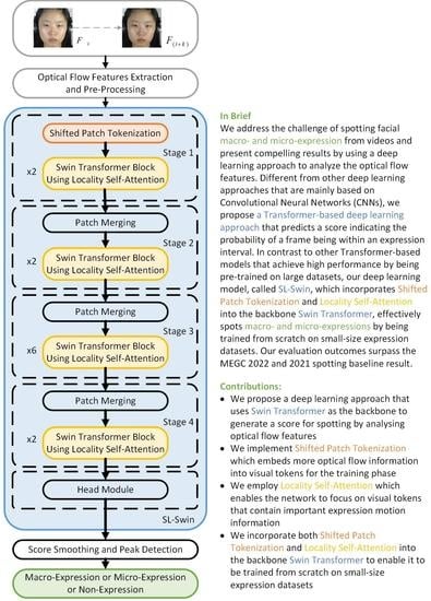
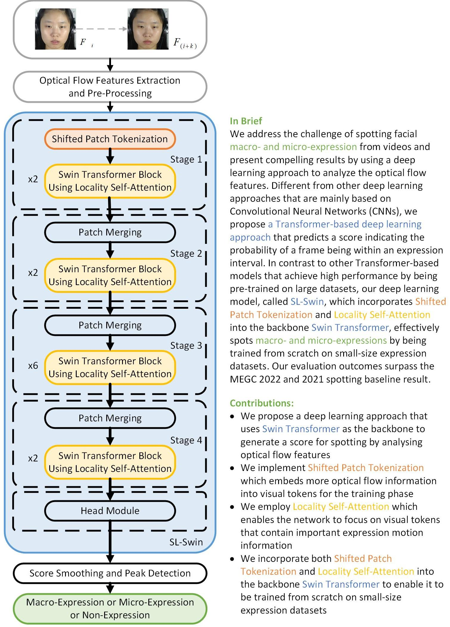
As demonstrated by Liong et al. [24] and Liong et al. [25], the spotting task can be fashioned as a regression problem that predicts the probability of a frame being within a macro- or micro-expression interval. Deep learning models can be trained to discover the expression motion information hidden in the optical flow features. Inspired by the above work, we propose a Transformer-based deep learning approach for spotting macro- and micro-expression by analyzing the optical flow features extracted from videos. Our deep learning model, called SL-Swin, applies Shifted Patch Tokenization (SPT) [26] and Locality Self-Attention (LSA) [26] to the backbone Swin Transformer [27], achieving compelling results after being trained from scratch on small-size expression datasets. In addition, we facilitate the feature learning process by applying the pseudo-labeling technique [25] in the training phase, and predict the apex frame in each video by employing the peak detection technique [28] after the smoothing process. The contributions of this paper are listed below:

• We propose a deep learning approach that uses Swin Transformer as the backbone to generate a score for spotting expressions by analyzing optical flow features.
• We implement SPT, which provides a wider receptive field than standard tokenization, to embed more spatial optical flow information into visual tokens for the training phase.
• We employ LSA, which impels the attention to work locally by forcing each token to concentrate more on tokens with large relation to itself, to enable the network to pay more attention to visual tokens that contain important expression motion information.
• We incorporate both SPT and LSA into the Swin Transformer backbone to enable training from scratch on small-size expression datasets; our study demonstrates the effectiveness of the Transformer-based deep learning approach by outperforming the MEGC 2022 spotting baseline approach and achieving comparable outcomes on the MEGC 2021 spotting task.

2. Materials and Methods

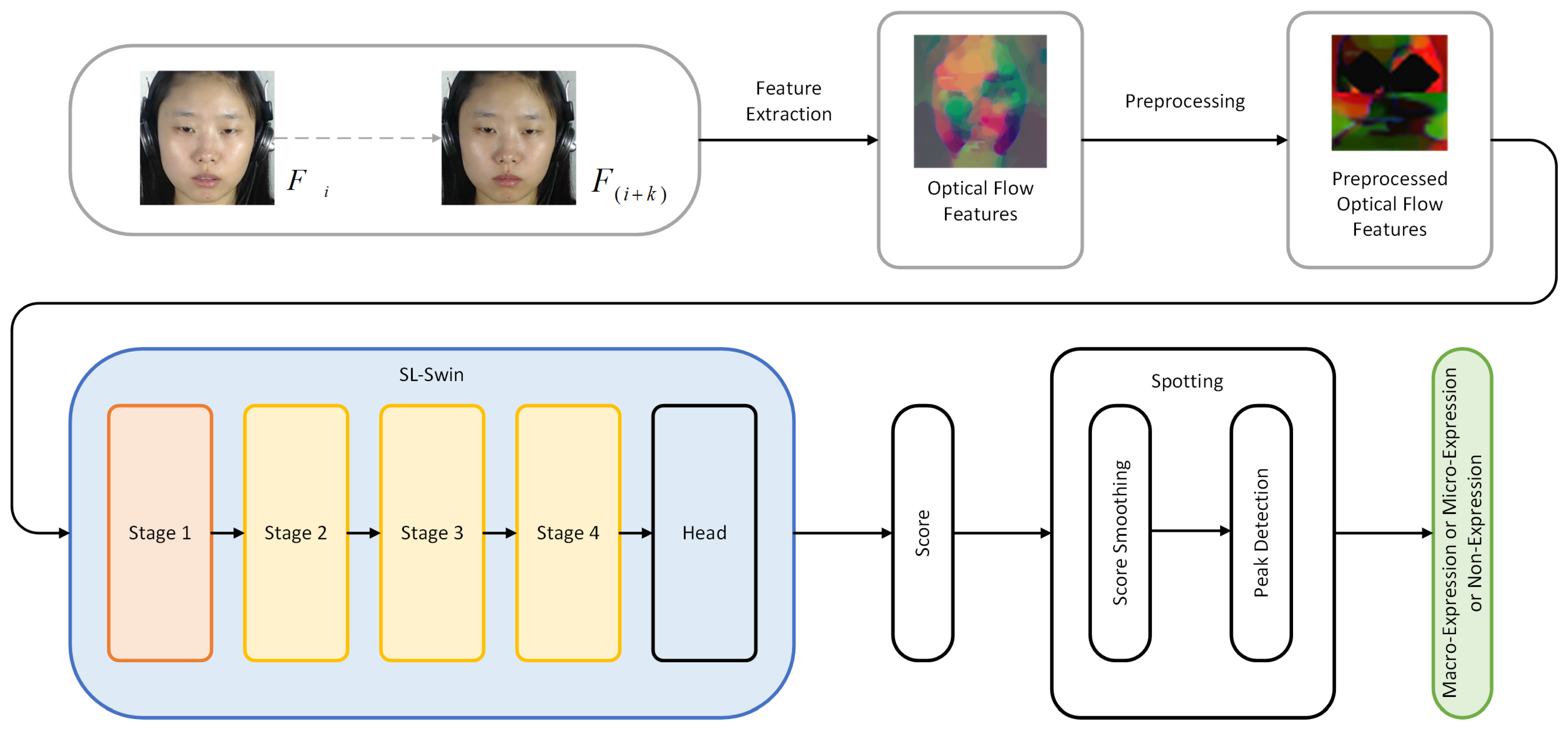
In this paper, we spot MaE and ME in a given video separately. We use the SL-Swin model to generate an expression score to predict the possibility of a frame within the interval of an expression. The proposed approach is illustrated in Figure 1. Five phases of our approach are outlined: initial feature extraction of optical flow features, preprocessing, optical flow features learning using SL-Swin, pseudo-labeling, and expression spotting.

2.1. Feature Extraction

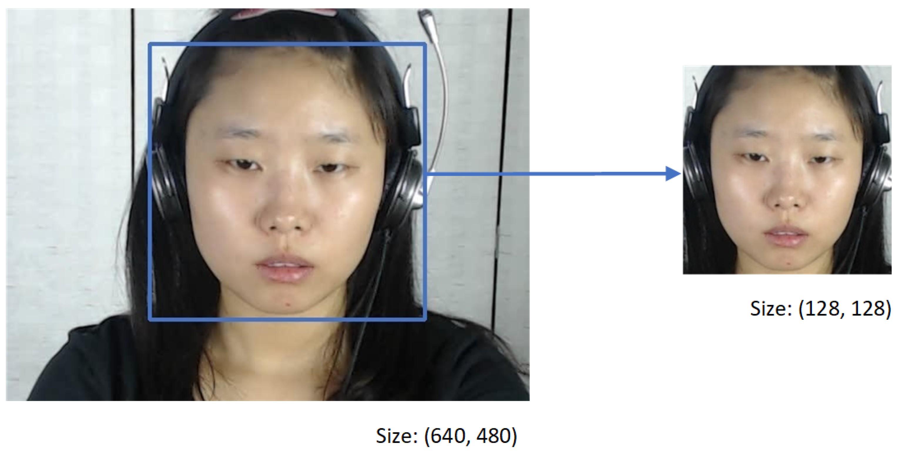
We used optical flow features, which carry substantial spatio-temporal motion information [24,25], as the input for the deep learning model. To begin with, we cropped the facial region in each frame and resized it to $128\times 128$ pixels for resolution normalization. Cropping was carried out on every frame of every raw video using OpenCV’s DNN Face Detector, which is based on a Single-Shot-Multibox detector and uses the ResNet-10 Architecture as its backbone. An example of the cropping process is illustrated in Appendix B.

Next, the current frame $F_i$ and frame $F_{(i+k)}$ (the k-th frame from the current frame $F_i$) were used to compute the optical flow features, where k is half of the average length of an expression interval. Because the TV-L1 optical flow estimation method is the most robust among all optical flow estimation methods tested in [29], we used it to compute the horizontal component u and vertical component v that consist of the first and second channel of the model input features. In addition, we used them to compute the optical strain $ϵ$, which catches subtle facial deformations from optical flow components [30]:

$$ϵ=\left[\begin{array}{cc}{ϵ}_{xx}=\frac{\delta u}{\delta x}& {ϵ}_{xy}=\frac{1}{2}\left(\frac{\delta u}{\delta y}+\frac{\delta v}{\delta x}\right)\\ {ϵ}_{yx}=\frac{1}{2}\left(\frac{\delta v}{\delta x}+\frac{\delta u}{\delta y}\right)& {ϵ}_{yy}=\frac{\delta v}{\delta y}\end{array}\right]$$

(1)

where ${ϵ}_{xy}$ and ${ϵ}_{yx}$ are shear strain components and ${ϵ}_{xx}$ and ${ϵ}_{yy}$ are normal strain components. The third channel of the features that is fed into the model is the optical strain magnitude $\left|ϵ\right|$, which can be computed as

$$\left|ϵ\right|=\sqrt{{ϵ}_{xx}^2+{ϵ}_{yy}^2+{ϵ}_{xy}^2+{ϵ}_{yx}^2}$$

(2)

To sum up, the input data for preprocessing ahead of the model training phase involved the concatenation of the three components $(u,v,|ϵ\left|\right)$ with respective shapes $(128,128,3)$.

2.2. Preprocessing

Prior to model learning, we preprocessed the extracted optical flow features to ensure data consistency and remove noise. Motivated by the work of [8], we subtracted the mean feature of the nose region to eliminate the head motion of each frame.

Because eye blinking significantly disturbs the optical flow features [31], a black polygon-shaped mask was applied to the left and right eye regions, with an additional margin of 15 pixels along the height and width. Next, on the basis that the eyebrows and mouth contain significant movements [31], we used three rectangular boxes of 12 pixels each as the additional margin to enclose three regions as ROIs: ROI 1, spanning the region of the left eye and left eyebrow, was acquired and resized to $21\times 21$; ROI 2, the region of the right eye and right eyebrow, was acquired and resized in the same way; finally, ROI 3, originating from the region of the mouth, was acquired and resized to $21\times 42$.

Eventually, the final preprocessed optical flow features $(u,v,|ϵ\left|\right)$ with respective shapes $(42,42,3)$ used in the training phase were acquired through the following steps. First, the resized ROI 1 and ROI 2 were horizontally stacked to form an upper portion with a size of $21\times 42$. The resized ROI 3, composing the lower portion, was then vertically stacked under the upper portion.

2.3. SL-Swin

To spot expressions by training from scratch on small-size expression datasets, we propose SL-Swin with three further considerations: (1) the backbone of the network is Swin Transformer [27], which is able to effectively consider the local and global features of the expression optical flow features; (2) Shifted Patch Tokenization (SPT) [26] and Locality Self-Attention (LSA) [26] are applied to the backbone, allowing the network to be trained from scratch even on small-size expression datasets; (3) a head module is added to predict a score indicating the probability of a frame being within an expression interval.

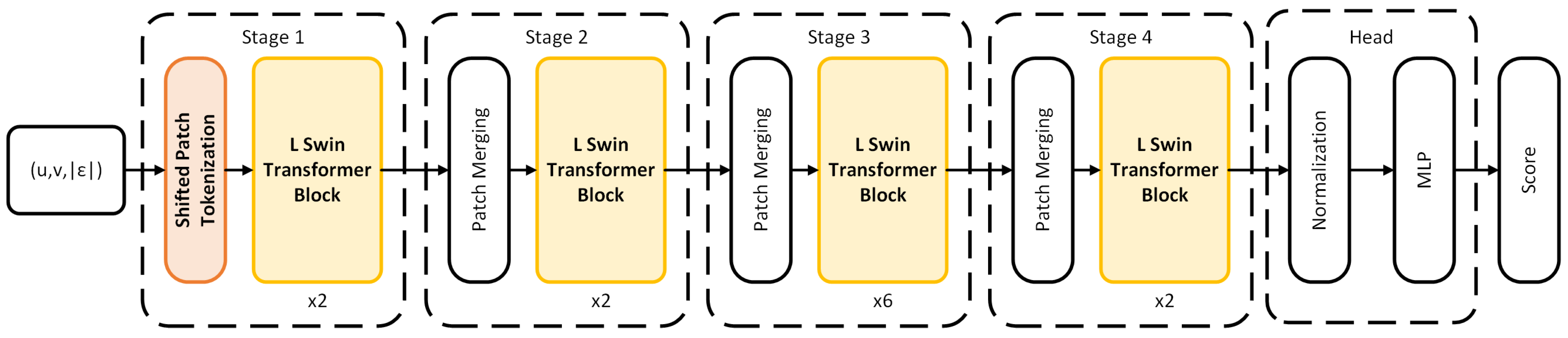
Figure 2 illustrates an overview of the SL-Swin-T model, which is based on the tiny version of the Swin Transformer (Swin-T). Here, SL means that both SPT and LSA are applied to the model. To begin, in “Stage 1” the SPT module splits the input optical flow features into non-overlapping patches which are treated as “visual tokens”. In our approach, the patch size p is 6 and the output is projected to dimension C by a linear embedding layer in SPT. Next, the tokens pass through several Transformer blocks with LSA (L Swin Transformer blocks), which maintain the resolution of the tokens at $(\frac{H}{6}\times \frac{W}{6})$, where H and W are respectively the width and weight of the preprocessed optical flow features input to the model.

The number of tokens is decreased using patch merging layers in the following stages as the network becomes deeper, as the backbone Swin Transformer is designed to build hierarchical feature maps. The patch merging layer decreases the number of tokens by a multiple of $2\times 2=4$ ($2\times$ downsampling of resolution) by concatenating the tokens of each group of $2\times 2$ adjacent patches. Then, a linear layer within the patch merging layer is applied to project the downsampled $4C$-dimensional concatenated features to the $4C$-dimensional output. Afterwards, feature transformation is conducted by several L Swin Transformer blocks (here, L means that LSA is applied) which maintain the resolution at $\frac{H}{12}\times \frac{W}{12}$. This first combination of the patch merging layer and several L Swin Transformer blocks is denoted as “Stage 2”. This procedure is repeated twice more, as “Stage 3” and “Stage 4”, with output resolutions of $\frac{H}{24}\times \frac{W}{24}$ and $\frac{H}{48}\times \frac{W}{48}$, respectively. In the end, a head that acts as a regression module (which consists of the normalization and the MLP) is applied to predict a score indicating the probability of a frame being within an expression interval.

2.3.1. Swin Transformer

Facial expressions can be divided into individual muscle movement components known as Action Units (AUs) [5]. As shown by the experiment described in [32], a single macro- or micro-expression may have more than one AU with high intensity. Consequently, in order to identify whether a macro- or micro-expression appears or not, the model must take the local features, global features, and the relationships among local features from various input portions into consideration.

Inspired by the attention mechanism [17] in the field of Natural Language Processing (NLP) as well as by the ViT [18], which applies attention to the field of Computer Vision (CV), we used a deep learning model called SL-Swin which uses Swin Transformer [27] as the backbone. The Swin Transformer is built in hierarchical architecture, and the transformer representation is computed with shifted windows. The standard Transformer architecture conducts global self-attention, which leads to quadratic computation complexity in terms of the number of tokens because the relationships between a token and all other tokens must be computed. For efficient modeling, the Swin Transformer computes self-attention within windows that evenly partition the tokens into non-overlapping parts. To address the resulting drawback of lacking connections across windows in the window-based self-attention module, the shifted window partitioning approach is proposed; this approach shifts the window and computes the self-attention within the new windows that cross the boundaries of the non-overlapping windows in consecutive Swin Transformer blocks. In the computation of every consecutive Swin Transformer block, two self-attention configurations were used in pairs: window-based multi-head self-attention using regular window partitioning configurations (W-MSA), and window-based multi-head self-attention using shifted window partitioning configurations (SW-MSA). The shifted windowing scheme, which includes regular and shifted window partitioning configurations, shows efficient modeling power by confining self-attention computation to non-overlapping windows while harnessing cross-window connections. Therefore, the network is able to effectively take local features, global features, and the relation among local features from different parts of the input optical flow features into consideration.

Whereas models based on transformers such as ViT and Swin Transformer require a large amount of training data or pre-training on a large dataset to obtain high performance, the datasets used for micro-expression spotting are relatively small, which may limit the performance of models based on these transformers. To enable the network to perform well on comparatively small-scale expression datasets, we implemented SPT, which provides a wider receptive field to the model than standard tokenization by embedding more spatial information in visual tokens. In addition, we employed LSA, which enables the network to pay more attention to visual tokens that contain important motion information. The details of SPT and LSA are described below.

2.3.2. Shifted Patch Tokenization

Shifted Patch Tokenization (SPT) outputs a tensor with the same shape as the original Patch Embedding Layer of the Swin Transformer or Vision Transformer. Therefore, we used the SPT as a Patch Embedding Layer in our approach. The SPT is the head component of the SL-Swin model, which means that the preprocessed optical flow features are processed by the SPT first when the features are fed into the model. The following describes the overall formulation of SPT and how we implemented it as a Patch Embedding Layer.

First, a shifting strategy was applied to shift each input preprocessed optical flow features by half the patch size in four diagonal directions (left-up, right-up, left-down, and right-down). The shifted features are concatenated with the original input preprocessed optical flow features after being cropped to the same size as the input. Then, the concatenated features $[x,x_s^1,x_s^2,x_s^3,x_s^4]$ are divided into non-overlapping patches and the patches are flattened to a sequence of vectors, formulated as follows:

$$DF\left(\left[x,x_s^1,x_s^2,x_s^3,x_s^4\right]\right)=\left[x_p^1;x_p^2;\dots ;x_p^N\right]$$

(3)

where x represents the original preprocessed optical flow features, $x_s^1$, $x_s^2$, $x_s^3$, and $x_s^4$ are the cropped features shifted in the left-up, right-up, left-down, and right-down directions, respectively, $x_p^i\in {\mathbb{R}}^{P^2\times C}$ is the i-th flattened vector, p is the patch size, $N=\frac{HW}{p^2}$ is the number of patches, and $DP$ represents the dividing and flattening process.

Afterwards, visual tokens ($VT$) are obtained through layer normalization ($LN$) and projected by a linear layer ($LL$). The whole process can be formulated as

$$VT\left(x\right)=LL\left(LN\left(\left[x_p^1;x_p^2;\dots ;x_p^N\right]\right)\right)$$

(4)

In order to use SPT as a Patch Embedding Layer, we added a positional embedding variable to the output of SPT. The whole process is formulated as

$$V{T}_{pe}\left(x\right)=VT\left(x\right)+E_{pos}$$

(5)

where $E_{pos}$ is the learnable positional embedding variable and $V{T}_{pe}\left(x\right)$ is the ultimate output to be processed by the rest of the model.

In all, SPT as implemented in our approach can be understood as a combination of the patch partitioning and the linear embedding processes in “Stage 1” of the original Swin Transformer architecture.

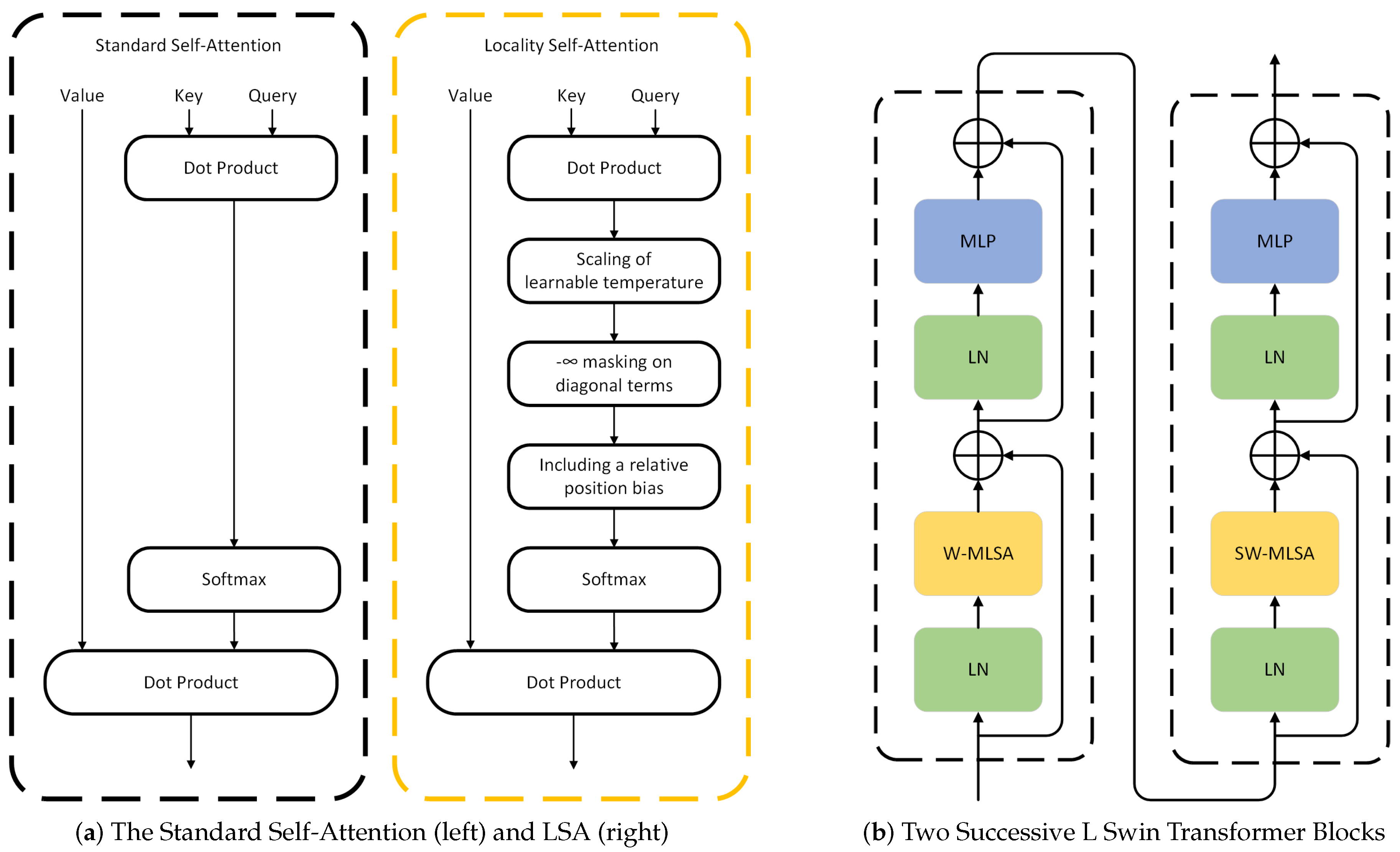
2.3.3. Locality Self-Attention

The core of the Locality Self-Attention Mechanism (LSA) consists of diagonal masking and learnable temperature scaling. Figure 3a demonstrates the difference between the standard self-attention mechanism and the locality self-attention used in the SL-Swin model. Figure 3b shows how LSA is applied in successive Swin Transformer blocks to form the L Swin Transformer blocks. The W-MLSA and SW-MLSA in the two successive Swin Transformer blocks shown in Figure 3b denote window-based multi-head locality self-attention using regular and shifted window partitioning configurations, respectively; an L indicates where the LSA is applied.

The standard self-attention computation of general ViTs operates as follows. In the beginning, the Query, Key, and Value are obtained by applying a learnable linear projection to each token. Next, the similarity matrix R, which represents the relation between tokens, is calculated through the dot product operation of the Query and Key. The diagonal and off-diagonal components of R represent self-token and intertoken relations, respectively:

$$R=Q{K}^T$$

(6)

Here, Q and K denote learnable linear projections for Query and Key. Afterwards, the diagonal masking forces $-\infty$ on the diagonal components of R to emphasize intertoken relations by essentially excluding self-token relations from the following computation. This forces the model to concentrate more on other tokens rather than intertoken relations. The diagonal masking is formulated as follows:

$$R^M=\left\{\begin{array}{c}{R}_{i,j}\left(i\ne j\right)\\ -\infty \left(i=j\right)\end{array}\right.$$

(7)

where $R^M$ represents the masked similarity matrix, and i and j respectively indicate the row and column index of the similarity matrix R.

After diagonal masking, learnable temperature scaling is applied to allow the model to determine the softmax temperature by itself during the learning phase. As the attention mechanism is used in the SW-MSA and SW-MSA of the backbone Swin Transformer, we included a relative position bias B to sustain the backbone architecture. Finally, the attention score matrix is attained through the softmax operation, with the self-attention matrix acquired using the dot product of the attention score matrix and the Value:

$$Attention\left(Q,K,V\right)=softmax\left(\frac{R^M}{\tau }+B\right)V$$

(8)

where V is the learnable linear projection of the Value and $\tau$ is the learnable temperature.

2.4. Pseudo-Labeling

As ground truth labels (the onset, offset, and apex frame indices) only provide the status label of a given frame, which does not correspond to the optical flow features that carry motion information between frames, we utilized the pseudo-labeling approach presented by Liong et al. [25] in the training phase. First, the sliding window $W_i$ which denotes the interval $[F_i,F_{(i+k)}]$ is scanned across each video. Subsequently, the function g is applied to acquire the pseudo-label $\widehat{l}$ for each sliding window calculated from the Intersection over Union (IoU) method, which compares the sliding window W and the ground truth interval $W_{grondTruth}$:

$$W_{grondTruth}=\left[F_{onset},F_{offset}\right]$$

(9)

$$IoU=\frac{W\cap W_{grondTruth}}{W\cup W_{grondTruth}}$$

(10)

$$g\left(IoU\right)=\left\{\begin{array}{c}0,IoU\le 0\\ 1,IoU>0\end{array}\right.$$

(11)

Finally, the pseudo-label sequence $\widehat{L}=\{{\widehat{l}}_i,fori=F_{start},\dots ,F_{(end-k)}\}$ together with the preprocessed optical flow features were used to train the SL-Swin model. The process of pseudo-labeling is shown in Figure 4.

2.5. Spotting

The predicted scores sequence S of every video was smoothed to obtain the smoothed scores sequence $\widehat{S}$:

$${\widehat{s}}_i=\frac{1}{2k}\sum _{j=i-k}^{i+k-1}{s}_{j}fori=F_{(start+k)},\dots ,F_{(end-k+1)}$$

(12)

where $s_j$ and ${\widehat{s}}_i$ indicate the j-th value in the raw predicted scores sequence S and i-th value in the smoothed score sequence $\widehat{S}$, respectively. In the smoothing scheme, the interval $[F_{(i-k)},F_{(i+k-1)}]$ of the current frame $F_i$ is averaged. Each smoothed score value ${\widehat{s}}_i$ now represents the probability of the current frame $F_i$ being within an expression interval.

Finally, we employed the standard threshold and peak detection technique from [28] to spot the peaks in each video, with the threshold defined as

$$T={\widehat{S}}_{mean}+t\times \left({\widehat{S}}_{max}-{\widehat{S}}_{mean}\right)$$

(13)

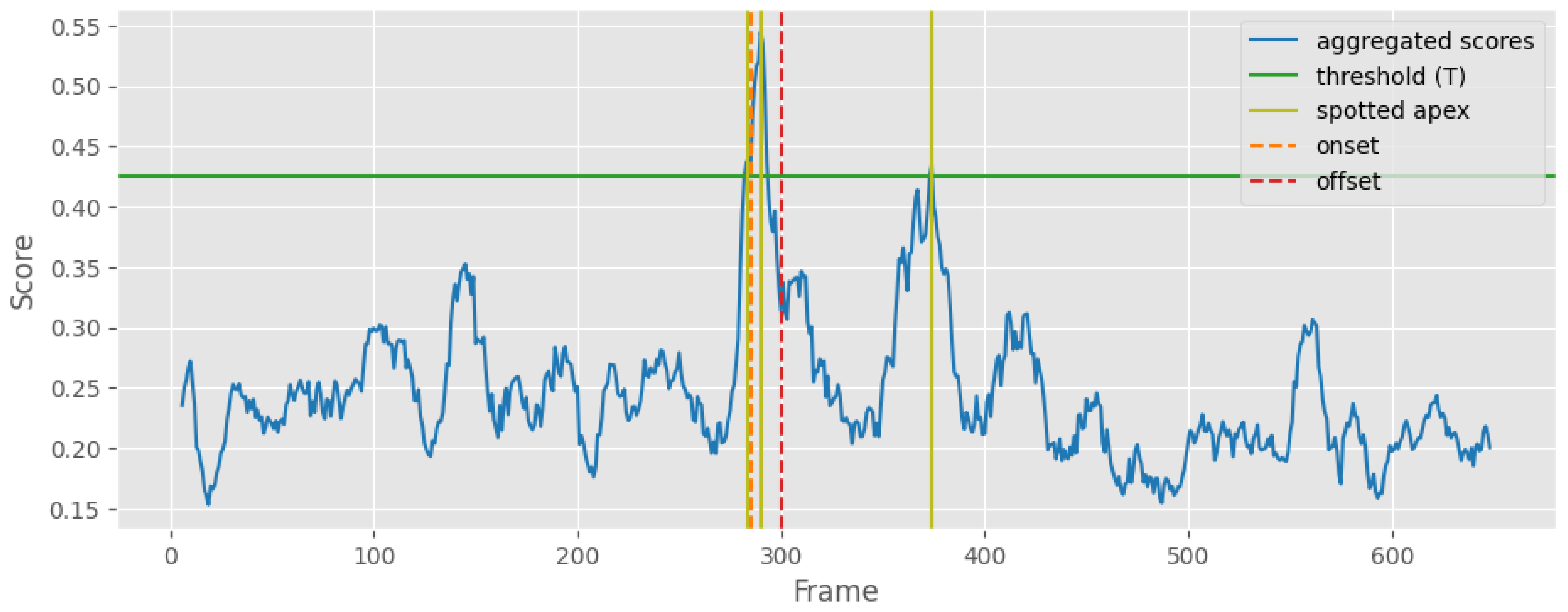
where ${\widehat{S}}_{mean}$ and ${\widehat{S}}_{max}$ are the average and maximum value of the smoothed scores sequence $\widehat{S}$, respectively, and t is a percentage parameter used for tuning that ranges from 0 to 1. We detected the local maximum (with the minimum distance of k between peaks) to find the peak frame ${\widehat{F}}_p$ with the peak value ${\widehat{s}}_p$. The spotted peak frame ${\widehat{F}}_p$ was considered as the spotted apex frame and the spotted onset–offset interval $[F_{(p-k)},F_{(p+k)}]$ for evaluation was obtained by extending k frames. An example of the spotting process is demonstrated in Appendix C.

3. Results

In this study, we conducted experiments on both the MEGC 2022 and MEGC 2021 spotting tasks. Note that the model was implemented separately for training and inference of macro- and micro-expressions. The code has been made available publicly to encourage community use in Appendix A.

3.1. Evaluation Datasets

3.1.1. MEGC 2022 Dataset

MEGC 2022 provides a single unseen test dataset for evaluation. The dataset consists of ten long videos: five clips cropped from different videos in CAS(ME)${}^3$ [33] and five long videos from SAMM (the SAMM Challenge dataset) [34], which have frame rates of 30 fps and 200 fps, respectively.

Briefly, CAS(ME)${}^3$ provides around 80 h of videos with over 8,000,000 frames, including 3490 manually labeled macro-expressions and 1109 manually labeled micro-expressions. The clips from such a large dataset allow validation of effective expression spotting approaches without database bias. Additionally, CAS(ME)${}^3$ uses the mock crime paradigm along with physiological and voice signals to elicit micro-expression with high ecological validity, contributing to practical expression analysis.

SAMM, the origin of the SAMM Challenge dataset, has the largest amount of different ethnicities and age distributions, as well as the highest resolution, among all current publicly available expression datasets. Therefore, the five long videos from this dataset are more representative of a given population, and expressions induced from different people acquired in a non-laboratory environment containing varieties of emotional responses can be considered.

Consequently, to a certain extent, the results from these ten long videos reflect how efficiently an approach is able to spot expressions in real-world scenarios. However, ground-truth labels have not been released for these two test datasets, and evaluation needs to be conducted using the grand challenge system (https://megc2022.grand-challenge.org, accessed on 8 June 2023).

3.1.2. MEGC 2021 Datasets

MEGC 2021 provides two datasets for training and evaluation: CAS(ME)${}^2$ [35] and SAMM Long Videos [32,36]. Both datasets are fully annotated with onset, apex, and offset by professional coders.

Briefly, CAS(ME)${}^2$, the first dataset to contain both macro-expressions and micro-expressions from the same participants and under the same experimental conditions, includes 98 long videos consisting of 300 macro-expressions and 57 micro-expressions captured from 22 subjects. The resolution of this dataset is 640 × 480 and the frame rate is 30 fps. In addition, the dataset relied on an elicitation procedure that has been proven valid in previous work [37] to induce both macro-expressions and micro-expressions, and participants were asked to neutralize their facial expressions while watching emotion-evoking videos. These two procedures mean that all expression samples are ecologically valid and dynamic. In addition, the participants were asked to watch the videos of their recorded facial expressions and offer a self-report on each expression, which excludes emotion-irrelevant facial movements and ensures pure expression samples. In our experiments conducted on CAS(ME)${}^2$, frames from the video “0503unnyfarting” of the subject “s23” in the “rawpic” folder had no annotation in the Excel file; consequently, we excluded this video and used only the other 298 macro-expressions in our experiments.

SAMM Long Videos is an extension of SAMM [34] with 147 long videos (consisting of 343 macro-expressions and 159 micro-expressions) captured from 32 subjects. Compared to CAS(ME)${}^2$, the SAMM Long Videos dataset has a higher resolution (2040 × 1088) and frame rate (200 fps) as well as more long videos and expressions, particularly micro-expressions. Additionally, labels of macro-movements and micro-movements are provided in this dataset to indicate both facial expressions and other facial movements such as eye blinks. However, twelve macro-expression samples has to be omitted in our experiments due to ambiguous onset annotation.

3.2. Performance Metrics

We used the standard Intersection over Union (IoU) method for evaluating our spotting approach, consistent with the spotting tasks in MEGC 2021 and MEGC 2022. We compared the spotted interval $W_{spotted}$ with the ground-truth interval $W_{grondTruth}$, and considered a True Positive (TP) to be when the following condition was met:

$$\frac{W_{spotted}\cap W_{grondTruth}}{W_{spotted}\cup W_{grondTruth}}\ge J$$

(14)

with J set to 0.5. Otherwise, the spotted interval $W_{spotted}$ was considered a False Positive (FP) result. In addition, a $W_{grondTruth}$ that failed to be spotted was considered a False Negative (FN). Subsequently, we calculated the Precision and Recall. The Precision, obtained based on Equation (15), measures the accuracy of an approach in identifying a spotted interval as an expression interval, while the Recall, calculated from Equation (16), indicates how accurately an approach is able to identify the spotted intervals that actually contain expressions out of all spotted intervals.

$$Precision=\frac{TP}{TP+FP}$$

(15)

$$Recall=\frac{TP}{TP+FN}$$

(16)

Finally, we used the F1-score to evaluate the performance of the macro-Expression (MaE) and micro-Expression (ME) spotting approaches as well as the overall analysis. Notably, the approaches and evaluations for MaE and ME spotting were conducted separately.

$$\mathit{F1-score}=\frac{2\times Precision\times Recall}{Precision+Recall}$$

(17)

3.3. Settings

In the experiments using the MEGC 2022 datasets, the model was trained on CAS(ME)${}^2$ and SAMM Long Videos, respectively, and evaluated on CAS(ME)${}^3$ and SAMM Challenge. The spotted MaE and ME intervals were then submitted to the grand challenge system (https://megc2022.grand-challenge.org) to obtain the results. For MEGC 2021, we employed leave-one-subject-out (LOSO) cross-validation to eliminate subject bias and ensure that all samples were evaluated.

The k parameter (half of the average length of an expression interval) was computed to be $\{6,18\}$ for CAS(ME)${}^2$ and CAS(ME)${}^3$ and to be $\{37,169\}$ for the SAMM Long Videos and SAMM Challenge (a smaller value for micro-expressions and larger value for macro-expressions). For peak detection in the spotting procedure, we selected $t=0.60$ for both MEGC 2022 and MEGC 2021.

Note that there are different versions of the backbone model Swin Transformer. We selected the tiny version, called Swin-T, as the backbone of our model, which is about $0.25\times$ the model size and computational complexity of the base Swin Transformer (Swin-B). We called the model used in our experiments SL-Swin-T, indicating that SPT and LSA were applied to the Swin-T backbone. We used a window size of $M=7$, the query dimension of each head was set to $d=32$, and the expansion layer of each MLP was $\alpha =4$. The other architecture hyperparameters of the SL-Swin-T model were the channel number of the hidden layers in “Stage 1” $C=96$ and layer numbers $=\{2,2,6,2\}$.

In all our experiments, the model was trained on an NVIDIA GTX 2080 Ti. The number of epochs was set to 25, and we applied the SGD optimizer with a learning rate of $5\times {10}^{-4}$. In the training phase, we sampled one of every two non-expression frames. To address small sample size problem during micro-expression training, we applied data augmentation techniques including Gaussian blur (with a kernel size of $7\times 7$), adding random Gaussian noise ($N(0,1)$), and horizontal flipping.

3.4. Permormance

The results of our approach on the MEGC 2022 spotting task are shown in

Table 1. Performance comparison of our approach on the MEGC 2022 spotting task.

Approaches	CAS(ME)${}^3$ Challenge			SAMM Challenge			Overall
	Precision	Recall	F1-Score	Precision	Recall	F1-Score	Precision	Recall	F1-Score
Baseline [15]	0.4000	0.1111	0.1739	0.0845	0.1935	0.1176	0.1235	0.1493	0.1351
Swin-T	0.1521	0.1944	0.1707	0.6380	0.0967	0.0769	0.1075	0.1492	0.1250
Ours	0.1944	0.1944	0.1944	0.0689	0.1290	0.0898	0.1170	0.1641	0.1366

.

Table 2. Performance comparison (F1-score) of our approach against other models on the MEGC 2021 spotting task.

Dataset	CAS(ME)${}^2$			SAMM Long Videos
Approaches	Macro	Micro	Overall	Macro	Micro	Overall
Traditional Approaches
He et al. [38]	0.1196	0.0082	0.0376	0.0629	0.0364	0.0445
Zhang et al. [8]	0.2131	0.0547	0.1403	0.0725	0.1331	0.0999
He et al. [39]	0.3782	0.1965	0.3436	0.4149	0.2162	0.3638
Deep Learning Approaches
Baseline [15]	0.2145	0.0714	0.1675	0.1595	0.0466	0.1084
Yand et al. [7]	0.2599	0.0339	0.2118	0.3553	0.1155	0.2736
Yu et al. [40]	0.3800	0.0630	0.3270	0.3360	0.2180	0.2900
Liong et al. [25]	0.2410	0.1173	0.2022	0.2169	0.1520	0.1881
Liong et al. [41]	0.4104	0.0808	0.3250	0.2810	0.1310	0.2380
Ours	0.2236	0.0879	0.1824	0.1675	0.1044	0.1357

compares the results of our approach to other approaches, which are categorized into traditional approaches and deep learning approaches. A discussion of the results as well as the details of the MEGC 2021 spotting task are provided in the Discussion section.

4. Discussion

4.1. MEGC 2022 Spotting Task

Table 1 shows the results of our approach on the MEGC 2022 spotting task. Our model outperformed the baseline approach, obtaining an F1-score of 0.1944 on the CAS(ME)${}^3$ dataset and an overall F1-score of 0.1366. Examining the results for the CAS(ME)${}^3$ dataset in detail, our approach achieves a higher recall while having a lower precision. This effect is attributed to the smaller number of false spotted intervals, resulting in a smaller number of False Negatives (FNs). Compared to the approach that uses the tiny version of the Swin Transformer backbone without SPT and LSA, recorded in the table as Swin-T, our approach (SL-Swin-T) presents better results across all indicators, which indicates that the application of SPT and LSA improves the model’s generalization ability.

4.2. MEGC 2021 Spotting Task

For comparison, Table 2 shows the results of our approach on the MEGC 2021 spotting task against other approaches, which are categorized into traditional and deep learning approaches. Overall, our approach outperforms the baseline, demonstrating that Transformer-based models can achieve competitive performance compared to models based on Convolutional Neural Networks.

Our approach outperforms all traditional approaches except for the state-of-the-art approach proposed by He et al. [39]. Among the deep learning approaches, our approach remains competitive, especially for ME spotting on the CAS(ME)${}^2$ dataset, with an F1-score of 0.0879, behind only the approach proposed by Liong et al. [25], which spots a larger amount of TPs. By examining the details in

Table 3. Detailed results of the SL-Swin-T model on the MEGC 2021 spotting task.

Dataset	CAS(ME)${}^2$			SAMM Long Videos			Overall
Expression	MaE	ME	Overall	MaE	ME	Overall
Total	298	57	355	331	159	490	845
TP	70	12	82	52	33	85	167
FP	258	204	462	238	440	678	1140
FN	228	45	273	279	126	405	678
Precision	0.2134	0.0556	0.1507	0.1793	0.0698	0.1114	0.1278
Recall	0.2349	0.2105	0.2310	0.1571	0.2075	0.1735	0.1976
F1-score	0.2236	0.0879	0.1824	0.1675	0.1044	0.1357	0.1552

, on the CAS(ME)${}^2$ dataset, the amount of FP we obtained is comparable, which attributes to the competent Overall Precision of this dataset.

4.3. Ablation Studies

We conducted experiments to provide a thorough examination of our approach, focusing on network construction, the labeling function, and feature sizes. Experiments were conducted on the CAS(ME)${}^2$ dataset using similar settings as those used for the MEGC 2021 spotting task.

4.3.1. Network Architecture

To evaluate the effectiveness of the self-attention mechanism, SPT, and LSA, we conducted a similar experiment using different combinations of network architecture, SPT, and LSA. Here, S indicates that SPT was applied to the network, L indicates that LSA was applied to the network, and SL indicates that both SPT and LSA were applied.

Table 4. Performance comparison (F1-score) of our model (SL-Swin-T) against other Transformer-based models.

Network Architecture	CAS(ME)${}^2$
	MaE	ME	Overall
ViT-B	0.2125	0.0158	0.1415
SL-ViT-B	0.2071	0.0940	0.1738
Swin-T	0.2110	0.0783	0.1663
S-Swin-T	0.2351	0.0749	0.1685
L-Swin-T	0.2378	0.0493	0.1765
SL-Swin-T	0.2236	0.0879	0.1824

displays the experimental results of the various network architectures. According to our findings, SPT and LSA together enhance the network’s performance on small-size datasets, specifically ME spotting on CAS(ME)${}^2$. It is worth noting that the Swin-T model and the models based on it have only approximately $0.25\times$ the size and computational complexity of the ViT-B and the SL-ViT-B models.

4.3.2. Labeling

An ablation study was carried out on the original labeling and pseudo-labeling functions to investigate their impact on spotting when modeling the task as a regression problem. We set the parameter $t=0.60$ and compared the result on the SL-Swin-T model using original labeling and pseudo-labeling separately. The results are shown in

Table 5. Performance comparison of pseudo-labeling and original labeling.

Dataset		CAS(ME)${}^2$
Expression	Labeling	TP	FP	FN	Precision	Recall	F1-Score
MaE	Original	71	264	227	0.2119	0.2383	0.2243
	Pseudo	70	258	228	0.2134	0.2349	0.2236
ME	Original	14	262	43	0.0507	0.2456	0.0841
	Pseudo	12	204	45	0.0556	0.2105	0.0879
Overall	Original	85	526	270	0.1391	0.2394	0.1760
	Pseudo	82	462	273	0.1507	0.2310	0.1824

. It can be observed that applying pseudo-labeling reduces the amount of False Positives (FPs), resulting in enhanced Precision and F1-score, particularly in the overall analysis.

4.3.3. Feature Size

In our approach, the SL-Swin-T model takes optical flow features $(u,v,|ϵ\left|\right)$ of size $(42,42,3)$ as input. Due to patch merging in each stage of the model, the feature map is downsampled by a rate of 2, leading to only $\frac{42}{48}\times \frac{42}{48}=0.875\times 0.875$ pixels from the original optical flow features in “Stage 4”. To accommodate the windowing configuration, we apply padding when the feature map size is not an integer multiple of the window size $M=7$. Thanks to this hierarchical architecture and self-attention computation within windows, the Swin Transformer has linear computational complexity with respect to image size. This makes the Swin Transformer suitable for processing high-resolution images, in contrast to previous Transformer-based architectures which produce feature maps of a single resolution and have quadratic complexity. Hence, we doubled the hyperparameters in feature extraction and preprocessing, resulting in the size of $(u,v,|ϵ\left|\right)$ being $(84,84,3)$ and allowing $\frac{84}{48}\times \frac{84}{48}=1.75\times 1.75$ pixels from the original optical flow features in “Stage 4” of the model. The hyperparameters for the SL-Swin-T model and training configuration remained unchanged and the spotting parameter t was set to 0.60 for comparison. The experimental results for ME spotting are presented in

Table 6. Performance comparison of the size of optical flow features.

Dataset		CAS(ME)${}^2$
Expression	Features of Size	TP	FP	FN	Precision	Recall	F1-Score
ME	(42, 42, 3)	12	204	45	0.0556	0.2105	0.0879
	(84, 84, 3)	13	190	44	0.0640	0.2281	0.1000

, demonstrating that the model performs better across all indicators, with particularly strong results in terms of the F1-score.

4.4. Limitations and Future Work

While our approach demonstrates promising results, we recognize its limitations and potential areas for future research. First, although we built our model using the tiny version of the Swin Transformer, it is nevertheless considerably larger and more complex than CNN-based models, which poses challenges when reproducing results and makes LOSO experiments more time-consuming. In particular, compared to the ME spotting experiment on the SAMM Long Videos dataset in the MEGC 2021 spotting task, the MaE spotting experiment requires an additional week to carry out. Moreover, while traditional approaches can provide detailed explanations for the occurrence of an expression, our twelve-layer model functions roughly as a black box. Therefore, it is essential to find an effective method for interpreting what the model learns from the training data. This can help to improve the feature extraction and preprocessing phases.

Second, our model’s performance on expression spotting is not as appealing as it is on other tasks. This may be attributed to its sensitivity to training configurations such as batch size, number of epochs, and learning rate. Hence, we assume that our tuning does not fully show the advantages of applying both SPT and LSA. Consequently, in order to optimize model performance we suggest fine-tuning techniques such as pretraining the model on other datasets or experimenting with different loss and optimization functions specifically designed for small datasets.

Third, although increasing the input feature size to $(84,84,3)$ has been proven to enhance model performance, this remains much smaller than the Swin Transformer’s assumed input size of $224\times 224$. Consequently, it is reasonable to anticipate that utilizing a larger input resolution may further improve the results. However, it is notable that the larger input resolution means higher computation complexity, requiring advanced hardware and more time for experiments. Simultaneously, employing models with a larger backbone, such as the small version of Swin Transformer (Swin-S) or the base version of Swin Transformer (Swin-B), may lead to higher performance on high-resolution inputs, though with higher computational costs. As such, it is crucial to strike a balance between performance gains and available resources.

5. Conclusions

In this paper, we propose a deep learning approach that uses a Transformer-based model called SL-Swin, which incorporates Shifted Patch Tokenization and Locality Self-Attention into the backbone Swin Transformer network, to predict a score indicating the probability of a frame being within an expression interval by analyzing optical flow features. The results demonstrate that our approach is highly capable on both the MEGC 2022 and MEGC 2021 spotting tasks, indicating the potential of our approach to accurately identify expressions on small datasets and highlighting the practicality of our approach in scenarios where large-scale labeled expression datasets may not be readily available. Our evaluation outcomes surpass the MEGC 2022 spotting baseline result, obtaining an overall F1-score of 0.1366. Additionally, our approach performs well on the MEGC 2021 spotting task, achieving F1-scores of 0.1824 on CAS(ME)${}^2$ and 0.1357 on SAMM Long Videos. Our work shows the potential of Transformer-based models to achieve better performance with increasing data volumes. In the future, researchers could easily deepen the proposed model, increase its size, or apply other techniques designed for small datasets in order to enhance its spotting performance. Furthermore, owing to the challenges in the ME annotation process, researchers might consider implementing self-supervised learning to enable the network to learn more meaningful latent representations.