1. Introduction
Frequently, mobile robots are deployed with the primary objective of surveying their surroundings to gather valuable information, such as creating a map or identifying the position of an object of interest. Additionally, they can perform a detailed analysis of the environment’s condition either through the direct reconstruction of surfaces or by assessing the quality of its components to determine its overall health or status. Many of the environments in which robots are deployed are complex environments, such as multi-story buildings with connecting staircases, uneven surfaces, etc. In addition, robots are subject to kinematic constraints and, in many applications, the environment in which they are located is an environment about which there is very little information or even unknown, and the combination of these aspects can make exploration a difficult task for a ground robot. For this reason and the recent decline in their price, there has been a great increase in the use of aerial robots (commonly known as drones), particularly mini-drones and micro-drones. Despite their rather limited autonomy, their versatility has made them very attractive in both the industrial and military markets as well as to the public. Common areas of application include the agricultural sector [
1], search and rescue [
2], cultural heritage [
3], and industrial inspection [
4].
In particular, they have become an increasingly popular tool for agriculture over the past few years. They offer a cost-effective and efficient way to monitor crops, assess crop health, and gather data for precision agriculture. Drones can cover large areas quickly and capture high-resolution images and other types of data that can be analyzed to identify issues and make informed decisions about crop management. One of the main benefits of using drones for agricultural monitoring is the ability to gather data more frequently and at a higher resolution than is possible with other methods, such as satellite imagery or ground-based sensors. This allows farmers and agronomists to identify problems early and take action to mitigate them, improving crop yields and reducing costs. There are many different types of sensors and data-gathering equipment that can be attached to drones, including cameras, multispectral sensors, and thermal cameras. These can be used to gather a wide range of data, such as plant health, soil moisture levels, and pest and disease outbreaks. The data collected by drones can be used to create detailed maps and reports that can help farmers optimize their operations and make informed decisions about things such as irrigation, fertilization, and pest control. Summarizing, drones offer a valuable tool for monitoring and managing agriculture. They allow for the collection of high-resolution data over large areas, enabling farmers and agronomists to identify problems early and take action to improve crop yields and reduce costs.
Apart from the agricultural sector, many other industrial applications could benefit from drone technologies following the Industry 4.0 paradigm. Drones can be efficiently used for activities such as monitoring and inspection in confined spaces where human personnel has limited access [
5], or for inventory generation [
6] where their speed and maneuverability can reduce overall timing and required resources.
Independently from the task to accomplish, efficient exploration of the environment is essential. To inspect an environment in an automated manner, it is necessary to have a plan of the path the robot will need to take within the environment. Strategies for planning trajectories are commonly known as the Path-Planning Problem (PPP). Given the starting and ending positions of the robot, the goal is to find a path that leads the robot from the initial position to the final position while minimizing some costs and avoiding collisions with possible obstacles present along the path. Depending on the specific application, the cost to be minimized can be the time, the number of direction changes, the number of braking, or the energy consumption. In PPP, there are no constraints regarding the number of passages that can be made over a certain area. In contrast, the purpose of many applications is to completely explore an environment while avoiding inspecting an area that has already been inspected to reduce energy consumption and at the same time to make the robot return to its initial position at the end of the exploration to make a safe landing (in the case of UAVs) or to allow easy recovery of the robot by an operator.
Coverage Path Planning (CPP) is the problem of finding a path (if any) from a given point to itself that passes through every part of the area of interest, avoiding collisions and minimizing passes over areas already examined. This definition leads back to the well-known Traveling Salesman Problem (TSP), in which the area to be inspected is modeled as a set of nodes in a graph (i.e., waypoints), and a path is a sequence of arcs that begins and ends at the same node. As is well known, finding the Hamiltonian cycle optimum in a graph is part of the NP-hard class of problems; consequently, the computational cost of solving large instances is often too high for the requirements imposed by the application.
Heuristic and meta-heuristic algorithms have polynomial complexity and are useful since they can provide “good” admissible solutions to the CPP problem at a low computational cost. In addition, to decompose the problem into simpler subproblems, most of the algorithms for CPP use geometric decomposition techniques: the area is partitioned into several sub-areas, called cells, which are easily explored with simple Back and Forth trajectories. Thanks to these geometric decomposition techniques, it is also natural to model situations in which there is a fleet of aerial robots that has to accomplish the mission, since it is possible to assign a defined set of cells to each of them and finally merge the information collected at the end of the explorations.
In this context, the contribution of this manuscript aims at proposing a solution for the common problem of inspection of an area or surface with a robot. In particular, starting from an analysis of classical methods for generating navigation waypoints and performing CPP, an algorithm is selected as the basis for the presented approach. The path generated by the reference algorithm is then extended to account for the dynamics of the robot proposing an approach intended to save memory consumption and allow for path generation at different levels of detail. A test system, comprising an unmanned aerial vehicle, is presented complete with a simultaneous localization and mapping (SLAM) [
7] algorithm working both in outdoor and indoor scenarios. Lastly, starting from the mathematical model of the UAV, a Model Predictive Control (MPC) is designed for tracking the previously generated smooth coverage trajectory.
Summarizing, this work proposes the following:
An algorithm to generate waypoints given an arbitrary enclosing polygon;
A comparison of CPP state-of-the-art methods;
A smoothing method for a generated trajectory that allows changing the level of details of trajectory segments and that reduces the overall memory footprint;
A robot localization algorithm combining Lidar SLAM and GPS positioning to solve for pose estimation in both indoor and outdoor scenarios;
The implementation of a nonlinear MPC control that allows for generating optimal control inputs to a UAV considering state and input constraints.
The main result of the research is the flight-time reduction due to the proposed smoothing approach. Battery duration is probably the main issue when using an aerial vehicle, and a time reduction in the overall flight time favors the endurance of UAVs.
The remaining manuscript is structured as follows. In
Section 2, the state-of-the-art regarding CPP and UAVs applications is presented.
Section 3 introduces the proposed methods. In
Section 4, the test system hardware and software components are discussed.
Section 5 is dedicated to the control system and the experimental evaluations. A conclusion section summarizes the contribution and presents future activities.
2. Related Works
Many researchers have studied the problem of planning trajectories to cover spaces. Comprehensive surveys on the most promising algorithms [
8] and on UAV applications [
9] can be found in the recent literature. It emerges that most of the algorithms developed in recent years use some kind of geometric decomposition to make the problem more tractable. Ost [
10] examined different types of trajectories and area decomposition and found that the Back and Forth trajectory without area decomposition had the best results for a single UAV performing offline path planning. Driscoll [
11] developed an offline algorithm that can accurately cover an agricultural field in O(n2). Valente [
12] studied two meta-heuristic approaches: Harmony Search (HS) [
13] and Ant Colony Optimization (ACO) [
14] for CPP and found that ACO was the best approach for both online and offline systems in terms of path length and the number of changes of direction. An original approach to the solution of the TSP is given by Brocki in [
15], where he employs a modified Self-Organizing Map (SOM) [
16]. The purpose of the SOM technique is to represent the model of a map with a lower number of dimensions while maintaining the relations of similarity of the nodes contained in it. The presented approach substitutes the classical grid representation with a circular array of neurons where each node is only conscious of the neurons in front of and behind it. The convergence is assured by introducing a learning rate parameter with decay in a similar way to the Q-Learning approach.
To be able to make decisions about actions to be taken during exploration, it is often necessary to construct a map of the environment. Avellar et al. [
17] proposed an algorithm for covering space to obtain a series of partially overlapping images of the underlying terrain, using a fleet of fixed-wing drones. Each drone is equipped with a downward-facing camera, and the altitude is adjusted based on the minimum resolution required. Avellar et al. modeled the area (which must either be convex or the convex envelope of a nonconvex area) as a graph and transformed the original problem into a Vehicle Routing Problem (VRP). VRP is a generalization of TSP in which the goal is to find a set of disjoint paths, each of them traveled by a vehicle, that traverses all nodes exactly once. The goal of the algorithm is first, to find the number of drones that minimizes the time required to cover the area. Secondly, it is to calculate the path for each drone that covers its assigned waypoints at the minimum time. Di Franco and Buttazzo [
18] performed three experiments to evaluate and model the variations in the consumption of energy in different flight situations and proposed a cost function that, when minimized, provides the optimal speed at which the drone must travel to save energy, both in the case of constant and variable speed.
Ongoing research in coverage path planning for UAVs presents different approaches to improve the efficiency and effectiveness of UAV coverage operations, including multiobjective optimization techniques [
19], deep reinforcement learning [
20], and potential fields [
21]. According to a recent survey on the topic [
22], most approaches (nearly 80%) consider the velocity of the UAV as fixed, thus reducing the complexity of the problem [
23]. The methods considering timing issues are based on potential fields or bio-inspired algorithms such as ACO. This manuscript proposes an approach that exploits the full dynamics of UAVs and tackles the NP-Hard problem by trying to reduce the flight time for the full coverage of the environment.
3. Method
The primary objective of this work is to design a drone system able to obtain a sequence of photographs or scans that will allow the reconstruction of a certain environment as a whole at the lowest possible cost. The system receives as input the coordinates of the geographic boundaries corresponding to the area to be inspected. It then subdivides that area into rectangles partially overlapping, whose centers, called waypoints, represent the points at which the drone is to take the photographic snapshot of the underlying surface. Afterward, an intelligent algorithm should drive the drone to transit every single waypoint and return to the base minimizing the motion path length. Following the calculation of waypoints, the trajectory of the drone is then determined by solving the corresponding TSP in which the nodes of the graph represent the waypoints to be traversed at minimum cost, i.e., minimum length. There are two approaches chosen for solving the TSP: an evolutionary meta-heuristic based on Ant Colony Optimization (ACO) and a modified version of the Lin–Kernighan heuristics (LKH), i.e., a local search heuristic based on k-exchange dynamics.
A comparison of these approaches is presented, and the best one is selected as a basic CPP strategy. Starting from the solution provided by the best method, a smoothing algorithm is introduced to generate a smooth trajectory for the robot motion allowing for faster maneuvers and reduced memory consumption. At the same time, depending on the level of smoothing, the waypoints are resampled on the trajectory while still maintaining the full coverage properties necessary for the intended job.
3.1. Maximum Flight Height Computation
To guarantee the resolution
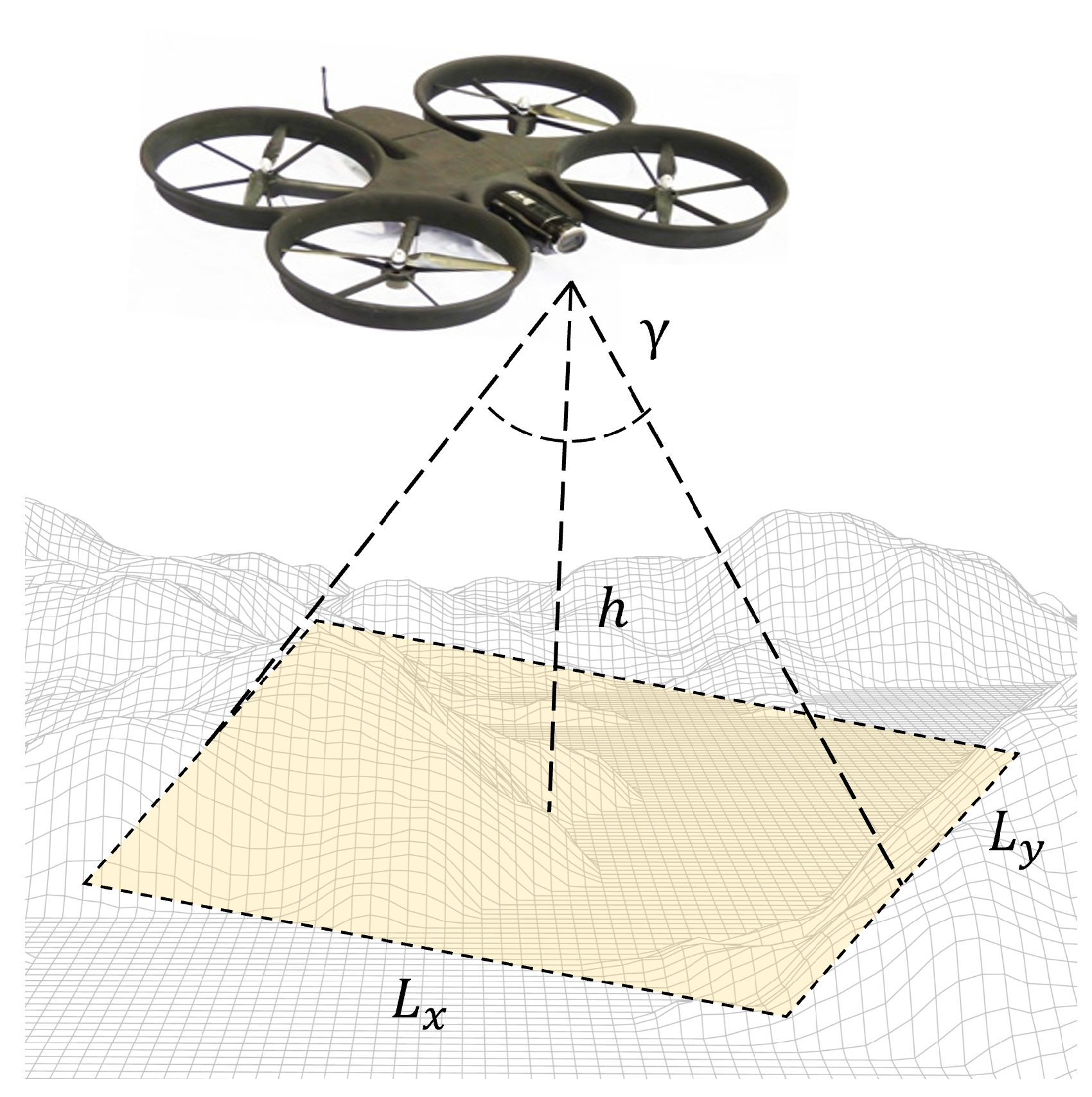
set by the user, it is necessary that the height of the drone is calculated accordingly. When the drone takes a photograph of the terrain below, the portion of the area framed by the camera is called the projected area. The size of the projected area depends on the field angle
of the camera and the flight height
h of the drone (
Figure 1).
The width
and length
of the projected area are calculated as follows:
with
representing the ratio between the horizontal and vertical resolution of the image sensor.
The spatial resolution
R, expressed in pixels per meter, is then given by the ratio of the width of the image
to the width of the projected area
:
Furthermore, to guarantee the resolution
, it is necessary to impose that
, and the flight height of the drone is then expressed as:
3.2. Waypoints Computation
Once the flight height is computed and the coordinates of the area to be inspected and obstacles are received, the waypoints can be calculated. The area must be divided into equal rectangles of dimensions
and
whose centers, the waypoints, represent all the points at which the drone has to take a photograph of the terrain below. Since the ultimate goal of the mission is to reconstruct a map formed by the union of the photographs taken, it is necessary that the shots are taken with a certain percentage of overlap. The waypoint calculation is completed in two stages. In the first step, a rectangle
B is constructed in such a way that the polygon representing the area to be inspected is internal to it. Next,
B is divided into equal-sized rectangles. Starting from the first rectangle in the lower-left corner, the first waypoint is located in the center of the rectangle itself. The process is iterated until the end of
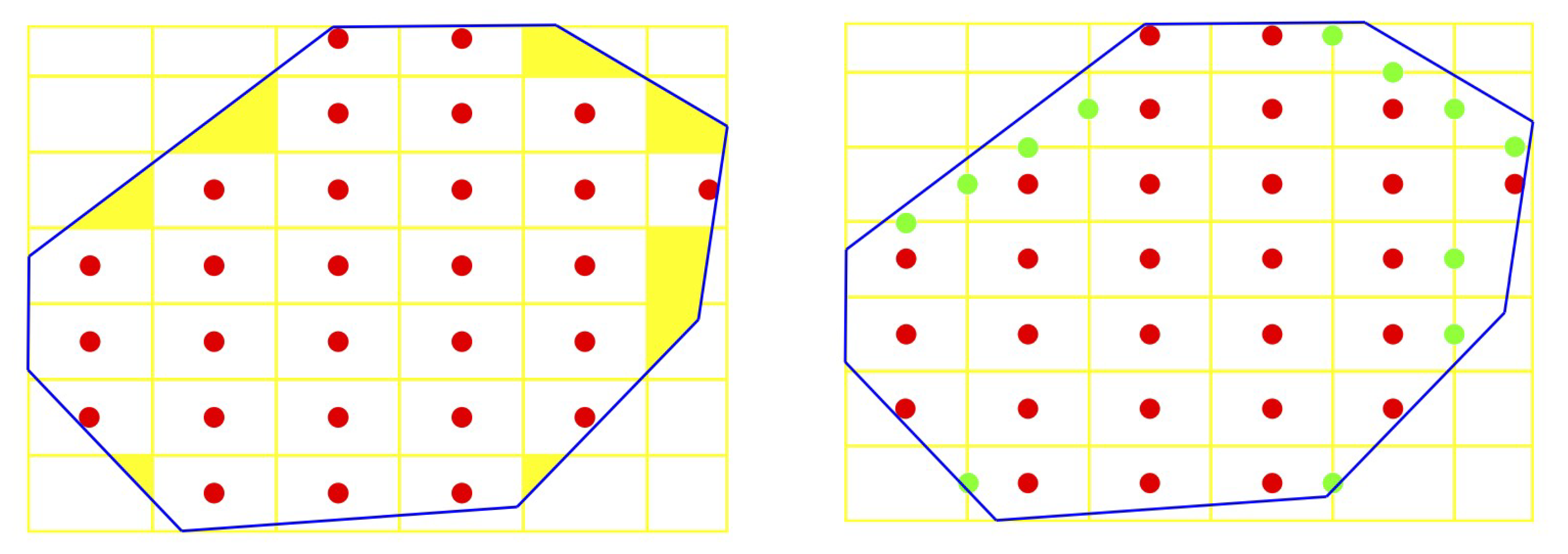
B is reached, and finally, the calculated waypoints found to belong in the area are placed into a list. At this point, it is likely that the waypoints just computed are not sufficient to ensure complete coverage of the area, as can be seen in the yellow areas in
Figure 2. For this reason, additional waypoints are inserted in a second phase to cover any areas that were not previously covered. The procedure consists in adding temporary waypoints in the middle of the edges of the uncovered regions. A test is performed on these augmented waypoints to verify if they belong to the inspection area, and accordingly, they are added to the waypoints list.
Once the coordinates of the waypoints have been obtained, it is necessary to proceed to the calculation of the trajectory to be carried out by the drone.
3.3. CPP Methods Analysis
The following paragraphs will discuss the two heuristics that were implemented to solve the TSP. A performance comparison of the methods has been conducted to select the winning algorithm as the base for the proposed CPP approach.
3.3.1. ACO
The Ant Colony Optimization algorithm is based on the behavior of ants, which by cooperating through pheromones can find the shortest path between a food source and their nest. When an ant moves, it releases on the ground a certain amount of pheromone. This hormone influences other ants, which will choose the path where its concentration is highest. The shorter the path is from the nest to the food source and from the latter to the nest, the higher the concentration of pheromone that subsequent ants will find on the ground, as the ant that has chosen the shorter path will return to the nest before the ant that has chosen a longer path. It is possible to formalize the above behavior by modeling the ants’ motion as a non-complete, undirected graph with a finite number of nodes.
The adopted implementation is the Ant System (AS) variant from the ACO [
24] library. In this variant, the next waypoint
j is selected starting from the current waypoint
i with a probability
computed as:
where
is the set of waypoints
w that are reachable from
i,
represents the amount of pheromone that is present on the arc
, and
is the distance heuristics of the arc.
A set of parameters needs to be chosen to properly use the ACO algorithm, and for such a purpose, a parameter search has been conducted within the following ranges:
in the range 0.3–5.0, which represents the influence of the pheromones.
in the range 4.3–10.3, which represents the influence of the heuristic information.
Q in the range 75–105, which is the total pheromone quantity on the best path found at each iteration.
in the range 0.1–0.7, which is the evaporation coefficient of the pheromone update.
in the range 1.3–7.3, which is the maximum pheromone value on the arcs at the beginning of the algorithm.
The number of ants in the range 2–8.
The number of iterations in the range 2–8.
The aim was to minimize both the trajectory length and the execution timing. The search resulted in the following optimal values: (; ; ; ; ; ; ), which have been used in the experimental trials. A result to be noted is that by increasing the number of ants or the number of iterations, shorter paths are found but with a significant increase in the execution time. For this reason, these two final values have been chosen to balance execution time and path length.
3.3.2. LKH
The second employed algorithm was implemented by Helsgaun in [
25] based on a modified version of the original Lin–Kernighan heuristic (LKH) [
26]. LKH belongs to local search heuristics methods, which, given an admissible solution, analyze solutions that are “close” to it in order to find the best match. Thus, starting from an admissible solution, in our case a Hamiltonian cycle, we analyze Hamiltonian cycles “similar” to the starting one. This technique is called k-exchange. The principle behind LKH is to perform, at each iteration,
k-exchange operations and evaluate whether it is convenient to continue with operations of (
k + 1)-
exchange. For large instances, performing the
k-exchanges on the whole graph would be unnecessarily wasteful. Therefore, for each node, candidate sets are created containing the arcs that, hopefully, through the
k-exchange can improve the value of the objective function. The creation of the candidate sets is based on the minimum spanning tree (MST) and
-nearness concepts [
27].
For the implementation of LKH, some parameter values have been tested, but default values appeared to be fine in general. Analyzing for instance the INITIAL_TOUR_ALGORITHM parameter, that is the algorithm that is used to compute the initial path, all the options give comparable results and, as such, the nearest neighbor algorithm has been selected for the testing, while the number of maximum k-exchanges has been set to 5 and the number of iterations has been set to 10, which provided a good trade-off between computational cost and path length.
3.3.3. Testing
Testing sessions on the algorithms’ performance have been conducted by simulation through the V-REP [
28] simulator. The software interface allows the user to interact with the simulation with custom scripts that could manage all the models within the created scenario. Performance tests of the AS and LKH algorithms were performed on 6 groups of instances, each consisting of 100 scenarios generated in a pseudo-random manner. The groups differ in increasing instance size, while they share the following characteristics of the employed camera: image size (
,
) = (4000, 3000) pixels, angle of the field
= 94.4 deg, aspect ratio
= 4/3, and of the methods: desired resolution
= 5 pixels/cm, horizontal overlapping
= 24%, vertical overlapping
= 20%. Tests were run on a computer with an Intel Pentium processor T4500 2.3 GHz on a Ubuntu 18.04 LTS operating system and GCC version 7.4.0.
The results of the testing instances concerning the path length and execution time of the methods are reported in
Table 1.
The first test was performed on 100 scenarios of sizes up to 50 × 50 m. The resulting number of waypoints was . The path calculated by LKH was 10.60% shorter than the one computed with AS. In addition, LKH turned out to be almost 6 times faster than AS. In each successive test, the scenario was increased by up to 10 × 10 m concerning the previous one, reaching 100 × 100 m in the final test. The number of waypoints increased as well in successive tests, reaching in the final run. The performance of the LKH method compared to AS resulted in a nearly 20% shorter trajectory and nearly 50 times faster execution. It turned out that while the mean path length obtained from both the methods increases linearly with the size of the area to cover and is comparable, considering the execution time, the LKH method increases linearly while the AS timing increases cubically.
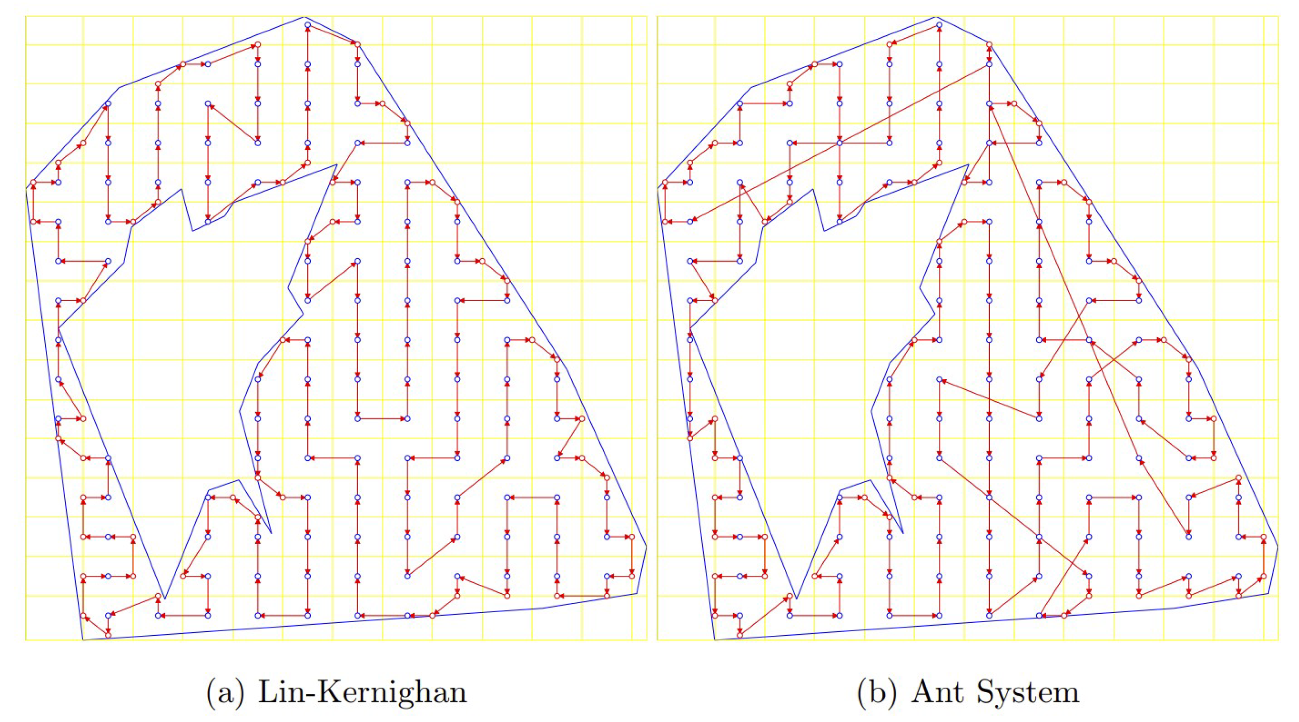
Figure 3 depicts a generated random scenario with dimensions nearly 75 × 75 m. According to Equation (
4), the value
cm is obtained, and the projected area size becomes
cm and
cm. Considering the chosen overlapping values, the final number of generated waypoints is 160. From the resulting path, as shown in
Figure 4, it is evident that the trajectory generated by LKH is shorter and avoids passing multiple times on the same cell.
The next paragraph will introduce an algorithmic procedure to arbitrarily smooth the obtained trajectory and reduce its memory footprint for embedded usage.
3.4. Toward a Smooth Trajectory
Any function, vector, or signal
f can be represented with a change of coordinate system as a linear combination of a set of axes
(basis):
where
are the coordinates of
f in the new system. By choosing a proper set of axes that are orthogonal to each other and that have more and more detail as
n increases, it is possible to exploit such representation to reduce the memory consumption for storing the path and to smooth the original trajectory, making it dynamically feasible. The coordinate system that fulfills the above-mentioned requirements is the trigonometric family of functions, namely the Fourier series:
Thanks to the perpendicularity between axes, to obtain the coefficients , it is sufficient to perform a dot-product between the vector f and the axes, such as when applying a rotation matrix to a vector. Rotating the vector f by the matrix , it is possible to transform its representation and store in memory just the coefficients and no more the function f. It is important to notice that higher-order axes represent the detailed structure of f, while its global structure is mostly projected into the lower order axes. In real-world scenarios where large amounts of data are produced to continuously explore the environment, it could suffice to store the global shape of a trajectory and discard the rest of the information. This can be obtained by storing a few of the coordinates and still obtaining good approximations of the original trajectories. In summary, there are two steps of storage reduction: the first is the transformation of the whole trajectory in a set of coefficients that could be compressed as well, for example considering that the last coordinates will be smaller than the first ones. The second source of reduction is the partial storage of the coefficients. Empirically testing shows that reducing the coefficient by 20–30% generates a quite unnoticeable difference in the majority of trajectories, while for many trajectories, it is possible to reduce the data over while still maintaining efficient results. A second aspect to consider is that by using trigonometrical functions and lower-order coefficients, the trajectory smooths out automatically removing trajectory points with discontinuous accelerations or jerks.
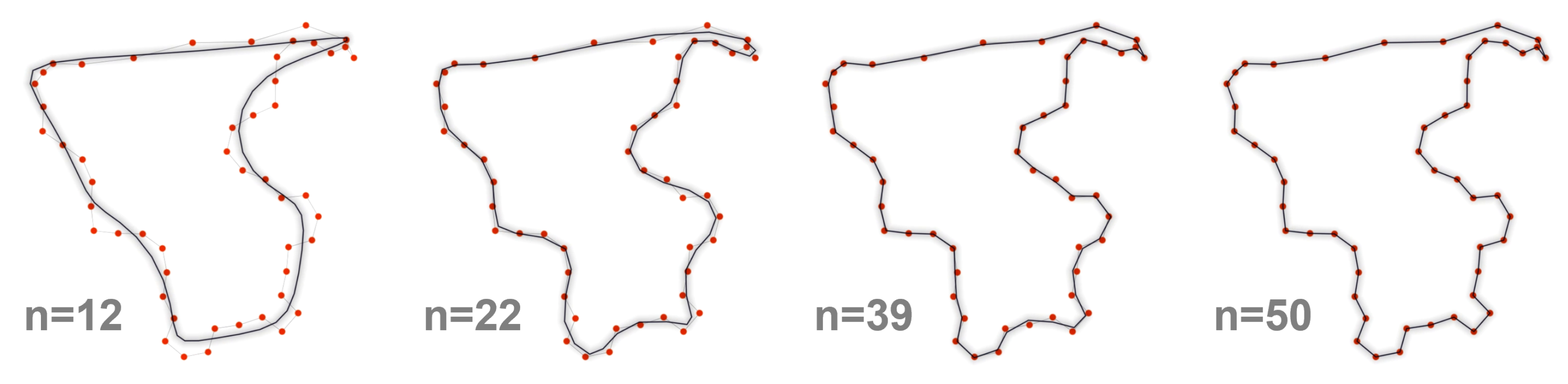
Figure 5 shows an example of the application of the presented method on a simple trajectory. The example trajectory is described by 50 waypoints and a traversal path generated with the LKH algorithm. The trajectory can be represented and stored in the navigation system with the full representation requiring 50 coefficients or with a reduced number of coefficients. It is possible to see that even with a small portion of the original data, the trajectory resembles the original one, and the result obtained with 39 coefficients is almost coincident with the full representation. Moreover, lower-order representations present smoother paths.
On the contrary, when there is the need to exactly pass on the specified waypoints but also the constraint of generating a dynamically smooth trajectory, it is possible to use the inverse Fourier transform and interpolate between the points to achieve a smooth path.
4. Unmanned Aerial System
The introduced algorithms are expected to be executed by an embedded processing unit on board an Unmanned Aerial Vehicle (UAV). The selected platform for the setup of the overall system and the testing session is a ducted fan quadrotor designed by Cyber Technology, The CyberQuad MAXI. It has four brushless motors suitable to be used in critical environments [
29] and a control board by MikroKopter that integrates a gyro, a three-axis accelerometer, a barometric sensor, and a compass. A camera is mounted on a pan–tilt base which automatically stabilizes the pan with respect to the horizontal direction and allows the user to adjust the tilt toward the desired direction. Two sonars (XLMaxSonarEZ4) and a Hokuyo laser (UTM-30LX) complete the sensor setup for indoor exploration, while a GPS module is used in outdoor scenarios.
Figure 6 shows the drone equipped with the sensors and the low-power control board based on the OMAP4430 processor from Texas Instruments (PandaBoard).
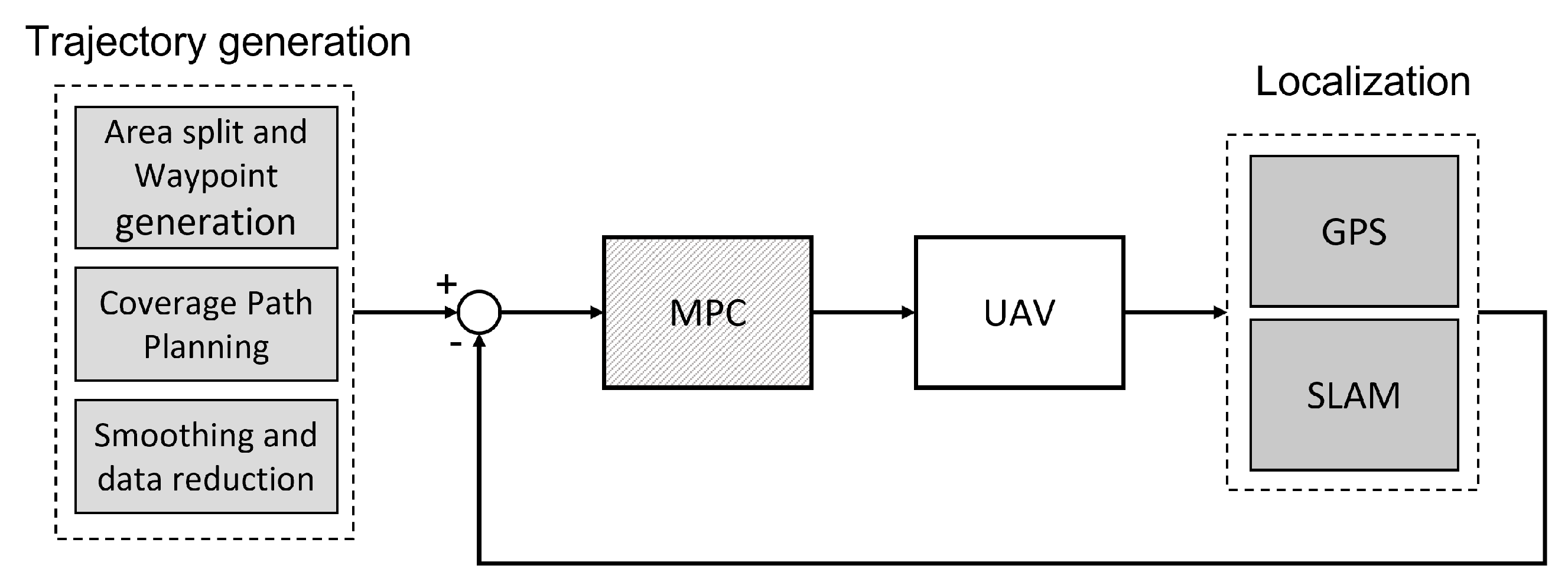
To maintain a stable flight during the inspection task, the system acquires information from the environment by means of a laser range finder (LRF) and two distance measuring sensors for indoor scenarios, while it employs a GPS antenna for outdoor inspections. This information is processed by a SLAM component that feeds the current position and the asset of the UAV to an MPC controller. The software components involved in the UAV control loop are shown in
Figure 7. The trajectory generation module that has been previously described is responsible for the generation of the reference trajectory for the quadrotor. The MPC controller (described in
Section 5) produces an optimal input to make the UAV follow the reference trajectory under specific constraints. The last element in the control loop is a localization module that starting from sensors readings produces estimations on the state of the robot. The next paragraph will discuss in detail this module.
Localization and State Estimation
The UAV is equipped with proprioceptive sensors that can measure local physical phenomena, such as the inertial sensors that measure the linear and rotational acceleration of the body. Other sensors extract information from the surrounding (exteroceptive sensors), such as ultrasound and laser sensors that can measure the distance from objects in the environment. Fusing these measurements, it is possible to obtain a good estimation of the UAV state (position and orientation in world coordinates). In the case of outdoor applications, the use of an additional global positioning system (GPS) antenna allows the system to reconstruct the position of the robot in world coordinates, while in indoor scenarios, this information should be estimated with some algorithms. In this context, the proposed system localizes itself in the environment, employing two independent SLAM algorithms.
The first SLAM algorithm is used to determine the robot pose on a plane () and estimate features location on such plane, while the second SLAM algorithm is used to estimate the altitude of the UAV from the terrain (floor). Fusing both pieces of information, the complete 3D pose of the multirotor can be obtained. The first algorithm assumes that the robot flies with an asset almost parallel to the ground reference frame. This assumption is easily fulfilled when the platform moves at low speed and thus avoids aggressive maneuvers. Thanks to this assumption, it is possible to recover the robot pose in a plane employing an LRF sensor. The robot altitude, on the other hand, has to be obtained separately.
The SLAM algorithm employed for the UAV pose localization on a plane is a Rao– Backwellized particle filter (RBPF) [
30], which approximates the posterior probability by a set of sample particles drawn from the posterior where each particle represents a robot path and a map. The key idea of RBPF is to decompose the joint posterior probability into a posterior probability of the map
M and a posterior probability of the trajectory
X. In particular, the solution implements Montemerlo’s factorization [
31], resulting in
where
t represents the time instant, and
M is composed of
N features
.
is the measurements set at time
t,
is the control sequence of the robot and
is the data association. Thanks to this factorization, it is possible to estimate the
N features independently by employing low-dimensional Extended Kalman Filters (EKFs) [
32]. Hence, the posterior probability of the trajectory is computed by a particle filter and then the map is updated according to the current measurements and the trajectory’s posterior contribution.
The map
M is defined as a collection of features or landmark points. Considering that the majority of indoor environments are typically enclosed and divided by walls or elements that could be assimilated to walls, the SLAM algorithm uses as map features a special set of parameters (Hessian representation) that are used to define walls [
33].
Each k particle in the SLAM particle set is described by its pose and its own map with features represented by the mean and covariance pair .
The drone height is computed from upwards and downwards-looking sensor data using a SLAM algorithm consisting of Kalman filters. The altitude estimation method is designed for an indoor multi-story building exploration [
34] and adds upwards-looking sensor data to the formulation by Grzonska et al. [
35]. In the algorithm, a model prediction step is used to compute the drone height and vertical velocity. A measurement prediction step computes the ground and ceiling elevation beneath and above the drone. The algorithm tries to match the new measurements with existing map levels and merges them into a single-level elevation. Each level is represented in the levels map L by its own pose and uncertainty. After merging, levels elevations above and beneath the drone are updated using Kalman filtering. At this point, new levels are inserted in L, and a routine checks if levels are close to each other and merges them into a single level.
5. Model Predictive Control
MPC [
36] is a control approach that provides optimal inputs to a system by using the logic of minimizing a specific cost function. The goal is to determine the control action by solving an excellent open-loop control problem with a temporal horizon, ensuring adherence to the restrictions. This calculation is performed for each iteration within the predetermined time horizon, and only the first element is applied to the system to be controlled. The problem is then reset for the following step, using the new state as the beginning condition.
The disadvantage of MPC is the amount of computational work normally needed to solve the underlying optimal control problem (OCP) online, which typically restricts the use of nonlinear MPC to suitably slow or low-dimensional processes. If state constraints are taken into account, the computational complexity further increases. To overcome these limitations, unconstrained optimization techniques can be employed to improve computation times. In the work of Käpernick and Graichen [
37], a transformation is applied to a class of constraints with input affine systems, where the state constraints have a clearly defined vector relative degree in the sense of nonlinear geometric control [
38]. The transformation method entails a normal form transformation at first, which is followed by the replacement of the constraints by means of saturation functions. The new OCP formulation that results from this coordinates change naturally satisfies the original constraints.
In this paper, we follow the latter approach working on nonlinear multiple input systems in input affine form
with state
, control
, functions
, and the following constraints
with general nonlinear state constraint functions
and box constraints for the control
u. The MPC problem tries to find iteratively a solution of the following OCP:
where
is the prediction horizon, and
are positive definite cost functions. The initial condition
is the observed state at time
k. To reduce the computational complexity, terminal constraints are not considered in the MPC formulation.
To reformulate the constrained MPC scheme into an unconstrained equivalent, the two-stage transformation presented in [
37] is applied. The transformation starts by reformulating the dynamical system (
9) into a Byrnes–Isidori normal form [
38] by means of a change of coordinates. The normal form representation is used to successively replace the state constraints by means of saturation functions and obtain a new system dynamics representation to which corresponds a new unconstrained OCP that is equivalent to the original formulation:
where
and
are the unconstrained counterpart of the state and input variables, and the integral cost of the new functional
contains a regularization term that depends on the parameter
. Once a solution to the new OPC has been found, the trajectories can be transformed back into the original variables to obtain the actual control to be fed to the system. It has to be noticed that the derivation of the transformation between constrained and unconstrained variables involves an analytical preprocessing step that is solved offline.
5.1. Mathematical Model
The dynamic model used for the analysis and development of the control algorithms is a simplified model of a quadrotor based on the original work by Hehn and D’Andrea [
39] and augmented with dynamical aerodynamic elements from the work of Martinez [
40]. Considering the world and the UAV reference frames as in
Figure 8, the robot position
is measured in the inertial system
O. The orientation of the vehicle in the body-fixed coordinate system
V is described by the yaw angle
, the pitch angle
, and the roll angle
. The control inputs of the quadcopter are the total mass-normalized thrust
of the four propellers and the angular velocities
. The simplified dynamical model can be written as:
where
g represents the acceleration due to gravity and
represents mass-normalized aerodynamic drag coefficients.
The constraint transformation approach-based MPC method is applied to the quadrotor nonlinear model, and a gradient algorithm designed for real-time MPC [
41] has been chosen for implementation.
The constraints that should be imposed on the control commands, the vertical velocity of the drone, and its orientation angles are as follows:
It is hence possible to represent the dynamics of the system in the normal form under a suitable choice for the change of coordinates rearranging (
16)–(
21) into:
where the trigonometric functions sin(
a), cos(
a), tan(
a) are replaced with the symbols
for readability purposes.
At this point, new saturation functions are introduced, obtaining the relation
with the new unconstrained variable
. This, in turn, allows us to formulate the new unconstrained system dynamics (15) where
. For a detailed explanation of the mathematical passages, the reader should refer to [
37].
5.2. Trajectory Control
The purpose of the MPC control is to make the UAV follow a determined trajectory defined as a set of waypoints either generated by a CPP algorithm or sampled from a smooth function. To this aim, at a given time instant
t, the desired goal will be constituted by a vector
corresponding to the waypoint’s location and zero orientation angles to allow an optimal acquisition of the image to be captured (in the case, the camera is mounted facing toward the ground). Another desired behavior is to have a stationary control input
. Hence, it is possible to define an integral cost
with
Q and
R diagonal weighting matrices with
,
and all the other diagonal terms equal to 1. The terminal cost is defined as
where
P is obtained by solving the Riccati equation
with
A and
B representing the matrices of the linearized system about the origin regarding the state and the input, respectively.
5.3. Experimental Results
The system has been first tested indoors by generating a CPP trajectory for acquiring the images of an
m scenario. Choosing a reference height of
m from the ground, with an aperture
of the camera and a ratio
of the image sensor, from each waypoint, it is possible to acquire a
m area image according to Equation (
1). Considering a
overlap of the images, a minimum number of 12 waypoints are generated, and a trajectory is computed with the LKH algorithm (see
Figure 9). The path starts from the resting position of the drone with a take-off toward the first waypoint. It follows a back-and-forth trajectory to reach the inspection area border and a linear trajectory to return to the starting point where the drone could land. The sampling time has been set to 1 ms, and the prediction horizon is set to
s. The controller has been implemented with the gradient-based method GRAMPC [
41] deriving the unconstrained formulation equations with MATLAB. Results show that the generated trajectory fulfills the requirements reaching the desired positions and attitudes defined above, respecting the constraints on the state and the inputs as formulated in the control problem.
Figure 10 and
Figure 11 show the resulting angular values and the velocities of the quadrotor in world coordinates.
The smoothing approach presented above can be employed to reduce the trajectory information to be stored within the system.
Figure 12 shows possible approximations of the presented trajectory by reducing the number of coefficients to represent the original curve and also an example of interpolation to obtain a smooth curve (in the case of
).
Figure 13 shows a plot of the generated trajectories selecting 7 coefficients and varying the interpolation point from the original number of 12 (trajectory in red) to an example with 256 points (trajectory shown in black). The plot shows the
m terrain to be acquired and the camera field of view projected dimension from each of the interpolated 12 waypoints generated with the proposed method. Having chosen a proper initial overlap, the newly generated waypoints trajectory satisfies the desired coverage to acquire the whole terrain.
A second test has been conducted outdoors, on the field, to acquire a piece of land for inspection (
Figure 14). In particular, a target area has been chosen for the outdoor test resulting in the generation of 133 waypoints.
Figure 15 shows a satellite image of the selected field and the results of applying the presented approaches for the acquisition. The reference waypoints path is shown in dashed green in the figure. This trajectory has been generated by slightly altering the waypoints’ coordinates generated by the LKH algorithm over a manually picked target area to account for some peculiarities of the underneath terrain. However, the introduction of this ”noise” in the reference trajectory does not alter the experimental test’s results. Employing such a trajectory as a reference for the MPC control, the drone moved along the path shown in black. By adopting the smoothing approach with a choice of using just 25 coefficients, the drone followed the trajectory shown in red. From a direct comparison of the approaches, it turns out that the smoothed trajectory still covers the acquisition area but requires 80% less memory (25 coefficients against 133 waypoints) and half the time to complete (200 s against 400 s), thus largely reducing the battery consumption.


