Article

Automatic Modulation Classification Based on CNN and Multiple Kernel Maximum Mean Discrepancy

1
School of Information Science and Engineering, Shandong University, Qingdao 266237, China
2
Center for Optics Research and Engineering, Shandong University, Qingdao 266237, China
3
School of Computer and Technology, Shandong University, Qingdao 266237, China
*
Authors to whom correspondence should be addressed.
Electronics 2023, 12(1), 66; https://doi.org/10.3390/electronics12010066
Submission received: 11 November 2022 / Revised: 18 December 2022 / Accepted: 20 December 2022 / Published: 24 December 2022
(This article belongs to the Special Issue Machine Learning for Radar and Communication Signal Processing)

Abstract

:
Automatic modulation classification plays a significant role in numerous military and civilian applications. Deep learning methods have attracted increasing attention and achieved remarkable success in recent years. However, few methods can generalize well across changes in varying channel conditions and signal parameters. In this paper, based on an analysis of the challenging domain shift problem, we proposed a method that can simultaneously achieve good classification accuracy on well-annotated source data and unlabeled signals with varying symbol rates and sampling frequencies. Firstly, a convolutional neural network is utilized for feature extraction. Then, a multiple kernel maximum mean discrepancy layer is utilized to bridge the labeled source domain and unlabeled target domain. In addition, a real-world signal dataset consisting of eight digital modulation schemes is constructed to verify the effectiveness of the proposed method. Experimental results demonstrate that it outperforms state-of-the-art methods, achieving higher accuracy on both source and target datasets.

1. Introduction

With the rapid development of wireless communication technology, automatic modulation classification (AMC) has drawn increasing attention in multiple emerging applications, such as spectrum allocation optimization, electronic countermeasures as well as jammer identification [1]. Conventional feature engineering algorithms [2,3,4,5], AMC rely on accurate modeling of domain knowledge, and thus have limited applicability.
In recent decades, the advances in deep learning [6,7,8,9,10,11] motivate researchers to propose learning-based approaches for AMC [12,13,14,15,16,17,18,19,20,21,22,23,24,25,26,27,28,29]. O’Shea et al. [12] pioneered a convolution neural network (CNN) based on the in-phase (I) and quadrature components (Q) as inputs, which outperforms traditional approaches for the first time. Since then, many successful deep structures have been applied to the AMC field—for instance, RN consisted of a residual network [13], a graph convolutional neural network (GCN) [17] and a complex neural network [18]. Special design efforts are devoted to fit the input signal dimension, as they are originally designed for 2D images in computer vision tasks. Generally speaking, the combination of networks [26,27] usually leads to performance improvement. O’Shea et al. [26], a convolutional long short-term memory network is proposed, with the cascade of CNN and long short-term memory cells (LSTM). There are also some works investigating the importance of different input feature schemes, such as spectrum images [19], constellation diagrams [20,21,22], Choi-Williams distribution (CWD) time-frequency analysis [23], and the combination of features [14]. Although increasing performance improvements are reported, supervised deep learning models [12,13,14,18,19,26] heavily rely on the assumption that distribution characteristic is the same between source training data and target test data. Since it is unrealistic to construct large-scale well-annotated datasets that cover all channel conditions in practical scenarios, supervised methods have limited applicability.
One long-existing problem in AMC is that the prior knowledge of the transmitter such as symbol rate( R B ) is unknown, and signals captured at the receiver can be sampled at different sampling frequencies( F s ), adding difficulties in successful classification [30,31]. To illustrate this problem, four pieces of signal examples with 80 sample points are given in Figure 1. Causing of different sampling frequencies, waveform differences between Figure 1a,c (same modulation scheme, same symbol rate) are more apparent as compared with Figure 1a,b (different modulation schemes). As combined with different symbol rate settings, modulation scheme confusion is more severe that waveform similarity may not necessarily be accordant with the modulation scheme (See Figure 1a,c,d). The challenge of robust generalization against sampling frequency variation is well known in the AMC community, but remains open.
A common solution to this problem is transfer learning (TL), while models trained on source domain DS are utilized to learn knowledge in the target domain DT. According to how TL is performed and its functionality in AMC tasks, existing methods can fall into two categories, namely feature extraction and fine-tuning. Key characteristics of typical transfer learning methods are summarized in Table 1. For feature extraction methods, network weights of the first layers are frozen after training on DS, whereas only a few last dense layers are updated on DT. For instance, weights trained on synthetic data are locked in [13], while parameters of the last three layers are updated with over-the-air data. In [30], a 10% performance improvement against sampling frequency variation is reported by training only one ResNeXt model with a spatial transformer network (STN) module, under certain well-designed Fs settings. The second category of fine-tuning methods is more flexible, in that weights trained on DS are used to initialize part or whole parameters when re-training on DT [31,32,33]. The adoption of discrimination loss in adversarial transfer learning architecture [31] results boosted classification accuracy when the sampling frequency is halved. In [32], training on 0.5 MHz target domain data is initialized with weights of the first n layers of TCNN-BL trained on 1 MHz and randomized remaining layer parameters. Although generalization robustness is obtained by the aforementioned approaches, they all heavily rely on well-annotated datasets that are prohibitive in real applications. As training on DS and DT are performed separately, usually two models are needed. Indeed, as the target domain model is retained with specific new settings, performance degradation on source domain is unavoidable.
Considering the above issues, our overarching goal is to enhance the generalization robustness against various sampling frequencies with only one model, which can achieve simultaneously good performance on the source and unlabeled target data. To solve this problem, unsupervised domain adaptation (DA) is adopted. It is a particular kind of transfer learning method, which has demonstrated success in many real-world applications such as image classification [34,35], object detection [36,37], and so on. Specifically, we first design a convolutional neural network (CNN) to learn features from time domain IQ components. Afterward, an adaption layer with multiple kernel variants of maximum mean discrepancies (MK-MMD) is involved in linking source data and unlabeled target data. Finally, abundant experiments are carried out to verify the effectiveness of the proposed method. Simulation results show that the proposed method achieves satisfying performance at varying sampling frequencies and symbol rates with the least degradation on source domain data.
The main contributions of our work could be summarized as follows:
(1) To the best of our knowledge, it is the first time to introduce unsupervised domain adaption to AMC for improved generalization robustness with unseen signal settings that labor-intensive labeling on the target domain is not required;
(2) A multiple kernel variant of the maximum mean discrepancy (MK-MMD) layer is proposed to bridge source and target domains in the model training process, which can be easily plugged into off-the-shelf AMC methods for effective domain adaptation;
(3) Compared with state-of-the-art methods, the effectiveness of the proposed method is verified by a series of experiments, while a real-world signal dataset consisting of eight digital modulation schemes is provided for public use.
The remainder of the paper is organized as follows. In Section 2, we review the related works of signal models and domain adaptation methods. Details of the proposed convolutional neural network with multiple kernel variants of maximum mean discrepancies (CNN-MK-MMD) are presented in Section 3. Experimental results and analysis are discussed in Section 4 while Section 5 concludes the paper.

2. Related Work

2.1. Signal Model

In this paper, the complex base-band time series representation of the received r(t) can be expressed as
r ( t ) = e j n L o ( t ) τ = 0 τ 0 s ( n c l k ( t τ ) ) h ( τ ) d τ + n A W G N ( t ) ,
where s(t) is the modulated signal of the transmitter, n c l k is a residual clock oscillator random walk, h(t) represents a channel impulse response, τ 0 is the maximum delay spread, n L o ( t ) is the residual carrier frequency, n A W G N ( t ) is the complex addition of noise that may not be white and j is the imaginary number.
Through the wireless channel transmission, received signal r(t) is sampled into its discrete version r[n] at sample frequency Fs, which is consisted of the in-phase (I) components r I [ n ] , and quadrature(Q) components r Q [ n ] as
r [ n ] = r I [ n ] + j r Q [ n ] .
Assume the signal with symobl rate R B is sampled with sampling frequency F s , the number of data samples contained in one modulated symbol is defined as
α = F s / R B
which is an important parameter that reflects typical signal shape transformation characteristics. As revealed in Figure 1, long as α maintains the same (see comparisons between Figure 1a,c and Figure 1b,d), signal waveforms demonstrate similar properties. In other words, various symbol rate and sampling frequency combination settings can be categorized according to different α values.

2.2. Multiple Kernel Variant of Maximum Mean Discrepancies (MK-MMD)

Domain adaptation methods attempt to mitigate the harmful effects of domain shift to boost the task in the new target domain by employing previously labeled source domain data [38,39,40,41,42]. Generally speaking, it can be classified into two classes: semi-supervised and unsupervised domain adaptation [43,44] The most commonly used domain adaptation approaches include instance-based adaptation, classifier-based adaptation, and feature representation adaptation [43].
There have been many works focused on learning domain-invariant representations via minimizing the distribution differences with various statistical tests, such as Kullback-Leibler divergence, maximum mean discrepancy (MMD) [45], CORAL [46], and so on. Being a feature representaion method, MMD and its variants (MK-MMD [34], JMMD [47], LMMD [42]) draw much attention for their efficient computaion and excellent performance. By measuring the largest difference in expectations over functions in the unit ball of a reproducing kernel Hilbert space (RKHS), MK-MMD can be utilized to construct a statistical test to reveal whether two samples are from the same distribution [45], where the two-sample test power and Type II error are jointly optimized.
Suppose the source domain D S = { ( X i S , y i S ) } i = 1 N S with N S labeled examples, and a target domain D T = { X j T } j = 1 N T with N T unlabeled examples, are characterized by probability distributions p and q , respectively. The characteristic kernel is defined as the convex combination of M PSD kernels:
k { m = 1 M β m k m : m = 1 M β m = 1 ,   β m 0 , m }
where coefficients { β m } guarantee the multi-kernel k to be characteristic. The number of kernels M is an important hyper-parameter that allows flexibility in kernel construction for enhanced MK-MMD tests.
Taking advantage of the kernel trick, we can circumvent the solution in the original complicated distribution space with k as
k ( X S , X T ) = φ ( X S ) , φ ( X T )
where φ ( ) represents the feature map of certain deep layers. The MK-MMD is defined as the RKHS distance between the mean embeddings of p and q as:
d k 2 ( p , q ) E p [ φ ( X S ) ] E q [ φ ( X T ) ] H k 2
where H k denotes the endowed reproducing kernel Hilbert space. As d k 2 ( p , q ) = 0 only when the source and target distributions are the same, domain distribution differences are coded in d k 2 ( p , q ) , where statistical tests can then be conducted.

3. Methodology

3.1. The Proposed CNN-MK-MMD Network for AMC

In this paper, we consider an applicable scenario where source datasets DS are well-annotated, but target datasets DT are unlabeled (only signal samples are available). Our goal is to learn a single deep model that can simultaneously achieve good performance on both source and target domain with different signal parameters.
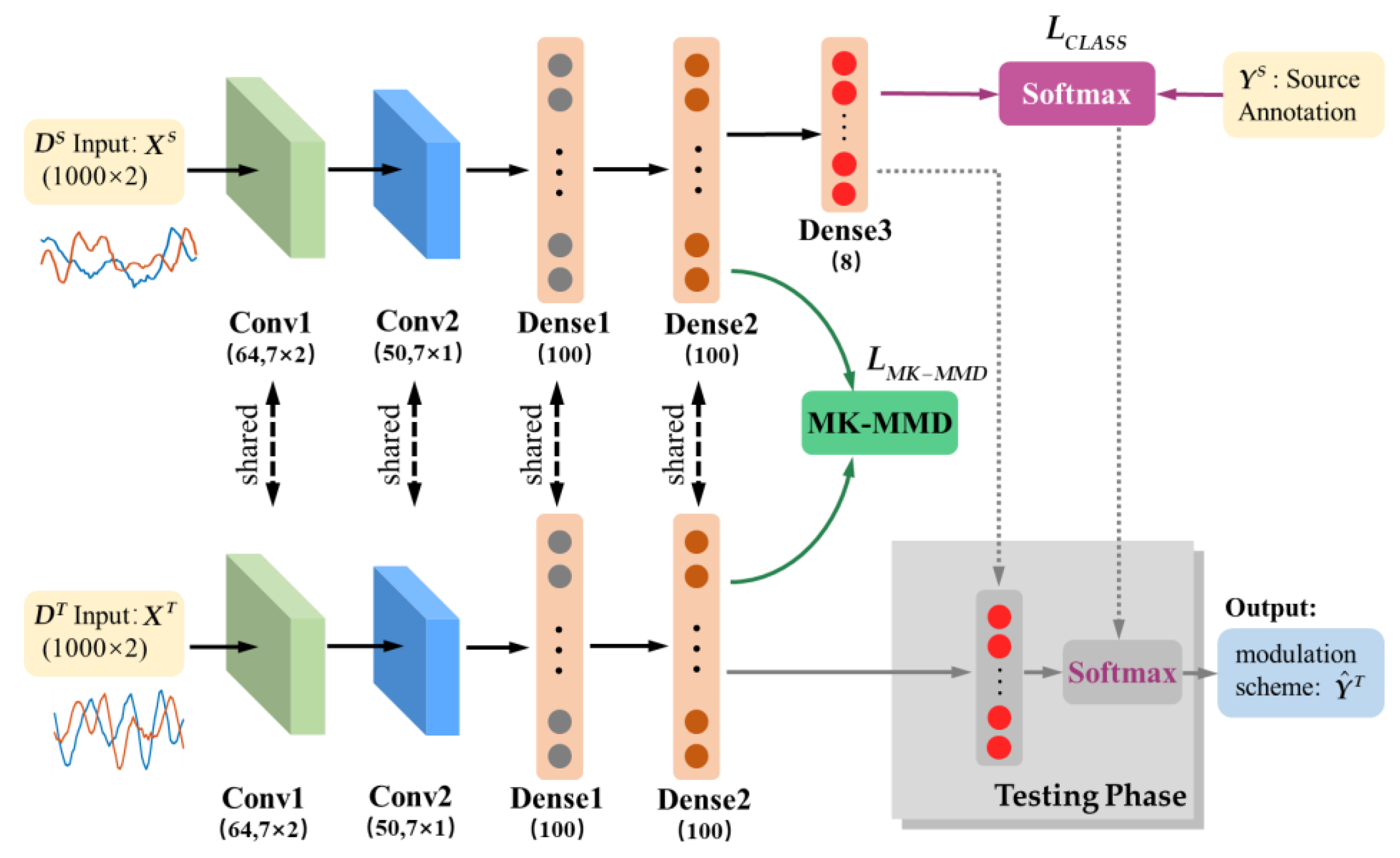
A convolutional neural network (CNN) is a simple yet effective deep structure to exploit the underlying characteristics of different modulation schemes. Considering its wide application in AMC tasks, a four-layer CNN network is adopted as the backbone of the proposed method. Then an adaptation MK-MMD layer is introduced to bridge knowledge from different domains to reduce the dataset bias and the labeling cost. The overall network architecture of the proposed CNN-MK-MMD method is illustrated in Figure 2.
A CNN consisting of two convolutional layers and two dense layers is applied to both well-annotated source data and target data without labels, as shown in Figure 2. Since network weights are shared, there is only one model to be trained in the training phase. Firstly, a ‘Conv1′ convolutional layer consisting of 64 7 × 2 filters is applied to the 1000 × 2 IQ inputs, mapping the time domain inputs into 64 feature channels. Afterward, a ‘Conv2′ convolution layer that has 50 7 × 1 filters are adopted to further enrich the features representation. Then features are fed into the flowing successive cascade of two fully connected dense layers, both consisting of 100 neurons, to learn intrinsic relationships between different modulation schemes. For source domain data with labels Y S , a third dense layer ‘Dense 3′ with N (equals to the number of different modulation schemes in the dataset) neurons is added for supervised learning. Combined with a ‘Softmax’ layer, classification loss L C L A S S could be back propagated to guide weights update.
For target domain unlabeled data, a MK-MMD layer is adopted to improve the robustness against domain discrepancy inspired by [34]. The MK-MMD layer takes the feature map after the ‘Dense2′ layer of both source and target domain as inputs, and thus can measure the distribution differences across domains as discussed in Section 2.2. In this paper, the characteristic kernel of MK-MMD consisted of a family of M Gaussian kernels with varying bandwidth γ that
k m ( X i , X j ) = exp ( X i X j 2 / γ m ) γ m = γ 2 m 1 2 M / / 2 ,   m = 1 , , M
where γ is initialized with the median pairwise distances on the training data and we vary the γ m between 2 2 γ and 2 2 γ with two steps. Based on RKHS distance, MK-MMD loss L M K M M D could be computed. In this way, unlabeled target data are also involved in network training, providing possibilities for a single network with balanced performance on the source and target domains. Note that although we focus our discussion on generalization robustness against different sampling frequencies and symbol rates, there is no such constraints in the application of MK-MMD. It could be easily adapted to other tasks.

3.2. Loss Function and Training Strategy

In the training phase, both source data X S and target data X T are fed into the CNN-MK-MMD network, with different contributions to the loss function. The classification loss is defined as the cross entropy loss to measure the distance between the prediction output y ^ S of the ‘Dense3′ layer and label y S :
L C L A S S = 1 N B i = 1 N B y i log y ^ i S + ( 1 y i S ) log ( 1 y ^ i S )
where N B is the number of training batch size. Target domain un-labeled data involves in network training via MK-MMD loss evaluated by
L M K M M D = d k 2 ( φ ( X D e n s e 2 S ) , φ ( X D e n s e 2 T ) )
which learns the domain discrepancy knowledge based on the feature map of the ‘Dense2′ layer. The final loss function is
L = L C L A S S + λ   L M K M M D
where λ > 0 is a weight parameter balances classification accuracy on the source domain and generalization robustness applied to the target domain.
As depicted in Figure 2, the network is trained collaboratively on source and target datasets for only one time, so that all data flow in a forward way. In the testing phase, ‘Dense2′ features of the target domain samples are fed into the ‘Dense3′ layer inherited from the training procedure (see dashed line in Figure 2). The final output y ^ T is a N × 1 vector indicating its modulation scheme, where N denotes the total number of classes in consideration.

4. Experiments and Result Analysis

To evaluate the effectiveness of the proposed method, a series of experiments are conducted in this section. Firstly, we provide details for the self-established signal datasets and the experimental settings. Next, we investigate the influence of a number of kernels on classification accuracy. Finally, comparison results with state-of-the-art methods are presented.

4.1. Dataset and Experimental Settings

Although there are several authoritative and widely used datasets (e.g., RadioML2016.10a [12,48], RadioML2016.10.b [48], and so on [13] in the AMC field, they do not fit our discussion about the generalization performance across various symbol rates and sampling frequency settings, as the important parameter (number of data samples contained in one modulated symbol, see Equation (3)) is fixed to be eight in all these datasets.
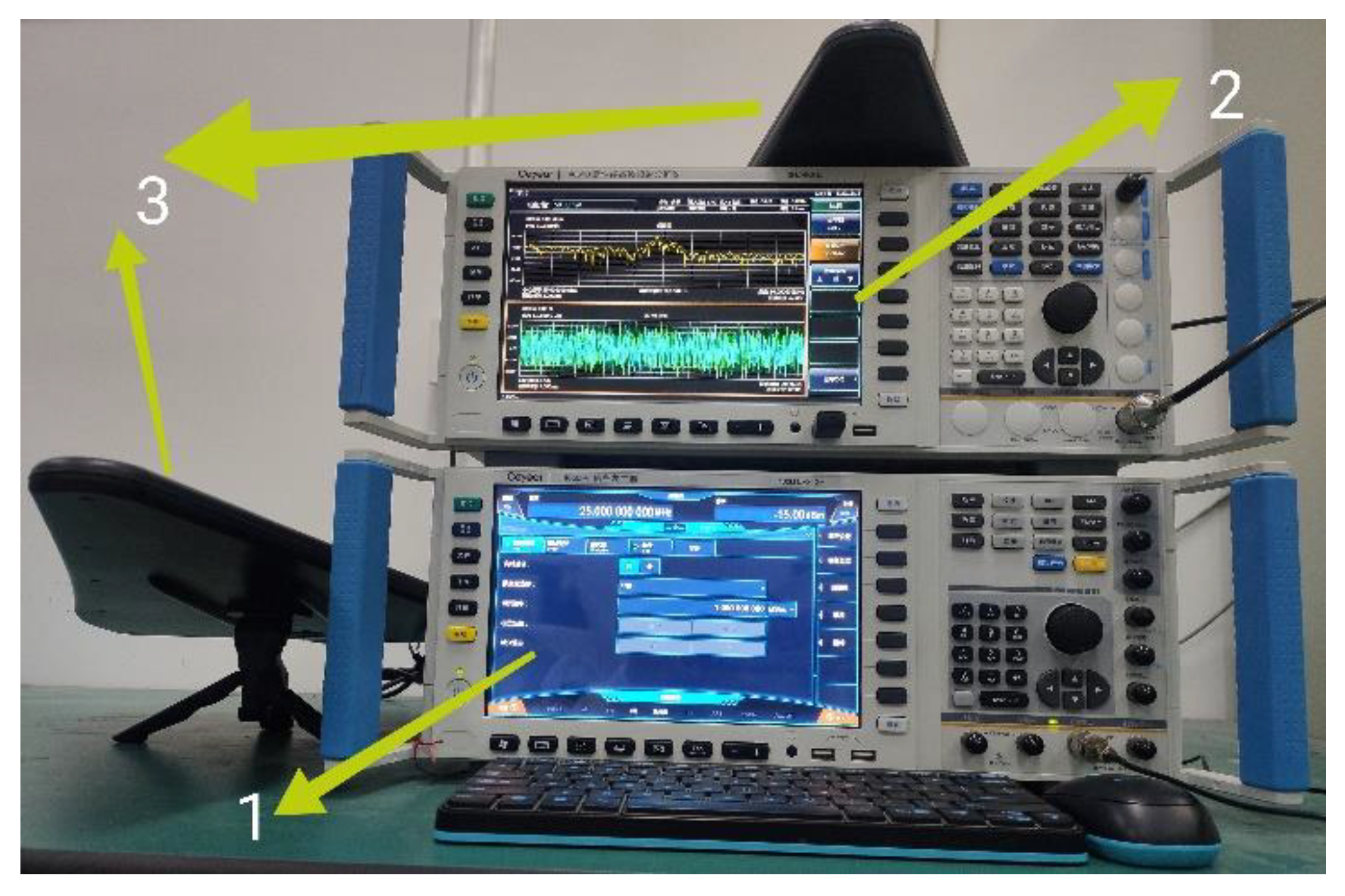
To get rid of this limitation, as well as better simulate real AMC application scenarios, a real-world dataset is constructed with the signal collection system depicted in Figure 3. It consisted of one signal generator, one frequency analyzer, and two antennas with details given in Table 2. Radio signals generated by Ceyear 1465D-V (Ceayer Technologies Co., Ltd., Qingdao, China) are transmitted through sending antenna. All signals are shaped with a root-raised cosine pulse shaping filter with roll-off values set to 0.35. The carrier frequency is set to 10 MHz and the transmission power is −30 dBm. Received signals are uniformly processed by Ceyear 4051B (e.g., high- speed A/D sampling, quadrature down conversion, and so on) before being recorded. Notice that they are about four feet apart without any obstructions between them in a low-noise environment. We segment received samples into a dataset consisting of numerous short-time windows, where in-phase and quadrature (IQ) components of signal samples are recorded to fixed size of 2 × 1000.
Since our main objective is to study the generalization robustness against different combinations of symbol rate R B and sampling frequency F S pairs, we carefully designed three groups of source and target dataset settings as shown in Table 3. Considering the number of sample points per symbol α (defined as FS/RB in Equation (3)) is a key paramter representing certain signal waveform properties, we see our R B - F S settings cover a wide range of α values (varying from 3.125 to 6.25), as compared with state-of-the-art methods [31,33]. Each dataset contains eight digital modulation formats: ASK, BPSK, QPSK, 8PSK, 16PSK, QAM16, QAM32, and QAM64 which are commonly seen in practical applications. For each modulation scheme, 500 signal samples are collected under possible R B - F S pairs in Table 3. Signal samples are then randomly split into training and testing datasets with a ratio of 3:7. Consequently, training and testing dataset sizes in all subsequent experiments are 150 and 350, respectively.
For deep learning hyper-parameters, the batch size is set to NB = 64 to avoid the local minimum and speed up the training process. A dropout rate of dr = 0.5 is adopted to avoid overfitting. The initial learning rate starts at 0.001 and reduces with a multiplicative step of 0.9 for better performance. Stochastic gradient descent (SGD) optimization method updates the weights. All experiments are implemented in PyTorch backend, supported by NVIDIA GeForce GTX TITAN X GPU (NVIDIA, Santa Clara, CA, USA).

4.2. Determination of Number of Kernels

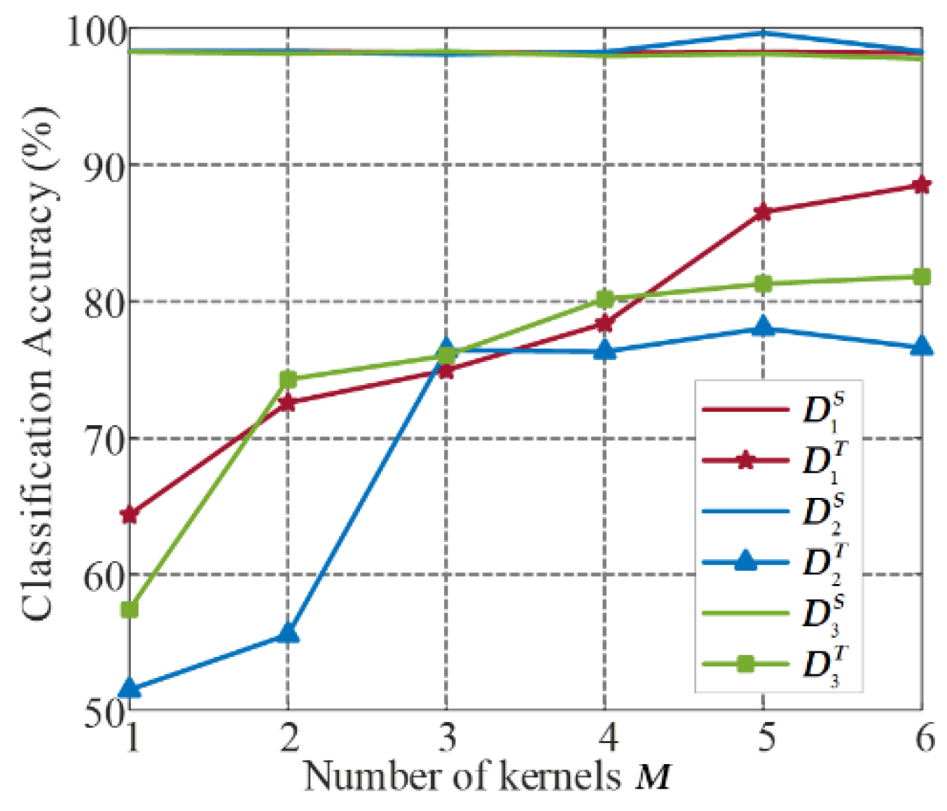
As discussed in Section 2.2, the number of kernels M in MK-MMD plays an important role in characterizing the distribution differences across domains. We start our experiments by exploring the influence of kernel numbers on classification performance.
By varying the number of kernels from 1 to 6, classification accuracy results on both source and target domains are depicted in Figure 4. With well-annotated labels, the proposed MK-MMD method shows similar satisfying classification accuracy (higher than 98%) in all three groups of experiments on the source domain, which maintains relatively stable. For target domain data, and multi-kernels MMD (the number of kernels is larger than one) achieves better performance on the target domain, classification accuracy is above 50% in all cases, and increases with the number of kernels. This could be explained that the relaxation of M do have different bandwidths can better match feature distributions. In this way, the multi-kernel k can mitigate domain discrepancy more effectively as compared with a single-kernel case.
However, monotonic increase in performance stops when M > 5 (tends to be stable on D 3 T in green line, and slightly decline on D 2 T in blue line). Consequently, in comprehensive consideration of overall performance, M is fixed to be 5 in later experiments unless otherwise specified.

4.3. Performance Comparison with State-of-the-Art Methods

To evaluate the effectiveness of the proposed method, comparisons with state-of-the-art methods are conducted, while network properties are summarized in Table 4. For a fair comparison, the two convolutional layers and two dense layers of CNN structure in the proposed method (See Figure 2) are adopted as the benchmark, which is trained on source data only. In CNN-TR [32,33], network weights pre-trained on source data are used to fine-tune a new model on target data where the labels are assumed to be known. Thus there are two separate training procedures and two models trained. In the third comparative work, the spatial transformer network (STN) module [30] is added after CNN, resulting in a slight increase in parameter size and training time. We also replace the MK-MMD layer with CORAL loss [35] in the third dense layer, which is a prevalent statistic in domain adaption to make a comparison. For CORAL and MK-MMD methods, there is no change in parameter size as compared with CNN, only more samples are involved in the statistic calculation. The resulting slight increase in training time cost could be omitted as they can be efficiently computed with linear time approximations.
The classification accuracy comparison of the above methods is summarized in Table 5. All reported results of [30,32,33,35] are based on our re-implementation. For each method, results on both sources and target datasets are given, while the average value is listed in the second line. The figure in bold means the best result among all methods, where the superior performance of the proposed CNN-5K-MMD could be easily observed.
For comparison within the first three fine-tunning based methods, benchmark CNN has poor performance on test data without caring about the domain shifts caused by different symbol rates and sampling frequencies. Conversely, obvious over-fitting occurs in CNN-TR [32,33] and classification accuracy drops dramatically when tested on source data. With the STN module, [30] transforms the input signal for enhanced diversity, and achieved slightly better classification on test data. This suggests that a single network that can simultaneously maintain good performance on both source and target domains is a challenging task.
The three domain adaptation methods, CNN-CORAL, the proposed CNN-1K-MMD, and CNN-5K-MMD take the source and target data in for network training. The resulting performance improvement on the target dataset is remarkable in that average accuracy gain over CNN-STN [30] is 6.32%, 7.88%, and 19.93% on average, verifying the effectiveness of domain adaptation on signal modulation classification. Specifically, CNN-5K-MMD suggests that multiple kernels leverage different kernel bandwidths γ with enhanced robustness. The performance boost demonstrates that CNN-MK-MMD is able to learn transferable features across the different domains.

4.4. Visualizaiton of Confusion Matrix and Feature Distribution

To gain further insights into the classification results among different modulation schemes, the confusion matrix on the source and target datasets is visualized in Figure 5. Results on three datasets are collected for a comprehensive investigation. As compared to the nearly perfect classification in the source dataset, there is still room for improvement in the target domain. Specifically, most classification confusion patterns are within M-PSK and M-QAM modulation groups. For example, 42% of 64QAM signals are misclassified as 16QAM, whereas 36% of 8PSK signals are misclassified as QPSK. Despite their close distances in constellation diagrams, designing a fine-grained domain adaptation network addressing this problem is an important future direction.
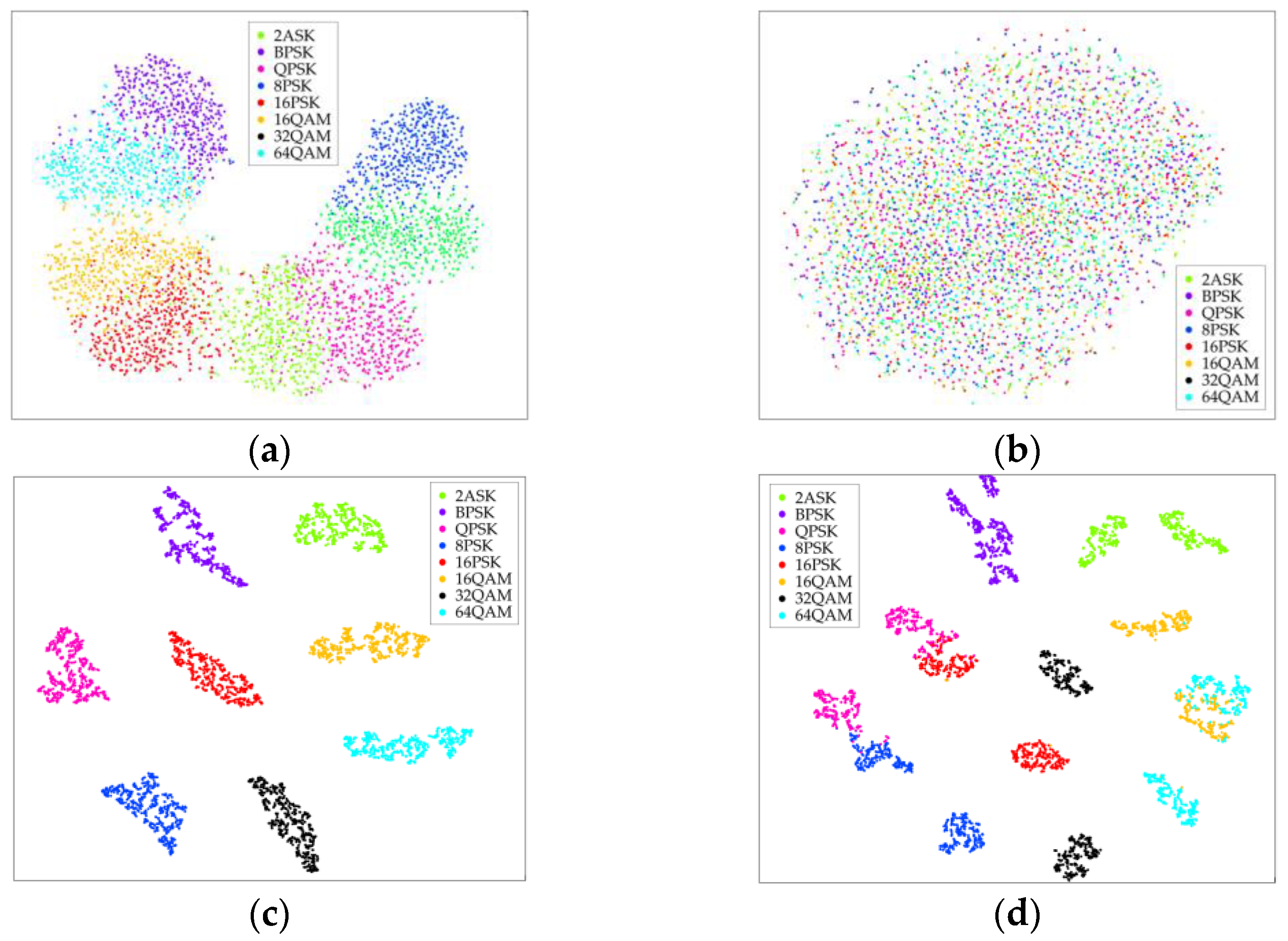
By resorting to the t-SNE [49] method, learned features of CNN and proposed CNN-MK-MMD are visualized in Figure 6. For the CNN network, there is a certain overlap between different modulation schemes on the source dataset (see Figure 6a). However, as shown in Figure 6c, features of different modulation schemes are better discriminated by the proposed CNN-MK-MDD method. This is also in consistent with the nearly perfect classification results in Figure 5.
Since signal distribution under different symbol rates and sampling frequencies are quite different, it is not surprising to observe in Figure 6b that features on target datasets are evenly distributed, which matches the 29.25% accuracy. In sharp contrast to this, one can observe that features in Figure 6d are mostly clustered according to their modulation scheme. However, there are certain misclassifications within the three M-PSK schemes (see pink, red, and blue clusters). This also happens to 16 QAM and 64 QAM. Note that although features of 32 QAM (illustrated in black) are split into two clusters in the test dataset, high accuracy of 95% is achieved. This is a good result for 32 QAM as an in-between modulation scheme. How to design a network that can better exploit underlying distinct features associated with different modulation schemes could be further studied in the future.

5. Conclusions

In this paper, we focus on robust modulation classification of both labeled and unlabeled signals under varying symbol rates and sampling frequency settings. Firstly, the challenge problem is analysed, with the formulation of the parameter α that reflects typical signal shape transformation characteristics. Afterward, a CNN-MK-MMD model is proposed where an MK-MMD layer is imposed to mitigate domain discrepancy of learned CNN features. It is the first-time unsupervised domain adaptation is introduced to alleviate dataset shift caused by signal parameters. Finally, self-build datasets are constructed to verify the effectiveness of the proposed method, which are released for later public use. As compared with state-of-the-art competitors, excellent classification accuracy is reported on both source and unlabeled target datasets under a wide range of α settings. The proposed method provides a new idea for AMC on unlabeled signals, pushing the deep learning deployment toward real practical scenarios.
However, there is still certain confusion within M-PSK and M-QAM modulation schemes, that classification accuracy on target datasets could be further improved. Meanwhile, signal-to-noise ratios (SNR) in the constructed dataset are relatively high as they are collected in an indoor laboratory environment. How to achieve robust classification under complex channel conditions is a promising direction for further study.

Author Contributions

Conceptualization, N.W., Y.L.; methodology, N.W., L.M. and Y.L.; validation, N.W. and Y.Y.; writing—original draft preparation, N.W.; writing—review and editing, Y.L. and H.W. All authors have read and agreed to the published version of the manuscript.

Funding

This research was funded by the National Key R&D Program of China, grant number 2018YFF01014304, and the Shandong Provincial Natural Science Foundation of China, grant numbers ZR2019ZD01,ZR2020MF027, ZR2020MF143 and ZR2021QF141.

Data Availability Statement

The data used in the paper are open and available on the website: https://pan.baidu.com/s/1rvdgxPa90ipgPdqlSTUpdQ and the Key:2022 (accessed on 10 November 2022).

Conflicts of Interest

The authors declare no conflict of interest.

References

  1. Dobre, O.A.; Abdi, A.; Bar-Ness, Y.; Su, W. Survey of automatic modulation classification techniques: Classical approaches and new trends. IET Commun. 2007, 1, 137–156. [Google Scholar] [CrossRef] [Green Version]
  2. Huang, S.; Yao, Y.; Wei, Z.; Feng, Z.; Zhang, P. Automatic modulation classification of overlapped sources using multiple cumulants. IEEE Trans. Veh. Technol. 2017, 66, 6089–6101. [Google Scholar] [CrossRef]
  3. Han, L.; Gao, F.; Li, Z.; Dobre, O.A. Low complexity automatic modulation classification based on order-statistics. IEEE Trans. Wirel. Commun. 2017, 16, 400–411. [Google Scholar] [CrossRef]
  4. Jafar, N.; Paeiz, A.; Farzaneh, A. Automatic modulation classification using modulation fingerprint extraction. J. Syst. Eng. Electron. 2021, 32, 799–810. [Google Scholar] [CrossRef]
  5. Wu, H.; Hua, X. A review of digital signal modulation methods based on wavelet transform. In Proceedings of the 2020 IEEE International Conference on Mechatronics and Automation (ICMA), Beijing, China, 13–16 October 2020; pp. 1123–1128. [Google Scholar] [CrossRef]
  6. He, K.; Zhang, X.; Ren, S.; Sun, J. Deep residual learning for image recognition. In Proceedings of the 2016 IEEE Conference on Computer Vision and Pattern Recognition (CVPR), Las Vegas, NV, USA, 27–30 June 2016; pp. 770–778. [Google Scholar] [CrossRef] [Green Version]
  7. Eliasmith, Y.T.C. Deep networks for robust visual recognition. In Proceedings of the 27th International Conference on International Conference on Machine Learning, Omnipress, Haifa, Israel, 21–24 June 2010; pp. 1055–1062. [Google Scholar]
  8. Voulodimos, A.; Doulamis, N.; Doulamis, A.; Protopapadakis, E. Deep learning for computer vision: A brief review. Comput. Intell. Neurosci. 2018, 2018, 7068349. [Google Scholar] [CrossRef]
  9. Hinton, G.; Deng, L.; Yu, D.; Dahl, G.; Mohamed, A.-R.; Jaitly, N.; Senior, A.; Vanhoucke, V.; Nguyen, P.; Sainath, T.; et al. Deep neural networks for acoustic modeling in speech recognition: The shared views of four research groups. IEEE Signal Process. Mag. 2012, 29, 82–97. [Google Scholar] [CrossRef]
  10. Dahl, G.E.; Dong, Y.; Li, D.; Acero, A. Context-dependent pre-trained deep neural networks for large-vocabulary speech recognition. IEEE Trans. Audio Speech Lang. Process. 2012, 20, 30–42. [Google Scholar] [CrossRef] [Green Version]
  11. Young, T.; Hazarika, D.; Poria, S.; Cambria, E. Recent trends in deep learning based natural language processing [Review Article]. IEEE Comput. Intell. Mag. 2018, 13, 55–75. [Google Scholar] [CrossRef]
  12. O’Shea, T.J.; Corgan, J.; Clancy, T.C. Convolutional radio modulation recognition networks. Comm. Com. Inf. Sci. 2016, 629, 213–226. [Google Scholar] [CrossRef] [Green Version]
  13. O’Shea, T.J.; Roy, T.; Clancy, T.C. Over-the-air deep learning based radio signal classification. IEEE J. Sel. Top. Signal Process. 2018, 12, 168–179. [Google Scholar] [CrossRef] [Green Version]
  14. Zhang, Z.; Luo, H.; Wang, C.; Gan, C.; Xiang, Y. Automatic modulation classification using CNN-LSTM Based dual-stream structure. IEEE Trans. Veh. Technol. 2020, 69, 13521–13531. [Google Scholar] [CrossRef]
  15. Zhang, F.; Luo, C.; Xu, J.; Luo, Y.; Zheng, F.-C. Deep learning based automatic modulation recognition: Models, datasets, and challenges. Digit. Signal Process. 2022, 129, 103650. [Google Scholar] [CrossRef]
  16. Zhou, R.; Liu, F.; Gravelle, C.W. Deep learning for modulation recognition: A survey with a demonstration. IEEE Access 2020, 8, 67366–67376. [Google Scholar] [CrossRef]
  17. Liu, Y.; Liu, Y.; Yang, C. Modulation recognition with graph convolutional network. IEEE Wirel. Commun. Lett. 2020, 9, 624–627. [Google Scholar] [CrossRef]
  18. Krzyston, J.; Bhattacharjea, R.; Stark, A. Complex-valued convolutions for modulation recognition using deep learning. In Proceedings of the 2020 IEEE International Conference on Communications Workshops (ICC Workshops), Dublin, Ireland, 7–11 June 2020; pp. 1–6. [Google Scholar] [CrossRef]
  19. Zeng, Y.; Zhang, M.; Han, F.; Gong, Y.; Zhang, J. Spectrum analysis and convolutional neural network for automatic modulation recognition. IEEE Wirel. Commun. Lett. 2019, 8, 929–932. [Google Scholar] [CrossRef]
  20. Peng, S.; Jiang, H.; Wang, H.; Alwageed, H.; Zhou, Y.; Sebdani, M.M.; Yao, Y.D. Modulation classification based on signal constellation diagrams and deep learning. IEEE Trans. Neural. Netw. Learn. Syst. 2019, 30, 718–727. [Google Scholar] [CrossRef] [PubMed]
  21. Huang, S.; Jiang, Y.; Gao, Y.; Feng, Z.; Zhang, P. Automatic modulation classification using contrastive fully convolutional network. IEEE Wirel. Commun. Lett. 2019, 8, 1044–1047. [Google Scholar] [CrossRef]
  22. Kumar, Y.; Sheoran, M.; Jajoo, G.; Yadav, S.K. Automatic modulation classification based on constellation density using deep learning. IEEE Commun. Lett. 2020, 24, 1275–1278. [Google Scholar] [CrossRef]
  23. Liu, M.; Liao, G.; Zhao, N.; Song, H.; Gong, F. Data-Driven deep learning for signal classification in industrial cognitive radio networks. IEEE Trans. Ind. Inform. 2021, 17, 3412–3421. [Google Scholar] [CrossRef]
  24. Zhang, M.; Zeng, Y.; Han, Z.D.; Gong, Y. Automatic modulation recognition using deep learning architectures. IEEE Int. Work. Sign. P 2018, 281–285. [Google Scholar] [CrossRef]
  25. Wang, Y.; Liu, M.; Yang, J.; Gui, G. Data-driven deep learning for automatic modulation recognition in cognitive radios. IEEE Trans. Veh. Technol. 2019, 68, 4074–4077. [Google Scholar] [CrossRef]
  26. O’Shea, N.E.W.T.J. Deep architectures for modulation recognition. In Proceedings of the 2017 IEEE International Symposium on Dynamic Spectrum Access Networks (DySPAN), Baltimore, MD, USA, 6–9 March 2017; pp. 1–6. [Google Scholar] [CrossRef] [Green Version]
  27. Ghasemzadeh, P.; Hempel, M.; Sharif, H. GS-QRNN: A high-efficiency automatic modulation classifier for cognitive radio IoT. IEEE Internet Things J. 2022, 9, 9467–9477. [Google Scholar] [CrossRef]
  28. Ghasemzadeh, P.; Banerjee, S.; Hempel, M.; Sharif, H. A novel deep learning and polar transformation framework for an adaptive automatic modulation classification. IEEE Trans. Veh. Technol. 2020, 69, 13243–13258. [Google Scholar] [CrossRef]
  29. Chang, S.; Huang, S.; Zhang, R.; Feng, Z.; Liu, L. Multitask-learning-based deep neural network for automatic modulation classification. IEEE Internet Things J. 2022, 9, 2192–2206. [Google Scholar] [CrossRef]
  30. Perenda, E.; Rajendran, S.; Bovet, G.; Pollin, S.; Zheleva, M. Learning the unknown: Improving modulation classification performance in unseen scenarios. In Proceedings of the IEEE Conference on Computer Communications, Vancouver, BC, Canada, 10–13 May 2021. [Google Scholar] [CrossRef]
  31. Bu, K.; He, Y.; Jing, X.; Han, J. Adversarial transfer learning for deep learning based automatic modulation classification. IEEE Signal Process. Lett. 2020, 27, 880–884. [Google Scholar] [CrossRef]
  32. Wang, Q.; Du, P.; Yang, J.; Wang, G.; Lei, J.; Hou, C. Transferred deep learning based waveform recognition for cognitive passive radar. Signal Process. 2019, 155, 259–267. [Google Scholar] [CrossRef]
  33. Xu, Y.; Li, D.; Wang, Z.; Guo, Q.; Xiang, W. A deep learning method based on convolutional neural network for automatic modulation classification of wireless signals. Wirel. Netw. 2018, 25, 3735–3746. [Google Scholar] [CrossRef]
  34. Long, M.S.; Cao, Y.; Wang, J.M.; Jordan, M.I. Learning transferable features with deep adaptation networks. Pr. Mach. Learn. Res. 2015, 37, 97–105. [Google Scholar]
  35. Sun, B.C.; Saenko, K. Deep CORAL: Correlation alignment for deep domain adaptation. Lect. Notes Comput. Sci. 2016, 9915, 443–450. [Google Scholar] [CrossRef] [Green Version]
  36. Inoue, N.; Furuta, R.; Yamasaki, T.; Aizawa, K. Cross-domain weakly-supervised object detection through progressive domain adaptation. In Proceedings of the 2018 IEEE/CVF Conference on Computer Vision and Pattern Recognition, Salt Lake City, UT, USA, 18–23 June 2018; pp. 5001–5009. [Google Scholar] [CrossRef] [Green Version]
  37. Tang, Y.; Wang, J.; Gao, B.; Dellandrea, E.; Gaizauskas, R.; Chen, L. Large Scale Semi-Supervised Object Detection Using Visual and Semantic Knowledge Transfer. In Proceedings of the 2016 IEEE Conference on Computer Vision and Pattern Recognition (CVPR), Las Vegas, NV, USA, 27–30 June 2016; pp. 2119–2128. [Google Scholar] [CrossRef] [Green Version]
  38. Zhang, J.; Li, W.; Ogunbona, P. Joint geometrical and statistical alignment for visual domain adaptation. In Proceedings of the 2017 IEEE Conference on Computer Vision and Pattern Recognition (CVPR), Honolulu, HI, USA, 21–26 July 2017; pp. 5150–5158. [Google Scholar] [CrossRef] [Green Version]
  39. Tzeng, E.; Hoffman, J.; Saenko, K.; Darrell, T. Adversarial discriminative domain adaptation. In Proceedings of the 2017 IEEE Conference on Computer Vision and Pattern Recognition (CVPR), Honolulu, HI, USA, 21–26 July 2017; pp. 2962–2971. [Google Scholar] [CrossRef] [Green Version]
  40. Han, Z.; Gui, X.J.; Sun, H.; Yin, Y.; Li, S. Towards accurate and robust domain adaptation under multiple noisy environments. IEEE Trans. Pattern Anal. Mach. Intell. 2022, 1–18. [Google Scholar] [CrossRef]
  41. Gallego, A.J.; Calvo-Zaragoza, J.; Fisher, R.B. Incremental unsupervised domain-adversarial training of neural networks. IEEE Trans. Neural Netw. Learn. Syst. 2021, 32, 4864–4878. [Google Scholar] [CrossRef] [PubMed]
  42. Zhu, Y.; Zhuang, F.; Wang, J.; Ke, G.; Chen, J.; Bian, J.; Xiong, H.; He, Q. Deep subdomain adaptation network for image classification. IEEE Trans. Neural Netw. Learn. Syst. 2021, 32, 1713–1722. [Google Scholar] [CrossRef] [PubMed]
  43. Wang, M.; Deng, W. Deep visual domain adaptation: A survey. Neurocomputing 2018, 312, 135–153. [Google Scholar] [CrossRef] [Green Version]
  44. Patel, V.M.; Gopalan, R.; Li, R.; Chellappa, R. Visual domain adaptation: A survey of recent advances. IEEE Signal Process. Mag. 2015, 32, 53–69. [Google Scholar] [CrossRef]
  45. Borgwardt, K.M.; Gretton, A.; Rasch, M.J.; Kriegel, H.P.; Scholkopf, B.; Smola, A.J. Integrating structured biological data by Kernel maximum mean discrepancy. Bioinformatics 2006, 22, e49–e57. [Google Scholar] [CrossRef] [PubMed] [Green Version]
  46. Sun, B.; Feng, J.; Saenko, K.J. Return of frustratingly easy domain adaptation. arXiv 2015, arXiv:1511.05547. [Google Scholar] [CrossRef]
  47. Long, M.; Zhu, H.; Wang, J.; Jordan, M.I.J. Deep transfer learning with joint adaptation networks. arXiv 2016, arXiv:1605.06636. [Google Scholar]
  48. O’Shea, T.J.; West, N. Radio machine learning dataset generation with GNU radio. In Proceedings of the GNU Radio Conference, Boulder, CO, USA, 12–16 September 2016. [Google Scholar]
  49. Maaten, L.J.P.; Hinton, G.E. Visualizing high-dimensional data using t-sne. J. Mach. Learn. Res. 2008, 9, 2579–2605. [Google Scholar]
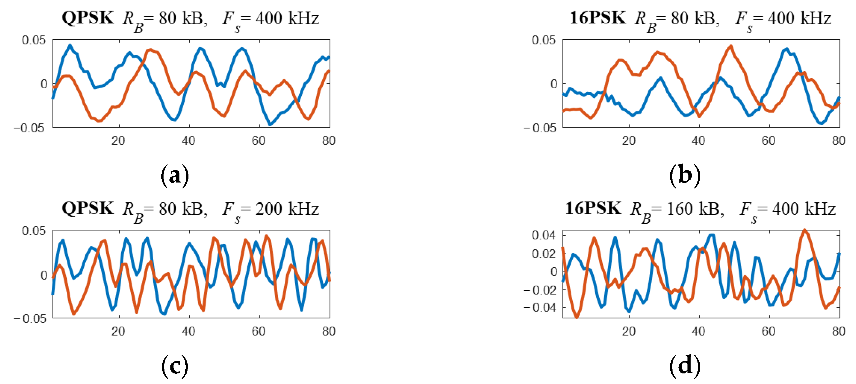
Figure 1. Signal examples with varying symbol rates ( R B ) at different sampling frequencies ( F s ). Red line represents I conponents and blue line represents Q components. (a) QPSK signal, whose RB is 80k baud and FS is 400kHz; (b) 16PSK signal, whose RB is 80k baud and FS is 400kHz; (c) QPSK signal, whose RB is 80k baud and FS is 200kHz; and (d) 16PSK signal, whose RB is 160k baud and FS is 400kHz.
Electronics 12 00066 g001
Figure 2. Illustration of the proposed CNN-MK-MMD architecture.
Electronics 12 00066 g002
Figure 3. Configuration for signal collection system. (In the paper, we use Table 2 to explain for the number 1-3. ”1“ is signal genertor Ceyear 1465D-V; 2 is frequency analyzer Ceyear 4051B; “3” is antennas HyperLOG3080X. It consisted of one signal generator, one frequency analyzer, and two antennas with details given in Table 2”).
Electronics 12 00066 g003
Figure 4. Classification accuracy comparison over different number of kernels.
Electronics 12 00066 g004
Figure 5. Confusion matrices of CNN-MK-MDD on (a) source and (b) target datasets.
Electronics 12 00066 g005
Figure 6. Feature visualization by t-SNE of CNN features on (a) source and (b) target datasets, and CNN-MK-MMD features on (c) source and (d) target datasets.
Electronics 12 00066 g006
Table 1. Different transfer learning methods in AMC.
MethodsModelDataset TypeVariation Setting
(DSDT)
No. of ModelsImproved Domain
Feature ExtractionRN [13]BothSynthetic—Real2Target
STN-ResNeXt [30]SyntheticFs:1.5k—1k and 2k1Both
Fine-TuningATLA [31]SyntheticFs:Fs—1/2 Fs2Target
TCNN-BL [32]SyntheticFs:1M—0.5M2Target
CNNs-TR [33]RealSNR Variation2Target
Table 2. Devices used in signal collection system.
NumberDevice NamesModel Number
1signal generatorCeyear 1465D-V (Ceayer Technologies Co., Ltd., Qingdao, China)
2frequency analyzerCeyear 4051B(Ceayer Technologies Co., Ltd., Qingdao, China)
3antennaHyperLOG3080X(HyperLOG3080X is AARONIA, Germany)
Table 3. Symbol rate and sampling frequency settings of different source and target datasets.
DatasetSymbol Rate RB (Baud)Sampling Frequency
FS (Hz)
No. Points per Symbol α (FS/RB)
Source dataset 1 ( D 1 S )80k400k6.250
Target dataset 1 ( D 1 T )120k400k4.167
Source dataset 2 ( D 2 S )120k400k4.167
Target dataset 2 ( D 2 T )160k400k3.125
Source dataset 3 ( D 3 S )80k400k6.250
Target dataset 3 ( D 3 T )80k200k3.125
Table 4. State-of-the-art AMC method in comparison.
MethodsTarget Label NeededNo. of
Models
Parameter
(MB)
Trainning Time (Epoch/s)
CNNN18.731.628
CNN-TR [32,33]Y28.731.625
CNN-STN [30]N110.111.731
CNN-CORAL [35]N18.731.639
CNN-1K-MMDN18.731.653
CNN-5K-MMDN18.731.659
Table 5. Classification Accuracy comparison with state-of-the-art methods.
Methods D 1 S D 1 T D 2 S D 2 T D 3 S D 3 T Average
CNN99.20%29.69%97.64%36.82%97.50%21.25%63.68%
64.45%67.23%59.38%
CNN-TR [32,33]15.70%96.71%23.26%78.50%21.25%79.79%52.54%
56.21%50.88%50.52%
CNN-STN [30]97.62%45.38%90.50%46.38%98.25%41.00%69.86%
71.50%68.44%69.63%
CNN-CORAL [35]98.29%70.54%87.39%50.32%98.29%52.25%76.18%
84.42%68.86%75.27%
CNN-1K-MMD98.25%64.29%98.29%51.29%98.25%57.25%77.94%
81.27%74.79%77.75%
CNN-5K-MMD98.25%86.61%98.21%77.36%98.21%80.11%89.79%
92.43%87.79%89.16%
Disclaimer/Publisher’s Note: The statements, opinions and data contained in all publications are solely those of the individual author(s) and contributor(s) and not of MDPI and/or the editor(s). MDPI and/or the editor(s) disclaim responsibility for any injury to people or property resulting from any ideas, methods, instructions or products referred to in the content.