Voltage Based Electronic Control Unit (ECU) Identification with Convolutional Neural Networks and Walsh–Hadamard Transform

Abstract

This paper proposes an identification approach for the Electronic Control Units (ECUs) in the vehicle, which are based on the physical characteristics of the ECUs extracted from their voltage output. Then, the identification is not based on cryptographic means, but it could be used as an alternative or complementary means to strengthen cryptographic solutions for vehicle cybersecurity. While previous research has used hand-crafted features such as mean voltage, max voltage, skew or variance, this study applies Convolutional Neural Networks (CNNs) in combination with the Walsh–Hadamard Transform (WHT), which has useful properties of compactness and robustness to noise. These properties are exploited by the CNN, and in particular, the pooling layers, to reduce the size of the feature maps in the CNN. The proposed approach is applied to a recently public data set of ECU voltage fingerprints extracted from different automotive vehicles. The results show that the combination of CNN and the WHT outperforms, in terms of identification accuracy, robustness to noise and computing times, and other approaches proposed in the literature based on shallow machine learning and tailor-made features, as well as CNN with other linear transforms such as the Discrete Fourier Transform (DFT) or CNN with the original time domain representations.

1. Introduction

Vehicular cybersecurity has received increased attention by the research community in recent years due to a number of factors. One of the factors is the connectivity of vehicles, which can provide an interface to attackers, as demonstrated by the taking over of a Jeep through a remote connection by Miller and Valasek, and documented in [1]. Another factor is related to the implementation of sophisticated functions in modern vehicles to improve automation. These functions are implemented with software modules hosted in Electronic Control Units (ECUs), which are connected through the internal in-vehicle network among themselves and with the sensors in the vehicle [2]. An extensive survey on potential cybersecurity attacks on modern vehicles is provided in [3]. Several countermeasures have been designed by the research community to address the different attacks. A potential masquerading attack is the installation of a malicious ECU to replace a legitimate ECU with the objective of collecting data from the vehicle or injecting false messages into the in-vehicle network to hamper the functioning of the vehicle. Masquerading attacks can be prevented by a number of authentication techniques. The conventional authentication technique is based on cryptographic means, but it requires the secure storing of keys in the ECU, which can be cumbersome and costly. In addition, cryptographic authentication raises backward compatibility issues and requires demanding key management procedures in the automotive sector; moreover, accommodating cryptographic material in the limited 64-bit payload of CAN frames is in itself challenging. Consequently, much more work is needed before CAN networks can fully support cryptographic algorithms. Another authentication technique recently proposed in the communication domain is based on the intrinsic physical features of electronic devices. The concept is that small differences in the design and implementation of electronic devices (e.g., ECUs) can be used to identify and distinguish them, even if they support the same communication standard (e.g., CAN-bus in the automotive domain). This technique has its own limitations, as discussed in the rest of this paper, but it also has the benefit in that there is no need to protect the cryptographic material as it is already embedded in the design and implementation of the ECU itself. It is also relatively easy to implement. The identification of the ECUs using this technique can be based on statistical methods (e.g., the variance of the signal output by the ECU) or machine learning methods based on hand-crafted features (e.g., the average power level or the entropy of the signal output of the ECU). In recent years, Deep Learning (DL) has been applied to this form of authentication, with significant improvements in performance identification and without the need to design hand-crafted features [4].

This study proposes the application of the Walsh–Hadamard transform in combination with CNN to the problem of ECU identification in in-vehicle networks. The Walsh–Hadamard transform has been used with success in a number of domains (including the field of security) because of a number of advantages in comparison to other transforms: it provides a compressed representation of the main components of a signal (as shown in the rest of this paper), it has N(Log N) algorithm complexity in its fast Walsh–Hadamard implementation, and it performs a real to real transform (which is useful for the real voltage output of the ECU). The results furnished in this paper show that the Walsh–Hadamard transform combined with CNN is particularly suited for the identification of ECUs and it significantly outperforms other approaches from the literature using CNNs. The proposed approach is evaluated on the recently published ECUPrint data set [5], which is a recent (2022) and extensive data set of voltage signals collected by more than 40 ECUs.

2. Related Work

The exploitation of the physical fingerprints of ECU devices in the in-vehicle networks was the subject of a number of recent papers, which are reviewed in this section. It is noted that this form of identification and authentication has been used for a number of years in other contexts and for other types of electronic device. For example, the recent survey [6] describes the application of this technique for wireless devices. This survey and other studies [7] have shown that the application of Deep Learning significantly improves classification accuracy compared to shallow machine learning approaches at the cost of increased computing complexity and time. In the automotive sector, few studies have applied machine learning and Deep Learning to the fingerprints of automotive components, including the ECUs and the sensors present in a vehicle. Two main categories of ECU identification based on physical fingerprints can be defined: The first category is based on the use of the ECU clock skew, which is related to the consideration that each ECU on the CAN bus has a different hardware clock, which has a different clock speed due to variations in the clock’s hardware crystal. Some examples of studies in this category are [8,9,10]. The second category is more general, and it exploits the signal in the time domain without the clock skew information. A limitation of the approaches based on the first category is that an attacker can easily reproduce the clock skew. Moreover, these approaches may not work for on-event transmissions, and are affected by processing and arbitration delays [5]. The approaches based on the second category use many other characteristics of the signal (e.g., shape and frequency response), which are much more difficult to reproduce. For this reason, this study does not use a skew approach, and the data of the voltage outputs are synchronized and normalized to remove the skew information. This may also make the data set more challenging for classification. In the second category, some of the first papers to use time- and frequency-based features extracted from the voltage output of an ECU were [11,12] where the classification of electrical CAN signals using a support vector machine (SVM), a neural network (NN), and a bagged decision tree (BDT) was investigated. In [13] a similar approach is applied based on the application of statistical features such as mean, standard deviation, variance, and skewness to the ECU voltage signal are applied in [13].

The problem is that hand-crafted features (e.g., variance) must be selected, which may not be optimal in the wide feature space. Then, more recent papers have proposed to use Deep Learning algorithms like in [14], where the authors have used Recurrent Neural Networks with Long Short-Term Memory to classify CAN data frame senders (e.g., ECUs) based on the analog voltage signal characteristics of each frame, which are uniquely identifiable from unique analog wire responses and ECU transceiver fingerprints. Another example of the application of Deep Learning algorithms, and more specifically, CNN, which was also used in this study, is [4], where CNN is applied directly to the voltage signals transmitted by the ECU transceivers on the in-vehicle network. Contrary to [4], this paper also attempts other spectral representations of the voltage signal (in particular, the WHT), demonstrating a superior classification performance to the original time domain representation.

We complete this review of the literature by mentioning studies in other domains (not related to the automotive sector) where WHT was applied together with CNN for classification purposes. In [15], the authors have applied the combination of WHT with CNN in the forest fire response for the detection of embers, also called firebrands, which can act as wildfire super-spreaders. The authors exploit the compactness of WHT representation from images/video to improve the efficiency and accuracy of the ember detection. In [16], the authors have applied WHT in combination with CNN to address the issue of sensitivity drift compensation for chemical sensors. The use of WHT is compared with Discrete Cosine Transform (DCT), and the results show that the approach based on WHT provides a higher accuracy performance.

In summary, the studies on the application of DL to ECU identification based on their physical features are quite rare, and no study has used WHT for this problem. On the other hand, some studies in other domains have shown the superior performance of WHT to other transforms for classification purposes. Then, this paper aims to address this gap for ECU identification.

The structure of this paper is the following. Section 2 reviews the related work on ECU identification from its voltage output using machine learning or Deep Learning methods. Section 3 describes the overall workflow of the proposed approach, the description of the ECUPrint data set used in this study, and the SAE J1939 standard, in particular for the physical layer. Section 4 describes the transforms used in this paper: the Fast Fourier Transform, the Discrete Hartley Transform, and the Walsh–Hadamard transform, with a specific focus on the latter. Section 5 describes the CNN architecture, its hyperparameters, and the other machine learning algorithms used in this study, together with the metrics of evaluation and the computing platform. The results are presented and discussed in Section 6, where a comparison with the approaches from the literature is also provided. Finally, Section 7 concludes this paper and points out future developments.

3. Methodology and Materials

This section describes the methodology used to implement the approach proposed in this study, and the data set used to evaluate it. A brief description of the in-vehicle network standard used in this study is presented in Section 3.1. Then, the overall workflow and the data set are presented in the subsequent subsections.

3.1. SAE J1939 and ISO 11898

This section is used to describe the SAE J1939 standard [17], which is the main in-vehicle standard in the automotive sector. SAE J1939 is based on five layers in the seven-layer OSI network model, including the Controller Area Network (CAN) ISO 11898 specification (with the 29-bit extended identifier) for the physical and data-link layers [18].

The CAN network is designed to be robust and resilient to potential disturbances in the vehicle due to magnetic fields, vibration, thermal excursions, and aging [19]. The CAN network is the in-vehicle network in the automotive vehicle, which allows the ECUs and sensors (e.g., powertrain sensors) to exchange data with a baudrate of up to 1 Mbps (in ISO 11898) using a twisted two-wire cable. The standard is defined to use differential wired-AND signals: CAN high (CANH) and CAN low (CANL). The dominant state is represented by CANH > CANL in voltage values, and the recessive state is represented by CANH ≤ CANL. A 0 data bit encodes a dominant state, while a 1 data bit encodes a recessive state, supporting a wired-AND convention, which gives nodes with lower ID numbers priority on the bus. For example, a dominant bit is transmitted when CANL is around 1.5 V and CANH is around 3.5 V [18].

Data are transmitted in CAN-frames with an 11 bit arbitration field in the base frame format and a 29 bit arbitration field in the Extended frame format. The data payload is made up of 8 bytes. Other fields in the CAN frame are associated with the CRC and control bits [17]. Because the study only exploits the physical layer of the protocol, the rest of the design of SAE J1939 and ISO 11898 is not described here. Because CANH and CANL are represented with the terms Voltage A and Voltage B in the reference data set [5], these terms will be used in the remainder of this article.

3.2. Workflow

The overall workflow of the proposed approach is proposed in Figure 1, and each step is described in the following bullet list.

• In the first step, the ECU data set (described in detail in Section 3.3) is processed to combine the signals of Voltage A and Voltage B, as the approach proposed in this study is based on both signals. As shown later, in the Results Section 6, a comparison with a data set composed only of Voltage A or Voltage B is also executed, but the results show that the combination of the two signals, Voltage A and B, provides a higher identification performance.
• The signals are synchronized and normalized to ensure that the approach is uniquely based on the shape of the signals and not on other factors such as the difference in timing (e.g., based on the evaluation of the skew). In this way, the proposed approach is robust against spoofing attacks based on timing/skew.
• To emulate the presence of noise in the vehicle environment, and in particular, in the in-vehicle network where the ECU is connected, AWGN is added to the signals in the data set to emulate different SNR conditions. The ’awgn’ MATLAB function from the signal processing toolbox is used for this purpose.
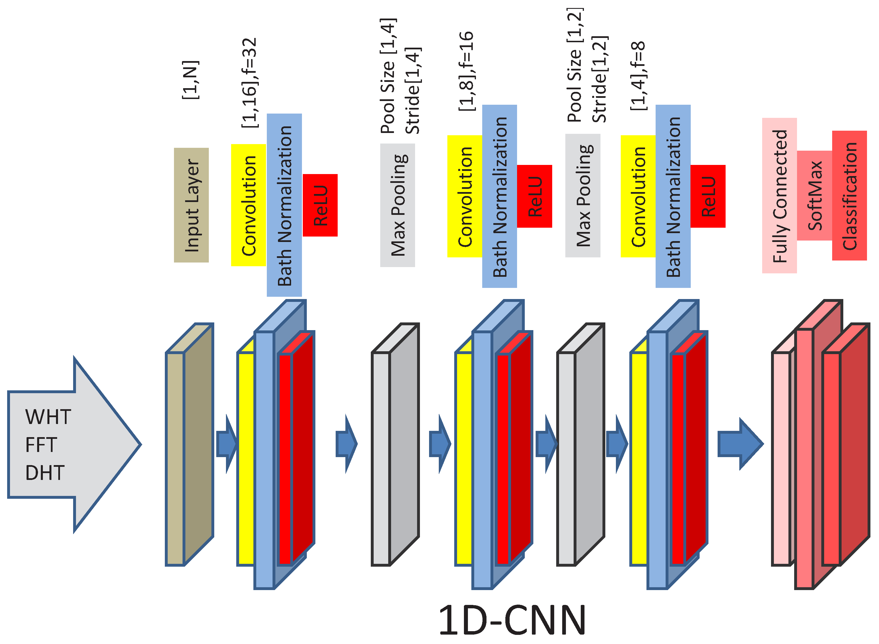
• The combination of Voltage A and Voltage B signals with the added noise are submitted to different transforms. In particular, these are WHT, FFT, and DHT. To make the comparison consistent (since both WHT and DHT provide a real value), only the amplitude component of FFT is used in the analysis. Further results not presented in this paper for space reasons show that the identification accuracy with only the amplitude component of the FFT significantly outperforms both the phase component of the FFT and the combination of the amplitude and phase components. For this reason, only the amplitude of FFT is used in the rest of this study. The FFT is used because it is a common choice in the literature for physical layer authentication [6,20]. DHT was chosen because it is another Fourier-related transform that transforms a real signal to a real signal like WHT. In addition, it has been used with success [21] for sensor physical layer authentication based on voltage signals in the automotive sector. All of these transforms are implemented and executed in parallel (as shown in Figure 1).
  In addition, for the original time domain signal, statistical features are applied to generate a feature space for classification. A feature-based approach was also used on the same data set in [5], and it is also common in physical layer authentication [20]. This paper has used the following statistical features: mean, variance, skewness, kurtosis, Shannon entropy, and maximum value, which are chosen because they are related to features already used in the literature for physical layer identification [5,13,20], and because of their efficient computation. The statistical features are applied to the Voltage A and Voltage B signals.
• CNN was used to process the output of WHT, FFT (amplitude), DHT, and the original time representation. Instead, machine learning algorithms (i.e., Decision Tree and K-Nearest Neighbor) were used for the feature-based approach and for a subset of WHT when it is significantly reduced.

An algorithmic description of the workflow is provided in Algorithm 1.

3.3. Electronic Control Unit Data Set

The ECUprint data set described in [5] is used in this study with slight modifications (described in the rest of this section) from the original data set. The ECUPrint data set is a collection of raw CAN voltage samples and CAN logs collected from 10 vehicles, ranging from small cars to SUVs and a heavy-duty vehicle, totaling 54 ECUs. The Pico Scope 5000 Series was used to collect the voltage signals. The sample rate used to collect the voltage signals (e.g., CANH/Voltage A) was set to 500 MS/s. The whole ECUprint data set is composed of different subsets. For the study presented in this paper, the sub-data set "CAN voltage samples with ECU allocation" was used because it is fully labeled, and this study focuses on supervised learning. As described in [5], the data set is relatively unbalanced, as a different number of frames were selected from each vehicle and ECU. This study aimed to use a balanced data set with 1000 samples per ECU. Because five ECUs in the data set did not have enough samples, these were removed from the data set. Additionally, because of the differences between the data from the heavy duty Deere tractors and the rest of the vehicles (passenger cars), the voltage samples from the three ECUs of the Deere vehicles were removed from the data set.

Then, the size of the data set used in this study is 46 ECUs (54 ECUs from the original data set minus the 3 Deere tractor ECUs and the 5 ECUs mentioned before). Even if reduced, this data set is still of considerable size (46 × 1000 samples = 46,000 samples) for a Deep Learning application, as in this paper.

Table 1. List of ECUs used in this study.

ID	Vehicle Model	ID	Vehicle Model	ID	Vehicle Model	ID	Vehicle Model
1	Dacia Duster	13	Ford Ecosport	25	Ford Kuga	37	Hyundai 20
2	Dacia Duster	14	Ford Fiesta	26	Ford Kuga	38	Hyundai ix35
3	Dacia Duster	15	Ford Fiesta	27	Honda Civic	39	Hyundai ix35
4	Dacia Logan	16	Ford Fiesta	28	Honda Civic	40	Hyundai ix35
5	Dacia Logan	17	Ford Fiesta	29	Honda Civic	41	Hyundai ix35
6	Dacia Logan	18	Ford Fiesta	30	Honda Civic	42	Hyundai ix35
7	Dacia Logan	19	Ford Fiesta	31	Honda Civic	43	Opel Corsa
8	Dacia Logan	20	Ford Kuga	32	Hyundai i20	44	Opel Corsa
9	Dacia Logan	21	Ford Kuga	33	Hyundai i20	45	Opel Corsa
10	Ford Ecosport	22	Ford Kuga	34	Hyundai i20	46	Opel Corsa
11	Ford Ecosport	23	Ford Kuga	35	Hyundai i20	47	-
12	Ford Ecosport	24	Ford Kuga	36	Hyundai i20	48	-

lists all the ECUs used in this study.

4. Transforms Used in This Study

4.1. The Walsh–Hadamard Transform

WHT belongs to the generalized class of Fourier transforms. It performs an orthogonal, symmetric, involutive, linear operation on $2^m$ real numbers [22]. The WHT decomposes an arbitrary input vector into a superposition of Walsh functions, which are rectangular or square waves with values of +1 or –1. Then, it is a non-sinusoidal, orthogonal transformation technique. The WHT is based on the Walsh–Hadamard transform matrix (WHTM), which is a matrix of size $2^m$. For example, the Hadamard matrix of order four is shown below:

$$H=\left(\begin{array}{cccc}1& 1& 1& 1\\ 1& 1& -1& -1\\ 1& -1& -1& 1\\ 1& -1& 1& -1\end{array}\right)$$

(1)

More in general:

$${\left(H_n\right)}_{i,j}=\frac{1}{2^{(n/2)}}\ast (-1)i·j$$

(2)

where $i·j$ is the bitwise dot product of the binary representations of numbers i and j.

Each row is known as the basis vector of the matrix. The dot product of these vectors itself gives a value, and therefore, the vectors are orthonormal. The matrix is also called orthogonal since the dot product of any two basis vectors is zero. The Walsh–Hadamard transform returns sequency values. Sequency is a more generalized notion of frequency and is defined as one-half of the average number of zero crossings per unit time interval. Each Walsh function has a unique sequency value. The returned sequency values can be used to estimate the signal frequencies of the original signal.

In this paper, we use the fast implementation of WHT [23], which is an efficient algorithm for computing WHT and has a computational complexity of $n\ast log\left(n\right)$. In summary, this implementation requires only nlog(n) additions or subtractions.

The WHT has desirable properties compared to FFT. The output of WHT is real, which simplifies its analysis by the CNN algorithm (the FFT provides a complex output). The energy compaction property of the WHT can facilitate the compression of the signal representation in a smaller storage, while the main information of the signal is preserved, because it suffices to store only the sequency coefficients with large magnitudes [24]. This is a fundamental property of WHT, which is exploited in the approach proposed in this paper, because CNN can be applied to a smaller signal representation than the original representation of the FFT representation, with a significant saving in computing time. The FFT requires irrational multiplication, whereas the Hadamard transform does not. Even rational multiplication is not needed, since sign flips are all it takes. As it comprises only addition and subtraction, it is simple and has fast computation. Finally, it has also been reported to be robust in the presence of noise in image processing and encryption [25]. Such robustness to noise is also confirmed in the results presented in this paper for this kind of problem. The fwht function from MATLAB 2021a with the ordering set to sequence was used to implement WHT.

An example of the conversion of the initial voltage signal is shown in Figure 2, where the original time representation CANH (i.e., Voltage A) is shown in Figure 2a, while its WHT transform is shown in Figure 2b. Similarly for CANL (ie voltage B), the original time representation is shown in Figure 2c, while its WHT transform is shown in Figure 2d. Note that the original CANH/Voltage A signals and CANL/Voltage B signals in the data set [5] are represented by a vector of size 1996. Because the WHT is based on a vector of size $2^m$, all the samples of the data set are buffered with zeros to obtain vectors of size 2048 for the WHT transform. This explains because the figures have a slightly different scale. This expansion is also useful for the FFT and DHT transforms, and it was adopted for those transforms as well.

4.2. The Fast Fourier Transform

The Fast Fourier Transform (FFT) is a transform commonly used in digital communications and digital signal processing, where it is called Discrete Fourier Transform (DFT) [26]. In these contexts, the implementation of DFT usually employs efficient FFT algorithms so much that the terms FFT and DFT are often used interchangeably and FFT is used in the rest of this paper. The FFT performs a transform from a time series $x_n$ from complex space to another complex space $C^N\to C^N$, even if in this study the FFT performs a transform from a real time series (the voltage signal from the ECU) to a complex time series where the amplitude component is extracted. The fft function from MATLAB was used to implement the FFT. The definition of DFT/FFT is presented in the following Equation (3).

$$X_k=\sum _{n=0}^{N-1}\left[cos\left(\frac{2\pi }{N}nk\right)-i·sin\left(\frac{2\pi }{N}nk\right)\right]k=0,1,2,\dots ,N-1$$

(3)

The FFT and the WHT are related since the WHT is equivalent to a multidimensional FFT of size 2 × 2 ×… × 2 × 2.

4.3. The Discrete Hartley Transform

The Discrete Hartley Transform DHT is a linear invertible function from a space of real numbers to another space of real numbers: $R^N\to R^N$ [27].

A time series of N real numbers $x_0,x_1,\dots ,x_{N-1}$ is transformed into the DHT representation ($H_0,H_1,\dots ,H_{N-1}$ according to the following Equation (4):

$$H_k=\sum _{n=0}^{N-1}{x}_{n}cas\left(\frac{2\pi }{N}nk\right)=\sum _{n=0}^{N-1}\left[cos\left(\frac{2\pi }{N}nk\right)+sin\left(\frac{2\pi }{N}nk\right)\right]k=0,1,2,\dots ,N-1$$

(4)

where $cas\left(z\right)=cos\left(z\right)+sin\left(z\right)$. As in the case of WHT and FFT, in this study, a fast implementation of DHT with a computing complexity $O\left(NlogN\right)$ was used.

The DHT has been chosen in this study because it has a similar property of real to real space $R^N\to R^N$ of the WHT as the voltage signals considered in this study are real. It has also been used for similar identification problems in the vehicular domain in [21]. The author implemented a MATLAB implementation of DHT.

Note: The author would like to clarify that the transforms described in this section are used as a pre-processing step before the application of CNN and they are not part of the CNN design itself. The rationale for the application of the transforms is to provide a more compact and discriminating representation of the original signal (e.g., Voltage A) to the CNN so that the performance of the classification function is better than the direct application of the CNN to the original signal.

5. Deep Learning and Machine Learning Algorithms

5.1. Convolutional Neural Network Architecture and Parameters

Convolutional neural networks (CNNs) are a type of Artificial Neural Network (ANN) which has produced impressive results in classification, and in particular, image classification in recent times. Even if CNN originated from ANN, the first preliminary concepts of CNN originated in 1987 when Waibel et al. proposed in [28] a Time Delay Neural Network (TDNN) for speech recognition, which can be viewed as a one-dimensional CNN (a one-dimensional CNN is also used in this paper). Then, the authors in [29] proposed the first two-dimensional convolutional neural network—Shift-Invariant Artificial Neural Network (SIANN). Then, the refinements of these initial concepts led to a number of breakthroughs, but it was the development of powerful computing capabilities (in particular, the Graphics Processing Unit or GPU), which led to the recent widespread application of CNN in different domains [30]. CNN is basically a kind of feed-forward neural network which can operate on time series or images. The CNN is able to automatically extract features from the input data, rather than relying on hand-crafted features, even if CNN can benefit from preprocessing steps (e.g., transforms) on the input data, which can highlight specific structural aspects. CNN is inspired by visual perception in the human brain, where the activation functions in CNN simulate the function that only neural electric signals exceeding a certain threshold can be transmitted to the next neuron. As mentioned in the name, CNN is based on convolution steps for feature extraction, which operate on input data in a layered stack to generate feature maps as output. Additional details on the structure and applications of CNN are presented in [30]

The architecture of the CNN used in this study is shown in Figure 3. It is composed of three levels. Each level is composed of a convolution layer, a batch normalization layer, and a Rectified Linear Unit (ReLU) layer. Two max pooling layers are also used. The first max pooling layer is between the first and the second convolutional layer, while the second max pooling layer is between the second and third convolutional layer. The CNN is optimized for different parameters, including the Initial Learning Rate, the solver (SGD, RMSProp, Adam), the number of filters at each layer, and the size of the sliding window. The optimal choice is the Adam solver; the Initial Learning rate is equal to 0.0005; the sizes of the windows of the first, second, and third convolution layers are equal, respectively, to 1 × 16, 1 × 8, and 1 × 4. A number of filters equal to 32, 16, 8 was set, respectively, for the first, second, and third convolution layers. The maximum number of epochs was set to 80.

The first max pooling layer has a pool size of 1 × 4 and a stride of 1 × 4, while the second max pooling layer has a pool size of 1 × 2 and a stride of 1 × 2. The setting of these values was based on a optimization of the pool size parameters. The max pooling layer has been used instead of other pooling functions, such as average pooling or $L^2$ norm pooling, because it generally performs better in practice [31], and simple linear classifiers, as in this case [32]. A max pooling layer performs downsampling in CNN by dividing the input into rectangular pooling regions, and then by computing the maximum of each region. Section 6 shows the comparison of different pooling values and kinds in terms of accuracy.

5.2. Long Short-Term Memory (LSTM)

To compare with the CNN, Long Short-Term Memory networks (LSTMs) are also used in this study. LSTMs are a special kind of Recurring Neural Networks (RNNs), which are capable of learning long-term dependencies, and they were introduced in [33]. They have been applied to a large variety of problems, but here they are employed for a classification problem. A bi-directional LSTM with 200 hidden units, and a maximum number of epochs equal to 100 and the Adam solver were used. The LSTM is used as baseline to compare against CNN, and because it was proposed in a similar problem in [14].

5.3. K-Nearest Neighbor

The K-Nearest Neighbor (KNN) algorithm is one of the simplest supervised classification approaches [34]. Despite its simplicity, the method has a sound theoretical basis in non-parametric density estimation, and can often outperform more sophisticated methods. The algorithm of KNN is based on the classification to the class most frequently occurring amongst the K-nearest neighbors in the multidimensional feature space (e.g., the feature space created by applying statistical features to the ECU voltages). The main hyper-parameter is K, which is the number of neighbors to be considered when making the classification. Another hyper-parameter is the distance. An optimization was performed on the data set for different values of K (from 1 to 20) and the kind of distances (cityblock, Chebyshev, and Euclidean distance). K = 5 and the Euclidean distance provided the best results.

5.4. Decision Tree

DTs are supervised learning algorithms, used for regression and classification tasks [35]. The algorithm is based on a tree-like structure (thus, the name Decision Tree), and they structure the training data set from the top down by selecting the best decision node to split first, and then after, based on measures of entropy and information gain. The weights used in the splitting are calculated for each chance node by estimating the conditional (joint) probabilities. Different splitting criteria can be used. In this study, the Gini’s diversity index and the cross entropy were evaluated. Various hyperparameters can be tuned for the application of DT in addition to the split criterion. This study has evaluated the impact of the maximal number of decision splits (or branch nodes) per tree. The optimal value for this number was 12, while the optimal split criterion was the cross entropy.

5.5. Training and Test Data Set Composition

Both for the DL and ML algorithms (CNN, KNN, and DT), the data set was divided into a training and test data set with a partition of 3/4 for the training data set and 1/4 for the test data set (four times). The training test data set was further divided into 1/10 for validation. The four-fold classification process was repeated 10 times, each time shuffling the training and test data set with a random selection of the samples for a total of 4 × 10 = 40 repetitions. The final results of the evaluation metrics (described in Section 5.6) were then averaged.

5.6. Evaluation Metrics

The assessment metrics used to assess the effectiveness of the identification approach were the accuracy, F-score, and confusion matrices to assess the performance of the identification approach. The Accuracy is defined as:

$$Accuracy=\frac{TP+TN}{(TP+FP+FN+TN)}$$

(5)

where TP is the number of True Positives, TN is the number of True Negatives, FP is the number of False Positives and FN is the number of False Negatives.

The F-score is defined as:

$$\mathrm{F-score}=\frac{2\ast \left(TP\right)}{(2TP+FP+FN)}$$

(6)

Since this is a multi-class problem with 46 classes and we have created a balanced data set from the initial data set, we have implemented the F-score by macro-averaging (taking all classes as being equally important).

To complete the accuracy metric, confusion matrices are also provided to assess the predicted values against the true values. In the confusion matrices presented in this paper, each row of the matrix represents the instances in a true class, while each column represents the instances in a predicted class.

5.7. Computing Platform

The computing platform used in this study is a Windows workstation with MATLAB scientific computing environment (version 2021a), where the Deep Learning toolbox was used for CNN implementation. The workstation is based on an Intel Xeon Silver 4214Y with a clock speed of 2.2 Ghz and 40 gigabytes of RAM.

6. Results

This section presents and discusses the results obtained with the proposed approaches on the data set. The presented results are based on the average of the repetitions (10 ∗ 4) of the classification process, unless otherwise noted.

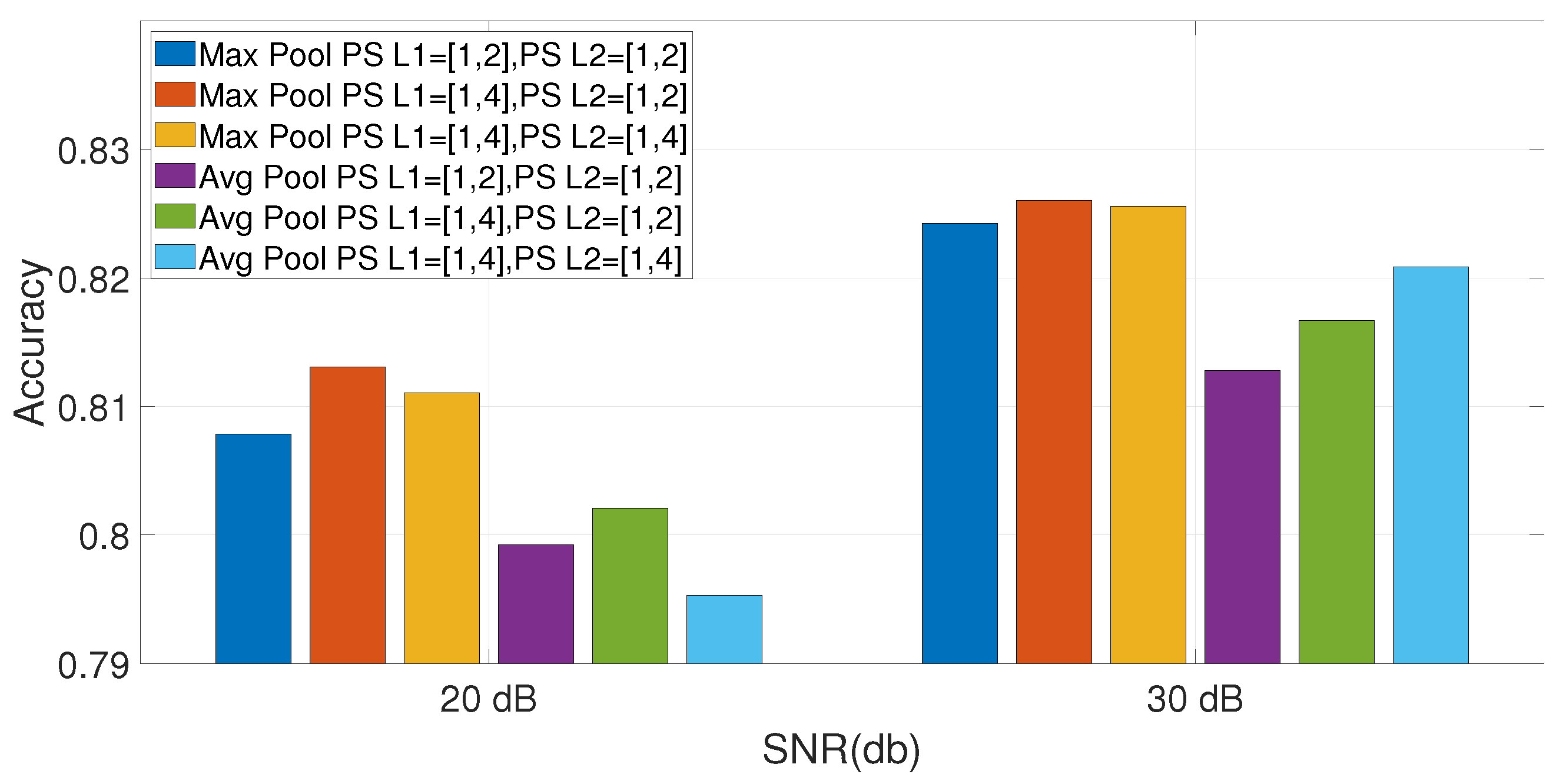
6.1. Parameters Optimization

This section provides some examples of the optimization of the hyperparameters of the approach and of the CNN. The most significant hyperparameter in the approach is the segment size $Op{t}_{seg}$ (the possible values are 32, 64, 128, 256, and 512, and all 2048 samples) of the WHT representation. The approach tries to exploit the WHT property of the compact representation of a signal to reduce the dimension of the input data provided to the CNN, while preserving the identification accuracy and robustness in the presence of noise. For this reason, the evaluation is performed for different values of SNR in dB. It is also evaluated as to whether it is better to use only one of the voltage signals (Voltage A or Voltage B, as was done in [5]) or both of them because they are theoretically symmetric, even if nonlinearities in the ECU transceivers circuits may create some differences.

Figure 4 shows the comparison of the accuracy trends for different values of segment size $Op{t}_{seg}$ (indicated as a multiple of 2 for the combination of Voltage A and Voltage B) for different values of SNR in dB. The first finding is that with decreasing SNR values in decibels, the identification accuracy decreases. This is not surprising because with an increasing presence of noise, the CNN is not able to distinguish the different ECUs properly. On the other side, it can be seen that the choice of a smaller value of $Op{t}_{seg}$ (e.g., $Op{t}_{seg}=32$) does not only decreases the computing effort by the CNN, but also increases the robustness of the approach against the presence of noise. In fact, the accuracy trends with $Op{t}_{seg}=32$ and $Op{t}_{seg}=64$ show a significantly higher robustness of the algorithm than with higher values of $Op{t}_{seg}$. On the other hand, in the absence of noise, the accuracy obtained with $Op{t}_{seg}=64$ is slightly higher than with $Op{t}_{seg}=32$ (the details of the obtained values of accuracy and F-score are shown in

Table 2. Detailed report on the comparison of the different approaches. Both voltage A and voltage B have been used.

Approach	Accuracy	F-Score
SNR = 30 dB
CNN WHT $Op{t}_{seg}=32\ast 2$	0.826	0.810
CNN WHT $Op{t}_{seg}=64\ast 2$	0.835	0.820
CNN WHT all	0.781	0.780
CNN FFT Seg = 250 * 2	0.783	0.781
CNN FFT all	0.768	0.764
CNN DHT Seg = 250 * 2	0.709	0.710
CNN DHT all	0.614	0.614
CNN Time domain all (A+B) [4]	0.771	0.765
LSTM WHT $Op{t}_{seg}=32\ast 2$ [14]	0.811	0.807
DT WHT $Op{t}_{seg}=32\ast 2$	0.803	0.800
KNN WHT $Op{t}_{seg}=32\ast 2$	0.770	0.760
DT Stat.Feat. (inspired by [5,13])	0.635	0.628
KNN Stat.Feat. (inspired by [5,13])	0.537	0.528
SNR = 10 dB
CNN WHT $Op{t}_{seg}=32\ast 2$	0.619	0.608
CNN WHT $Op{t}_{seg}=64\ast 2$	0.613	0.597
CNN WHT All	0.450	0.449
CNN FFT Seg = 250 * 2	0.205	0.203
CNN FFT All	0.146	0.146
CNN DHT Seg = 250 * 2	0.270	0.263
CNN DHT All	0.200	0.194
CNN Time domain all (A+B) [4]	0.292	0.286
LSTM WHT $Op{t}_{seg}=32\ast 2$ [14]	0.572	0.568
DT WHT $Op{t}_{seg}=32\ast 2$	0.500	0.498
KNN WHT $Op{t}_{seg}=32\ast 2$	0.346	0.344
DT Stat.Feat. (inspired by [5,13])	0.06	0.06
KNN Stat.Feat. (inspired by [5,13])	0.04	0.04
SNR = 0 dB
CNN WHT $Op{t}_{seg}=32\ast 2$	0.290	0.264
CNN WHT $Op{t}_{seg}=64\ast 2$	0.255	0.242
CNN WHT All	0.167	0.168
CNN FFT Seg = 250 * 2	0.047	0.045
CNN FFT All	0.034	0.034
CNN DHT Seg = 250 * 2	0.111	0.104
CNN DHT All	0.081	0.079
CNN Time domain all [4]	0.132	0.129
LSTM WHT $Op{t}_{seg}=32\ast 2$ [14]	0.270	0.262
DT WHT $Op{t}_{seg}=32\ast 2$	0.240	0.237
KNN WHT $Op{t}_{seg}=32\ast 2$	0.128	0.118
DT Stat.Feat. (inspired by [5,13])	0.02	0.02
KNN Stat.Feat. (inspired by [5,13])	0.02	0.02

). Figure 4 also shows that the accuracy trend obtained with only Voltage A or Voltage B is significantly worse than with the combination of Voltage A and Voltage B. Then, it is preferable to consider both voltage signals, even if this doubles the size of the input to the CNN. It is also noted that the accuracy trend obtained with Voltage A is slightly better than the accuracy trends obtained with Voltage B.

Regarding the optimization of the CNN, an overview of the tuning of all the hyperparameters identified in Section 5.1 would take too much space from this paper. As an example, we provide the optimization of two of the most significant parameters in the CNN architecture: the Initial Learning Rate IRL and the pooling size. The IRL hyper-parameter controls how much to change the model in response to the estimated error each time the model weights are updated. As in the previous case with the $Op{t}_{seg}$ optimization, the evaluation is performed for different values of SNR in dB. The bar graph in Figure 5 shows the accuracy obtained at different values of SNR in dB. A value of $Op{t}_{seg}=64\ast 2$ with both Voltage A and B was used to perform the analysis. The general trend observed is that a value of IRL = 0.0005 provides better accuracy results (even if training may take longer), especially in the presence of noise. At SNR = 25 dB, an IRL value of 0.001 is slightly better than IRL = 0.0005. At SNR = 20 dB, a value of IRL = 0.01 produces results that are similar to IRL = 0.0005, but for most of the SNR values, IRL = 0.0005 provides the highest or a competitive accuracy.

The second hyper-parameter is the pooling size, which involves selecting a pooling operation, much like a filter to be applied to feature maps. The size of the pooling operation or filter is smaller than the size of the feature map. The optimization analysis in this study has considered two kinds of pooling algorithms: the max pooling, which performs downsampling by dividing the input into 1D pooling regions, then computing the maximum of each region and the average pooling, which performs downsampling by dividing the input into 1D pooling regions, then computing the average of each region. Three set pooling sizes have been selected in both cases for the two layers: (1) Layer 1 [1,2] and Layer 2 [1,2]; (2) Layer 1 [1,4] and Layer 2 [1,2]; and (3) Layer 1 [1,4] and Layer 2 [1,4]. As mentioned before, the optimal performance is obtained with the second option and the max pooling, as shown in Figure 6 below. For clarity (because the accuracy differences are less relevant than in other figures), only the accuracy values at SNR = 20 dB and SNR = 30 dB are reported in this figure. It can be seen that accuracy obtained with the average pooling is substantially lower than the one obtained with the max pooling.

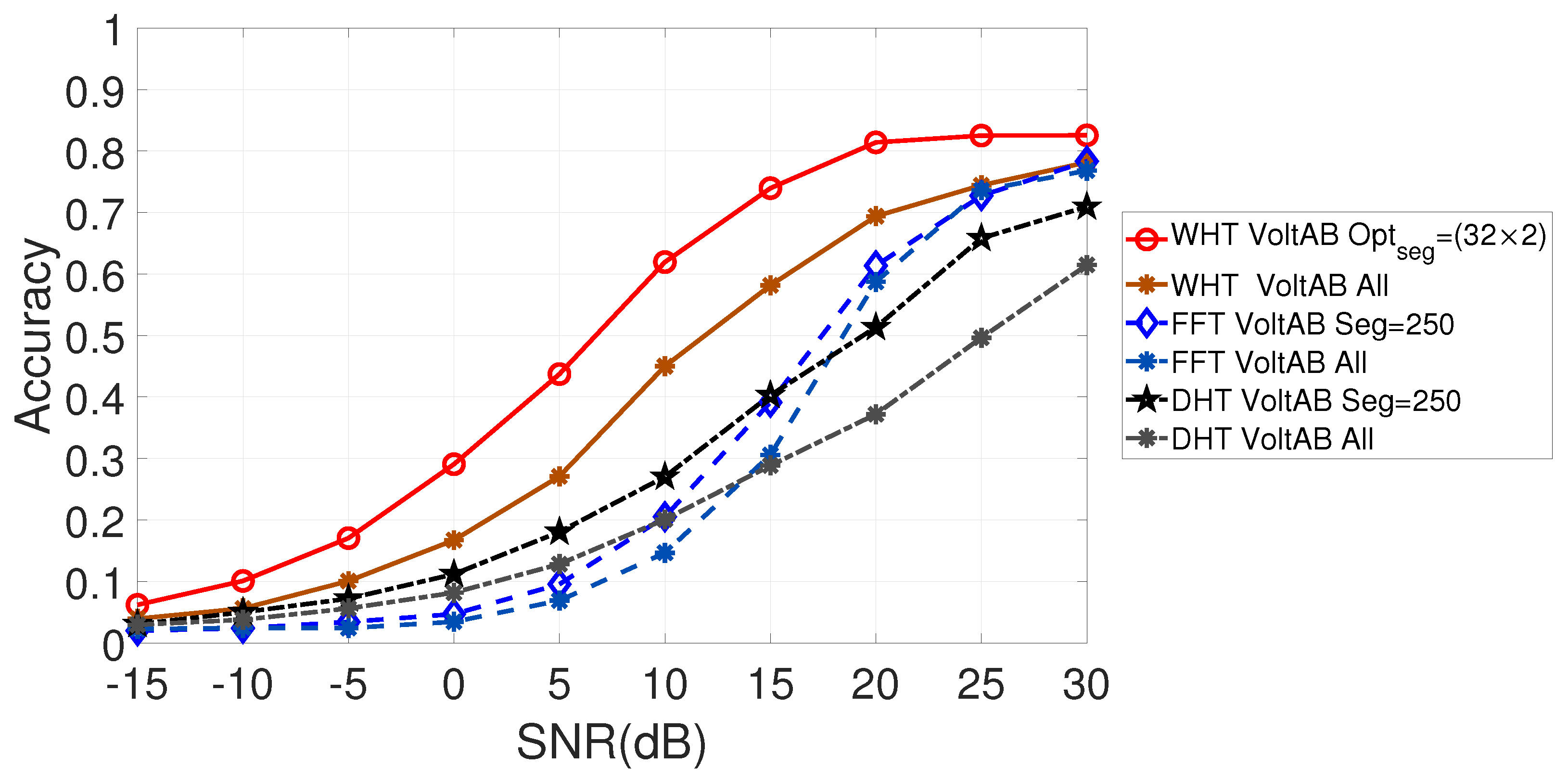
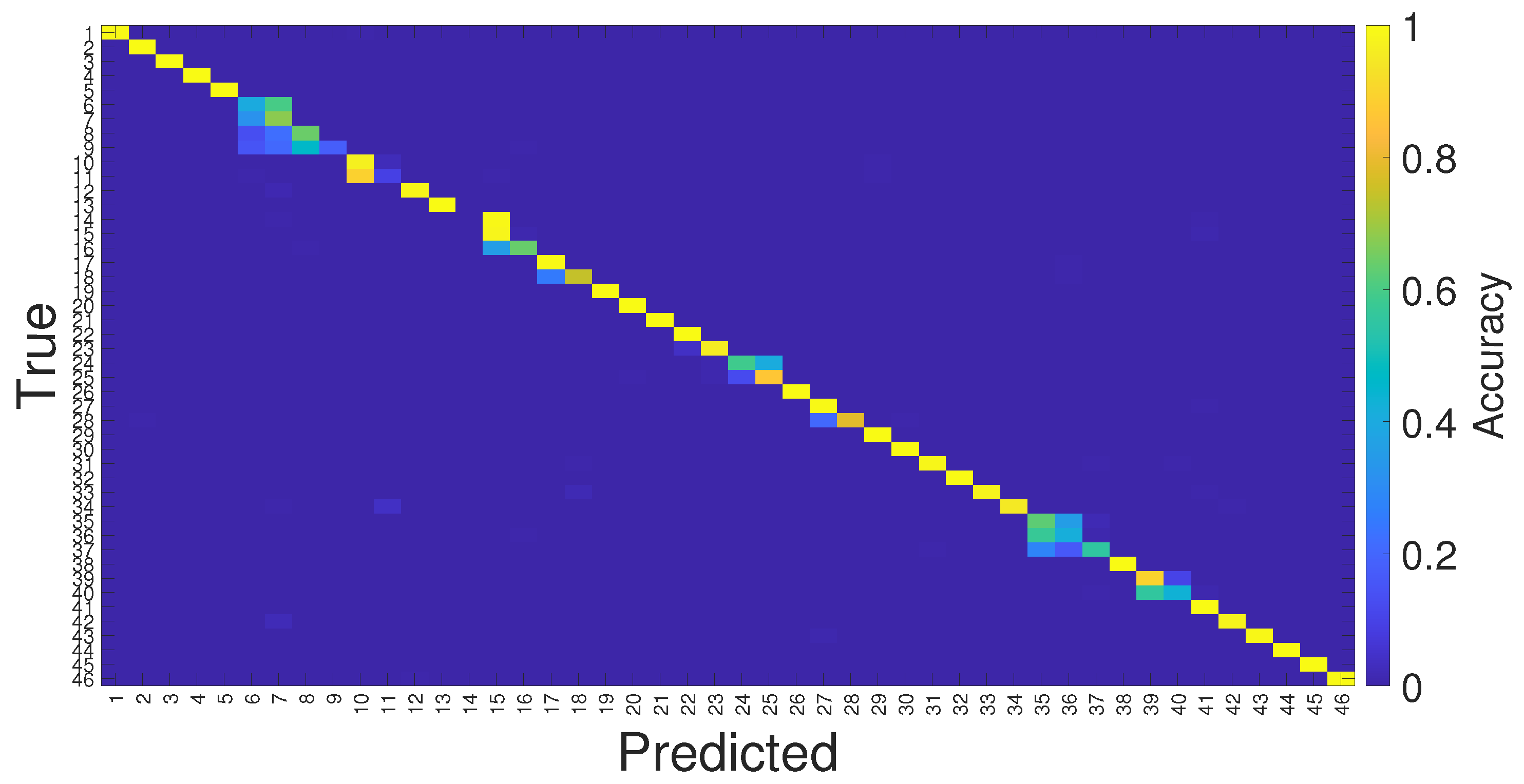
6.2. Comparison of the Approaches

This section presents a comparison of the proposed approach based on WHT with other approaches based on other transforms such as FFT or DHT. As in the previous cases, an evaluation is performed for different values of SNR in dB to analyze the impact of the presence of noise. The comparison of the approaches is shown in Figure 7. As can be seen from the picture, the approach based on WHT is significantly more robust than the other approaches, as the accuracy is much higher than that of FFT and DHT. Only for values of SNR = 30 dB is the accuracy of the approach based on the FFT (amplitude component only) similar to the approach proposed based on WHT. A similar analysis of limiting the input to the CNN to a segment of the spectral presentation was also performed for FFT and DHT, with similar results. In particular, a segment size of 250 was considered for both FFT and DHT. The results show that this approach (which is basically a filtering in frequency) is able to limit the impact of noise because the discriminating features for the physical layer authentication are more concentrated in the lower frequency range. This result is not surprising for the characteristics of the ECU transceivers operating in the in-vehicle network, which mostly operate in a relatively (e.g., in comparison to wireless communication systems) low frequency range, and this is where the nonlinearities (exploited by the physical layer authentication technique) of the transceivers are more evident.

The comparison between the CNN algorithm, the LSTM algorithm, DT, and the KNN algorithms is shown in Figure 8, both for the case of WHT with $Op{t}_{seg}=32\ast 2$ (both voltages A and B), and for the statistical features approach. We note that the data set is normalized and synchronized compared to the original data set used in [5]. Then, the results presented in this paper for the statistical features approach are not directly comparable, also because the statistical features used in this paper are different. This article has used the following statistical features: mean, variance, skewness, kurtosis, Shannon entropy, and maximum value, which are inspired by the features used in both [5,13]. Figure 8 shows that the performance of the ’shallow’ ML algorithms is worse than the CNN, especially in the presence of noise. The combination of the “shallow” ML algorithms with the statistical features is even worse than the one using WHT. On the other side, the application of the LSTM algorithm provides a classification accuracy that is slightly inferior to the CNN.

While Figure 7 shows the comparison of WHT with the other linear transforms, Figure 9 shows the comparison of the accuracy trend obtained with WHT $Op{t}_{seg}=32\ast 2$ with the application of the CNN directly to the base time domain representation of the signal (as in [4]) for voltage A (i.e., CANH), voltage B (i.e., CANL), and the combination of voltage A and voltage B. As can be seen in Figure 9, the combination of WHT with CNN significantly outperforms the use of CNN directly on the original time signal, even in the presence of noise.

To complete this analysis of accuracy trends, Figure 10 shows the box plot obtained considering all of the classification results instead of only the mean, as shown in the previous figures. It can be noted that the results do not show a large variance and are quite cohesive.

The accuracy metric does not provide a complete assessment of the classification results for the balance between FP and FN. Then, in the following paragraphs and figures, other evaluation metrics are used to address this aspect: the confusion matrices and the F-score.

Figure 11 shows the confusion matrix for all 46 ECUs considered in this study, with $Op{t}_{seg}=64$ at SNR = 30 dB. The y-axis represents the true values, while the x-axis represents the predicted values. It can be seen that most of the ECUs are correctly identified (with diagonal values almost reaching 100% accuracy) but some ECUs are more difficult to distinguish from others: ECU 6 against 7, or ECU 35 against ECU 36. This is because these pairs of ECUs are of the same model. The identification of electronic devices of the same model (the so-called intra-model classification) is in general more difficult than the identification of electronic devices of different models (the so-called inter-model classification) because the design differences of transceivers (between different models) are more significant than the manufacturing or material differences (between the different devices of the same model).

These differences become more significant with approaches, which are less well-performing than the WHT based approach. Figure 12 shows the confusion matrix obtained at SNR = 30 dB with the FFT (amplitude only) and SEG = 250. It can be seen that there are more errors (FP and FN) than in Figure 11, and sets of ECUs (rather than pairs) such as ECUs 6,7,8.9 are more difficult to distinguish.

The addition of noise decreases even more significantly the capability of the proposed approach to classify the different ECUs even when using the WHT based approach.

Figure 13 shows the confusion matrix obtained at SNR = 10 dB, with $OP{T}_{seg}=32\ast 2$, with both voltages A and B. This value of $OP{T}_{seg}$ is chosen for this figure because it has a higher accuracy than $OP{T}_{seg}=64\ast 2$, as shown in Figure 4). It can be seen that the sets of ECUs of the same model and belonging to the same vehicle appear as squared clusters, with similar colors representing a relatively low identification accuracy (e.g., the cluster of ECUs is 26 to 31). This trend is even more visible for lower values of SNR in dB, as shown in Figure 14 obtained at SNR = 0 dB with $OP{T}_{seg}=32\ast 2$, where a large number of FP and FN are present for most of the ECUs used in this study.

The following Table 2 shows the detailed numerical values of accuracy and F-score for all the different approaches, and for the specific SNR values in dB. As mentioned before, the WHT based approach has a significantly higher identification performance in comparison to the other approaches. As has already been mentioned, the maximum identification value (in terms of accuracy and F-score) is obtained with the WHT-based approach with a hyperparameter value $Op{t}_{seg}=64$ at SNR = 30 dB, while $Op{t}_{seg}=32$, and the highest values of accuracy and F-score are obtained at SNR = 10 dB and SNR = 0 dB.

Considering that one of the benefits of the application of WHT is related to the compactness of the representation of data input provided to the CNN, the computing time is calculated for each of the proposed approaches, and a comparison is shown in

Table 3. Comparison of the computing time among the different approaches.

Approach	Time
CNN WHT $Op{t}_{seg}=32\ast 2$	1
CNN WHT $Op{t}_{seg}=64\ast 2$	1.034
CNN Time Voltage A	1.332
CNN Time Voltage B	1.298
CNN Time Voltage A+B	1.971
DT WHT $Op{t}_{seg}=32\ast 2$	0.712
KNN WHT $Op{t}_{seg}=32\ast 2$	0.546
DT Feature Based	0.459
KNN Feature Based	0.32

. The computing time is presented as multiples of the time required to execute the CNN algorithm with the WHT $Op{t}_{seg}=32\ast 2$. The presented times in Table 3 include both the time to execute the DL/ML algorithm and the time needed to apply the transform (i.e., WHT) or the features, but it was found that the latter are negligible compared to the execution of DL/ML. In particular, the time to execute the WHT on all 46,000 samples of the data set is only 0.002 of the CNN WHT $Op{t}_{seg}=32\ast 2$ time (0.002 on the unitary time). Similarly, the time to execute the application of statistical features is 0.0037 in the ML feature based approach.

7. Conclusions and Future Developments

This paper has investigated the application of WHT in combination with CNN to the problem of the physical layer identification (also fingerprinting) of ECUs to counter cybersecurity threats. The WHT is known in the literature for image analysis, where its compactness of the image representation and its robustness in the presence of noise can benefit the image classification process. This study has applied WHT in one dimension only to the voltage output generated by the ECUs in the in-vehicle network. Because the detection of the physical layer fingerprints requires high sampling rates, the long (in terms of samples) one-dimensional voltage signal would generate a large data input for the CNN to process. The use of WHT allows for an efficient classification process because of the compactness property of WHT, where few sequence identifiers can be used. A comparison with transforms such as FFT and DHT shows that WHT is not only more efficient, but it achieves a higher identification accuracy even in the presence of noise.

Future developments of this study can investigate different research directions.

One direction would be to apply the combination of the Walsh–Hadamard Transform (WHT) with Convolutional Neural Networks (CNNs) to other electronic devices for physical layer authentication in the vehicle. For example, the combination of WHT and CNN can be used for the identification of the sensors used in the vehicle rather than the ECUs, as in this study.

Another direction is to enhance the WHT by dividing the ECU voltage time signal into shorter segments of equal length, and then to compute the WHT separately on each shorter segment. This is a similar concept to the definition of the Short-Time Fourier transform (STFT) in relation to the Fast Fourier Transform (FFT), which has demonstrated an enhanced physical layer authentication in the literature.

Finally, another research direction is to evaluate unsupervised learning approaches. Even if the public data set used in this paper is quite large in terms of the number of devices (i.e., 46), the application of unsupervised learning can be applied to evaluate the generalization capability of the proposed approach based on WHT and CNN or other Deep Learning algorithms such as the autoencoders.

References

1. Miller, C.; Valasek, C. Remote Exploitation of an Unaltered Passenger Vehicle; Black Hat: San Francisco, CA, USA, 2015. [Google Scholar]
2. Ebert, C.; Favaro, J. Automotive software. IEEE Softw. 2017, 34, 33–39. [Google Scholar] [CrossRef]
3. Petit, J.; Shladover, S.E. Potential cyberattacks on automated vehicles. IEEE Trans. Intell. Transp. Syst. 2014, 16, 546–556. [Google Scholar] [CrossRef]
4. Jeong, W.; Han, S.; Choi, E.; Lee, S.; Choi, J.W. CNN-based adaptive source node identifier for controller area network (CAN). IEEE Trans. Veh. Technol. 2020, 69, 13916–13920. [Google Scholar] [CrossRef]
5. Popa, L.; Groza, B.; Jichici, C.; Murvay, P.S. ECUPrint—Physical Fingerprinting Electronic Control Units on CAN Buses Inside Cars and SAE J1939 Compliant Vehicles. IEEE Trans. Inf. Forensics Secur. 2022, 17, 1185–1200. [Google Scholar] [CrossRef]
6. Soltanieh, N.; Norouzi, Y.; Yang, Y.; Karmakar, N.C. A review of radio frequency fingerprinting techniques. IEEE J. Radio Freq. Identif. 2020, 4, 222–233. [Google Scholar] [CrossRef]
7. Jian, T.; Rendon, B.C.; Ojuba, E.; Soltani, N.; Wang, Z.; Sankhe, K.; Gritsenko, A.; Dy, J.; Chowdhury, K.; Ioannidis, S. Deep learning for RF fingerprinting: A massive experimental study. IEEE Internet Things Mag. 2020, 3, 50–57. [Google Scholar] [CrossRef]
8. Zhao, Y.; Xun, Y.; Liu, J. ClockIDS: A Real-time Vehicle Intrusion Detection System Based on Clock Skew. IEEE Internet Things J. 2022, 9, 15593–15606. [Google Scholar] [CrossRef]
9. Cho, K.T.; Shin, K.G. Fingerprinting electronic control units for vehicle intrusion detection. In Proceedings of the 25th USENIX Security Symposium (USENIX Security 16), Austin, TX, USA, 10–12 August 2016; pp. 911–927. [Google Scholar]
10. Ying, X.; Sagong, S.U.; Clark, A.; Bushnell, L.; Poovendran, R. Shape of the cloak: Formal analysis of clock skew-based intrusion detection system in controller area networks. IEEE Trans. Inf. Forensics Secur. 2019, 14, 2300–2314. [Google Scholar] [CrossRef] [Green Version]
11. Choi, W.; Joo, K.; Jo, H.J.; Park, M.C.; Lee, D.H. Voltageids: Low-level communication characteristics for automotive intrusion detection system. IEEE Trans. Inf. Forensics Secur. 2018, 13, 2114–2129. [Google Scholar] [CrossRef]
12. Choi, W.; Jo, H.J.; Woo, S.; Chun, J.Y.; Park, J.; Lee, D.H. Identifying ecus using inimitable characteristics of signals in controller area networks. IEEE Trans. Veh. Technol. 2018, 67, 4757–4770. [Google Scholar] [CrossRef]
13. Kneib, M.; Huth, C. Scission: Signal characteristic-based sender identification and intrusion detection in automotive networks. In Proceedings of the 2018 ACM SIGSAC Conference on Computer and Communications Security, Toronto, ON, Canada, 15–19 October 2018; pp. 787–800. [Google Scholar]
14. Yang, Y.; Duan, Z.; Tehranipoor, M. Identify a spoofing attack on an in-vehicle CAN bus based on the deep features of an ECU fingerprint signal. Smart Cities 2020, 3, 17–30. [Google Scholar] [CrossRef] [Green Version]
15. Pan, H.; Badawi, D.; Chen, C.; Watts, A.; Koyuncu, E.; Cetin, A.E. Deep Neural Network With Walsh-Hadamard Transform Layer for Ember Detection During a Wildfire. In Proceedings of the IEEE/CVF Conference on Computer Vision and Pattern Recognition, Vancouver, BC, Canada, 18 June 2022; pp. 257–266. [Google Scholar]
16. Badawi, D.; Agambayev, A.; Ozev, S.; Cetin, A.E. Real-time low-cost drift compensation for chemical sensors using a deep neural network with hadamard transform and additive layers. IEEE Sensors J. 2021, 21, 17984–17994. [Google Scholar] [CrossRef]
17. SAE J1939-21; Data Link Layer. SAE International: Warrendale, PN, USA, 2001.
18. Hell, M.M. The physical layer in the CAN FD world-The update. In Proceedings of the Introduction to the Controller Area Network Conference, Washington, DC, USA, 23–25 January 2015; pp. 1–2. [Google Scholar]
19. Othman, H.; Aji, Y.; Fakhreddin, F.; Al-Ali, A. Controller area networks: Evolution and applications. In Proceedings of the 2006 2nd International Conference on Information & Communication Technologies, Damascus, Syria, 24–28 April 2006; IEEE: New York, NY, USA, 2006; Volume 2, pp. 3088–3093. [Google Scholar]
20. Reising, D.; Cancelleri, J.; Loveless, T.D.; Kandah, F.; Skjellum, A. Radio identity verification-based IoT security using RF-DNA fingerprints and SVM. IEEE Internet Things J. 2020, 8, 8356–8371. [Google Scholar] [CrossRef]
21. Baldini, G.; Giuliani, R.; Gemo, M. Mitigation of Odometer Fraud for In-Vehicle Security Using the Discrete Hartley Transform. In Proceedings of the 2020 11th IEEE Annual Ubiquitous Computing, Electronics & Mobile Communication Conference (UEMCON), New York, NY, USA, 28–31 October 2020; IEEE: New York, NY, USA, 2020; pp. 0479–0485. [Google Scholar]
22. Beauchamp, K.G. Applications of Walsh and Related Functions, with an Introduction to Sequency Theory; Academic Press: Cambridge, MA, USA, 1984; Volume 2. [Google Scholar]
23. Fino, B.J.; Algazi, V.R. Unified matrix treatment of the fast Walsh-Hadamard transform. IEEE Trans. Comput. 1976, 25, 1142–1146. [Google Scholar] [CrossRef]
24. Hosseini-Nejad, H.; Jannesari, A.; Sodagar, A.M. Data compression in brain-machine/computer interfaces based on the Walsh–Hadamard transform. IEEE Trans. Biomed. Circuits Syst. 2013, 8, 129–137. [Google Scholar] [CrossRef]
25. Sneha, P.; Sankar, S.; Kumar, A.S. A chaotic colour image encryption scheme combining Walsh–Hadamard transform and Arnold–Tent maps. J. Ambient Intell. Humaniz. Comput. 2020, 11, 1289–1308. [Google Scholar] [CrossRef]
26. Elliott, D.F.; Rao, K.R. Fast Transforms Algorithms, Analyses, Applications; Elsevier: Amsterdam, The Netherlands, 1983. [Google Scholar]
27. Bracewell, R.N. Discrete hartley transform. JOSA 1983, 73, 1832–1835. [Google Scholar] [CrossRef]
28. Waibel, A.; Hanazawa, T.; Hinton, G.; Shikano, K.; Lang, K.J. Phoneme recognition using time-delay neural networks. IEEE Trans. Acoust. Speech Signal Process. 1989, 37, 328–339. [Google Scholar] [CrossRef]
29. Zhang, W.; Tanida, J.; Itoh, K.; Ichioka, Y. Shift-invariant pattern recognition neural network and its optical architecture. In Proceedings of the Annual Conference of the Japan Society of Applied Physics, Tokyo, Japan, 24–26 August 1988; pp. 2147–2151. [Google Scholar]
30. Li, Z.; Liu, F.; Yang, W.; Peng, S.; Zhou, J. A survey of convolutional neural networks: Analysis, applications, and prospects. IEEE Trans. Neural Netw. Learn. Syst. 2021, 33, 6999–7019. [Google Scholar] [CrossRef]
31. Scherer, D.; Müller, A.; Behnke, S. Evaluation of pooling operations in convolutional architectures for object recognition. In Proceedings of the International Conference on Artificial Neural Networks, Thessaloniki, Greece, 15–18 September 2010; Springer: Berlin/Heidelberg, Germany, 2010; pp. 92–101. [Google Scholar]
32. Zafar, A.; Aamir, M.; Mohd Nawi, N.; Arshad, A.; Riaz, S.; Alruban, A.; Dutta, A.K.; Almotairi, S. A Comparison of Pooling Methods for Convolutional Neural Networks. Appl. Sci. 2022, 12, 8643. [Google Scholar] [CrossRef]
33. Hochreiter, S.; Schmidhuber, J. Long short-term memory. Neural Comput. 1997, 9, 1735–1780. [Google Scholar] [CrossRef] [PubMed]
34. Cover, T.; Hart, P. Nearest neighbor pattern classification. IEEE Trans. Inf. Theory 1967, 13, 21–27. [Google Scholar] [CrossRef] [Green Version]
35. Loh, W.Y. Classification and regression trees. Wiley Interdiscip. Rev. Data Min. Knowl. Discov. 2011, 1, 14–23. [Google Scholar] [CrossRef]
Figure 1. Overall workflow of the proposed approach.
Electronics 12 00199 g001
Figure 2. Examples of the Voltage A and Voltage B signals, and their WHT transforms. (a) Example of CANH-Voltage A. (b) WHT Voltage A. (c) Example of CANL-Voltage B. (d) WHT Voltage B.
Electronics 12 00199 g002
Figure 3. Architecture of the Convolutional Neural Network used in the study for the WHT, FFT, and DHT representations.
Electronics 12 00199 g003
Figure 4. Accuracy trends with CNN and WHT with different values of O p t s e g and for different values of SNR in dB. When both voltage signals are used, O p t s e g is indicated as multiplied by 2 in the figure.
Electronics 12 00199 g004
Figure 5. Accuracy trends with CNN for different values of the Initial Learning Rate (IRL) and different values of SNR in dB with O p t s e g = 64 .
Electronics 12 00199 g005
Figure 6. Impact of the pooling size and algorithms on the accuracy with CNN and WHT for SNR = 20 dB and SNR = 30 dB. PS means the Pooling Size, L1 indicates the first pooling layer, L2 indicates the second pooling layer.
Electronics 12 00199 g006
Figure 7. Accuracy trends with CNN for the different tranforms (WHT, FFT, and DHT) and different values of SNR in dB.
Electronics 12 00199 g007
Figure 8. Comparison of the accuracy trends of CNN WHT for O p t s e g = 32 2 for different values of SNR in dB with the LSTM algorithm, and the DT and KNN algorithms on WHT for O p t s e g = 32 2 , and with the DT and KNN algorithms with the feature based approach.
Electronics 12 00199 g008
Figure 9. Comparison of the approach based on CNN with WHT and O p t s e g = 32 2 (Voltage A and B), and CNN with the original time domain voltage signal for Voltage A, B, and the combination of Voltage A and B for different values of SNR in dB.
Electronics 12 00199 g009
Figure 10. Box Plot obtained with WHT and O p t s e g = 32 2 (Voltage A and B) for different values of SNR in dB.
Electronics 12 00199 g010
Figure 11. Confusion matrix with WHT and O p t s e g = 64 at SNR = 30 dB.
Electronics 12 00199 g011
Figure 12. Confusion matrix with FFT at SNR = 30 dB.
Electronics 12 00199 g012
Figure 13. Confusion matrix with WHT and O p t s e g = 32 at SNR = 10 dB.
Electronics 12 00199 g013
Figure 14. Confusion matrix with WHT and O p t s e g = 32 at SNR = 0 dB.
Electronics 12 00199 g014