Load Restoration Flexible Optimization in Wind Power Integrated System Based on Conditional Value at Risk

Abstract

In order to better accommodate the uncertainty induced from a high penetration of wind power during load recovery, a method of load restoration flexible optimization is developed in this paper. First, the idea of adopting flexible operational constraints when optimizing schemes is presented so as not to be too conservative in the application of wind power output during restoration. Further, conditional value at risk (CVaR) is employed to define an operational constraint slacking factor (OCSF) through analyzing the extent of constraint exceeding the prescribed limits when wind speed is taking the value outside its confidence interval. Adopting OCSF, a mixed integer linear programming (MILP) model of flexible load restoration, is constructed based on the primary model by substituting adjustable constraints for rigid constraints, which can be solved with CPLEX. Finally, the New England 10-unit 39-bus power system is used to demonstrate the proposed method, and the results explicitly indicate that the amount of load picked up can be effectively increased and an operational security can be guaranteed as well.

1. Introduction

The interconnection of regional power grids provides the platform for realizing the balance between the power supply and load in a wider range [1]. Under the background of green and low-carbon transformation of energy production and consumption, the amount of renewable energy, such as wind and solar, connecting with the power system is increasing sharply. Due to the inherent intermittency and volatility of renewable energy output, the regulation and operation safety of a power system is faced with huge potential risk. Particularly, the high-impact, low-probability extreme weather phenomenon remains a significant threat to power system reliability [2]. The experiences of unexpected disasters around the globe have warned us of the horrible economic loss and social impact caused by a system outage [3,4] so that the coping strategy to power a system blackout in case of catastrophes has become a demanding issue [5].

To address the above issues, the concept of “resilience” is introduced into electrical power territory. For the electrical power system with resilience, or a resilient system, it should be qualified with key features of resistance, redundancy, and recovery ahead, during, and after the event, respectively, which means the system is resistant to withstand initial shock, being capable of minimizing the damage for the duration and self-organized to a normal state as soon as possible post event [1]. As an important component of power system resilience, how to improve system restorability after large-scale power failure has drawn more attention. Besides infrastructure reinforcement, optimizing the strategies of dispatching and operation have been recognized as a preferred choice for improving the restorability of the existing grid [6,7].

Black start following the large-scale outage is critical to increase the restorability, which is an important part of the concept of a power system resilience [8]. With the help of cranking power provided by black start unit, the general black start operation usually is the first start to key generator sets carrying a basic load and energizing the skeleton network so as to pick up a load rapidly and comprehensively [9]. Lack of cranking power always remains a large obstacle to quick recovery following a massive outage. Wind power has the advantages of rapid startup, flexible adjustment, and less auxiliary power. In the context of large-scale wind power being connected with transmission network, wind power is expected to become a powerful supplement to cranking power. It is exciting that a more effective control of wind turbine (WT) has provided a broad prospect for the better employment of wind power in black start. The grid connected WTs’ low-voltage-ride-through capability is enhanced significantly during a network disturbance by means of the energy capacitor system [10]. Reference [11] reveals inherent deficiency of WT for system restoration and identifies the prerequisites for WT providing cranking power. Taking the advantage of WT’s quick start, the complete optimal restoration sequence, including units, transmission paths, and load pick-up, is obtained in [12] to minimize the restoration duration as well as improve the sustainability of the system. To improve reliability and availability of a restoration scheme in an extreme adverse scenario of wind power output, the information gap decision theory is adopted in [13] to construct a robust model for recovering the distribution system optimally. At the level of transmission network, the general requirements for the proportion of wind output in the recovery are given in the restoration plans of PJM and Ontario power systems [14,15]. In order to evaluate the limit of wind power connected with a system at a certain stage of the restoration, Ref. [16] defines the concept of dynamic wind power penetration limit (DWPPL), and a further solution based on chance constrained programming (CCP) is provided to making black start scheme, taking wind power into consideration. Stochastic programming based on scenarios is introduced in [17] in order to deal with the uncertainty of wind output, where scenarios are filtered and clustered so as to obtain a reduced computational load and an offline recovery scheme considering the wind power is achieved. Furthermore, the online restoration process considering wind power participation is investigated using the two-stage robust method in [18], and the coordination between wind farm and pumped storage to support recovery is studied in [19]. In the case of known confidence of wind speed prediction, Ref. [20] adopts the method of conditional value at risk (CVaR) to investigate the potential risk of wind fluctuation beyond confidence interval to performance of restoration scheme. Further, the bi-level load restoration optimization model is constructed to manage restoration risk according to the dispatching reference.

On the whole, existing research work related to load restoration focuses mainly on the innovation of load restoration modeling to accommodate as much uncertainty induced from wind power as possible. Nevertheless, it is common for existing methods to adopt rigid operational constraints in modeling. By contrast, this paper proposed a method of load restoration flexible optimization, where operational constraints can be slacked within the allowable security range when wind output disturbances beyond the confidence level occur in a short time so that the wind power can be employed fully to maximize the amount of load unserved.

The contents of this paper are arranged as follows: The framework of load restoration flexible optimization is given in Section 2. The core of load restoration flexible optimization, namely the concept of operational constraint slacking factor (OCSF), is given in Section 3. Based on the definition of CVaR, the OCSF is further derived from analysis of constraints exceeding the prescribed constraint limits when wind speed is outside its confidence interval. Taking the advantage of fast decoupled power flow and sensitivity analysis, flexible optimization of load restoration is modeled as a MILP problem with OCSF in Section 4, and a corresponding algorithm flow is given as well. New England 10-unit 39-bus power system is used to simulate in Section 5, and detailed results reveal the effectiveness of proposed method. Finally, the conclusion is given in Section 6.

2. Framework of Load Restoration Flexible Optimization

Under the circumstance of high renewable energy penetration, the concept of flexibility has been commonly recognized in the planning and operation of a power system [21]. Flexible optimization seeks for the comprehensive optimal solution to improve the adaptability of schemes to various uncertain parameters, which meets the power system resilient request perfectly [22]. The flexibility theory was applied in a flexible AC transmission system (FACTS) and power grid planning when initially introduced into electric power field [23,24]. Flexible network planning takes the uncertain factors into consideration to formulate the synthetically optimal scheme to minimize the general economic investment [25], which means the scheme formulated may sacrifice some less-probable scenes or even break the operation constraints under some extreme circumstances. The similar opinion could be grafted into wind-power-integrated load restoration. According to spot experiment results, network infrastructures, such as transmissions and transformers are capable of working in an overloaded state [26]. System indices, such as bus voltage and system frequency, could breakthrough security constraints under some circumstances as well [27]. Based on this, since load restoration speed is the primary concern, it is promising to loosen the operation constraints scientifically and reasonably according to wind speed and network situation, to further enhance the load restoration ability with the adaption of wind power. The framework of load restoration flexible optimization is demonstrated as Figure 1.

As shown in Figure 1, load restoration flexible optimization mainly consists of three key steps, namely the formation of initial load restoration scheme (LRS), solution of flexible constraints and determination of final flexible LRS. Improvement of the resilience of LRS means that LRS made should be able to accommodate the disturbance of wind output within and beyond the confidence. Therefore, initial schemes are optimized based on the forecasting wind speed within confidence, which is realized through the primary model adopting the regular rigid constraints. The availability of the initial LRS must be validated under the scenario of wind power output fluctuation beyond the confidence. The common practice is to abandon the original LRS or reduce the load recovery amount once the rigid constraint is broken, which may lead to a conservative scheme and restrict the speed of load recovery. To cope with this deficiency, this paper employs flexible constraints which are regulated by operational constraint slacking factor (OCSF) to accommodate the severe fluctuation of wind output with the small probability, which constitutes a flexible optimization model for load restoration. Among key steps, the core is definition of OCSF and its iterative solution based on wind speed beyond confidence, which will be explained in detail in Section 3.

3. Definition of OCSF Based on CVaR

3.1. Introduction of OCSF for Load Restoration

After massive outage, the complete load recovery is closely following generating capability restoration and network reconstruction. Generally, the load is picked up in several steps, and maximizing the amount of load picked up in each step is the primary objective so that the duration of restoration can be reduced. Meanwhile, operation constraints, such as transient frequency drop, bus voltage, transmission capacity, and generator output, should be satisfied as well as power flow balance. As a high penetration of wind power in system occurs, the possibility of constraints exceeding limits is increasing when making a restoration decision because of output fluctuation of wind power. In order to improve the resilience of restoration control, OCSF is introduced in making LRS.

It is assumed that prediction confidence of wind speed u is $\beta$, and its probability density distribution is $\rho (u)$. Accordingly, wind speed within and beyond confidence level $\beta$ are denoted with $[u_{\beta }]$ and ${[u_{\beta }]}^{+}$, as shown in Equation (1).

$$\left\{\begin{array}{l}[u_{\beta }]=\{u\in [u_{\min }^{\beta },u_{\max }^{\beta }]|{\displaystyle {\int }_{u_{\min }^{\beta }}^{u_{\max }^{\beta }}\rho (u)du=\beta }\}\\ [u_{\beta }{]}^{+}=\{u|u\le u_{\min }^{\beta }\}\cup \{u|u\ge u_{\max }^{\beta }\}\end{array}\right.$$

(1)

It is supposed that $f$ represents the optimization goal in making LRS. The rigid constraint, such as Equation (2) is effective when initial LRS is formulated with the participation of wind corresponding to $[u_{\beta }]$.

$$[{\delta }_{\beta }]=[{\delta }_b^{\beta },{\delta }_t^{\beta }]={\displaystyle \sum _{[u_{\beta }]}\cup [{\delta }_b(f_{\beta }),{\delta }_t(f_{\beta })]}$$

(2)

where $\delta$ is a unified representative of security indices, such as frequency, voltage, transmission capacity, and generation rated power. Subscript b and t are used to classify the lower and the upper limit of the rigid constraint. Taking the fluctuation of wind power corresponding to ${[u_{\beta }]}^{+}$ into consideration, the rigid constraint may be relaxed reasonably within the limit of extreme constraint to facilitate the adaptability of LRS. Accordingly, the slack constraint is completely expressed as Equation (3)

$$\left\{\begin{array}{l}[{\delta }_{\beta }{]}^{+}=[{\delta }_b^{\beta +},{\delta }_b^{\beta }]\cup [{\delta }_b^{\beta },{\delta }_t^{\beta }]\cup [{\delta }_t^{\beta },{\delta }_t^{\beta +}]\\ {\delta }_t^{\beta +}=(1+{\xi }_t){\delta }_t^{\beta }\\ {\delta }_b^{\beta +}=(1-{\xi }_b){\delta }_b^{\beta }\\ [{\delta }_{\beta }{]}^{+}\subseteq [{\delta }_{ex}]\end{array}\right.$$

(3)

where ${\xi }_t$ and ${\xi }_b$ are OCSFs corresponding to upper and lower constraints and $[{\delta }_{ex}]$ is the extreme constraint limit.

3.2. Derivation of OCSF Based on CVaR

As a tool for risk management in the field of financial economics, value at risk (VaR) can measure the maximal loss of portfolio under a certain confidence level. Accordingly, conditional value at risk (CVaR) is employed to estimate the loss expectation when the loss is exceeding VaR. In terms of load recovery, the risk can be understood as the extent to which operational constraint is broken when initial LRS is disturbed at the wind speed corresponding to ${[u_{\beta }]}^{+}$, which can be represented with Equation (4).

$$\left\{\begin{array}{l}{\xi }_t^{\beta +}=\frac{{\delta }_t^{\beta +}(f_{\beta },{[u_t^{\beta }]}^{+})-{\delta }_t^{\beta }}{{\delta }_t^{\beta }}\\ {\xi }_b^{\beta +}=\frac{{\delta }_b^{\beta }-{\delta }_b^{\beta +}(f_{\beta },{[u_b^{\beta }]}^{+})}{{\delta }_b^{\beta }}\end{array}\right.$$

(4)

Taking into account the randomness of wind conditions, the risk expectation can be expressed as Equation (5) by means of CVaR [28]. If taking the value within the maximum value permitted by extreme constraint limit $[{\delta }_{ex}]$, the risk expectation is namely OCSF.

$$\left\{\begin{array}{l}{\xi }_{CVaR}^{\beta ,t}=\frac{1}{1-\beta }{\displaystyle {\int }_{{\xi }_t^{\beta +}\ge 0}{\xi }_t^{\beta +}\rho (u_{\beta }^{t+})du},u_{\beta }^{t+}\in [u_{\beta }^t{]}^{+}\\ {\xi }_{CVaR}^{\beta ,b}=\frac{1}{1-\beta }{\displaystyle {\int }_{{\xi }_b^{\beta +}\ge 0}{\xi }_b^{\beta +}\rho (u_{\beta }^{b+})du},u_{\beta }^{b+}\in [u_{\beta }^b{]}^{+}\end{array}\right.$$

(5)

where ${[u_{\beta }^t]}^{+}$ and ${[u_{\beta }^b]}^{+}$ are used to distinguish wind speed, which may contribute to exceeding the upper limit and lower limit of the rigid constraint. Accordingly, $\rho ({[u_{\beta }^t]}^{+})$ and $\rho ({[u_{\beta }^b]}^{+})$ are their probability density.

4. Load Restoration Flexible Optimization

From the load restoration flexible optimization framework illustrated in Figure 1, it can be seen that load restoration flexible optimization is carried out on the base of initial LRS obtained previously. Therefore, the primary model of load restoration optimization for making initial LRS is constructed at first in this part and then the form of flexible optimization is proposed through employing OCSF. Finally, the flow of load restoration flexible optimization is provided to explain how the method is implemented.

4.1. Primary Model of Load Restoration Optimization

4.1.1. Objective Function

As previously mentioned, the complete load recovery phase following the blackout starts after the formation of the backbone grid. At this time, the synchronous generator sets can flexibly ramp up or down in terms of dispatching requirements. In other words, the topology of the grid remains unchanged during the process of load recovery and the main task is to optimize the sequence of picking up loads according to their priorities so that the loss of the power interruption can be reduced as much as possible. Generally, the objective of load restoration optimization is to maximize the value of load recovered, which is expressed by Equation (6).

$$\max f=CW\Delta {\mathit{P}}^D$$

(6)

where $\mathit{C}$ is 0–1 decision vector, in which an element takes the value 1, means that the corresponding load is picked up, otherwise it will not be recovered. $\Delta {\mathit{P}}^D$ is a vector denoting the load amount recovered in each time-step. $\mathit{W}$ is a diagonal matrix and the diagonal elements represent the comprehensive weight of corresponding load nodes. Generally, a load node is connected with loads of different importance levels and thus the comprehensive weight being denoted by Equation (7). ${\Omega }_D$ is the set of load nodes. $S_{i,\ast }$ is the proportion of the load with a different priority at node i, and $w_{\ast }$ is the corresponding weight.

$$W_i=S_{i, I}{w}_I+S_{i, II}{w}_{II}+S_{i, III}{w}_{III}, i\in {\Omega }_D$$

(7)

On the whole, the higher the comprehensive importance of nodes, the more likely they are to be recovered first. As for a specific node, the higher priority part of the load will be recovered first.

4.1.2. Operation Constraints

During load recovery, operation constraints must be met. Specifically, those constraints are transient frequency drop, bus voltage, transmission capacity, and generator output and power flow balance. Of all constraints, except for the transient frequency constraint, the satisfaction of other constraints shall be checked by power flow calculation. To simplify the solution, a power flow linearization method taking the leverage of fast decoupled power flow and sensitivity analysis is introduced in detail following the explanation of the transient frequency constraint.

Transient Frequency Constraint

In the process of load restoration, the load is picked up in batches step by step. The amount of load recovered in one step is up to the compromise between the restoration efficiency and the operation security. It is a common practice that the limit of transient frequency drop, namely $\Delta f_{\max }$, is used to determine the maximum amount of load picked up in one step, which is shown in Equation (8), where $\Delta P_i^D$ is the load amount recovered in load node i, $\Delta P_j^W$ is the power increment of wind farm j at the expected wind speed, and $P_{kN}^G$ and $d{f}_k$ are rated power and frequency response rate of synchronous generator k.

$${\displaystyle \sum _{i=1}^{N_D}\Delta P_i^D-{\displaystyle \sum _{j=1}^{N_W}\Delta P_j^W}\le \Delta f_{\max }{\displaystyle \sum _{k=1}^{N_G}\frac{P_{kN}^G}{d{f}_k}}}$$

(8)

Power Flow Linearization

Load restoration is composed of a series of sequential operations. In each step, picking up load and unit output regulation will cause changes in power flow, which should not exceed the prescribed limits of transmission capacity and bus voltage. It will facilitate the solution of load restoration that the constraints of transmission capacity and bus voltage are transformed into the constraints of active and reactive power output at buses.

The active power flow of a transmission line is affected by the active power injection at bus, as shown in Equation (9). $\Delta P_m^L$ is the active power increment of branch m. $\Delta P$ is the vector of bus active power increment being composed of wind power increment vector $\Delta {\mathit{P}}^W$, synchronous generator output increment vector $\Delta {\mathit{P}}^G$, and load recovery amount vector $\Delta {\mathit{P}}^D$. $x_m$ is the reactance of branch m, ${\mathit{M}}_m$ is the branch incidence vector, and ${\mathit{B}}_0$ is DC power flow calculation matrix.

$$\Delta P_m^L=\frac{1}{x_m}{M}_m{B}_0^{-1}\Delta P$$

(9)

The relationship of Equation (9) can be applied to the whole network and expressed as Equation (10) together with branch capacity constraint. $B^L$ is a diagonal matrix whose diagonal elements are reciprocal of branch reactance. ${\mathit{M}}^L$ is a network incidence matrix. $P_{\max }^L$ is the limit of transmission capacity.

$$-P_{\max }^L\le P^L+(B^L{M}^L{B}_0^{-1})\Delta P\le P_{\max }^L$$

(10)

During the load restoration, ramping of synchronous generator in each step needs to satisfy the constraint (11). $D_k$ and $r_k$ are the minimum output and ramping rate of synchronous generator, $\Delta t$ is the time-step duration. $P_{k, t-1}^G$ is the output of synchronous generator k at the initial time of the current time-step.

$$P_k^{G,up}=\left\{\begin{array}{cc}{P}_{k, t-1}^G+r_k\Delta t,& P_{k, t-1}^G<D_k\\ \min \{P_{kN}^G, P_{k, t-1}^G+r_k\Delta t\},& P_{k, t-1}^G\ge D_k\end{array}\right.$$

(11)

If the constraints of reserve capacity are further considered to deal with the fluctuation of wind power, the output of synchronous generator should meet Equations (12) and (13) where ${\Omega }_{Gup}$ denotes the set of synchronous generators reserved for upper adjustment, and $P_{r, up}^G$ is the reserved upward reserve capacity based on forecasting wind speed within the confidence level. Note that only upward reserve capacity of synchronous units is considered here in order to simplify restoration operation.

$$0\le \Delta P^G\le P_k^{G,\max }$$

(12)

$$P_k^{G,\max }=P_k^{G,up}-P_{r, up}^G\frac{r_k}{{\displaystyle \sum _{k\in {\mathsf{\Omega }}_{Gup}}{r}_k}}$$

(13)

Additionally, the active power balance constraint of the whole system must remain as Equation (14) where $E$ is a vector whose elements are all 1.

$$E\Delta P=0$$

(14)

During the load restoration, the reactive power injection of bus changes along with the active power injection of bus, which will cause a bus voltage fluctuation, so the voltage constraint as Equation (15) needs to be checked where $V$ and $\Delta V$ are, respectively, voltage vector and voltage increment vector of bus. $V_{\min }$ and $V_{\max }$ are the lower and upper limit of bus voltage.

$$V_{\min }\le V+\Delta V\le V_{\max }$$

(15)

According to fast decoupled power flow, $\Delta V$ and the reactive power injection increment of bus keep the relation as Equation (16). ${\mathit{B}}^{″}$ is an imaginary part of the admittance matrix except PV buses. Further, power factor constraint as Equation (17) in introduced to correlate reactive power injection of bus with active power injection of bus.

$$\Delta V=-{({\mathit{B}}^{″})}^{-1}\Delta Q$$

(16)

$$\Delta Q\le \Delta P\times \tan \alpha$$

(17)

Additionally, the reactive power balance constraint of the whole system must remain as Equation (18).

$$E\Delta Q=0$$

(18)

In summary, the primary model of load restoration optimization is organized as Equation (19).

$$\left\{\begin{array}{l}\max f=CW\Delta P^D\hfill \\ s.t. transient frequency constraint\hfill \\ \hspace{1em}\hspace{1em}active power constraints\hfill \\ \hspace{1em}\hspace{1em}voltage and reactive power constraints\hfill \end{array}\right.$$

(19)

where, transient frequency constraint refers to Equation (8), active power constraints include Equations (10)–(14), voltage and reactive power constraints include Equations (15)–(18).

4.2. Modeling of Load Restoration Flexible Optimization

Based on the primary model of load restoration optimization, initial LRS can be made. Initial LRS indicates load nodes to be recovered in a specific time-step and corresponding load amount picked up. Note that initial LRS is solved based on forecasting wind speed within the confidence level. When the scheme is put into operation, extreme wind conditions beyond the confidence level will bring about a corresponding adjustment of synchronous unit injection, which may further break relevant operation constraints, such as transmission capacity and bus voltage. On the condition the comprehensive risk caused by wind conditions beyond the confidence is controlled at a reasonable level, relaxation of operation constraints is beneficial to making full use of the load capacity of equipment and resilience improvement of initial LRS. Therefore, load restoration flexible optimization is modeled by introducing OCSF defined before.

The general expression of OCSF is given by Equation (5). Next, ${\xi }_f$, ${\xi }_P$, ${\xi }_G$, and ${\xi }_V$ are introduced successively in Equations (20)–(23), namely constraints of transient frequency drop, active power flow of transmission line, generator active power output, and bus voltage, where $E_P$ and $E_V$ are vectors whose elements take the value of 1, and the number of elements is equal to the branch number and bus number, respectively.

$${\displaystyle \sum _{i=1}^{N_D}\Delta P_i^D-{\displaystyle \sum _{j=1}^{N_W}\Delta P_j^W}\le (1+{\xi }_f)\Delta f_{\max }{\displaystyle \sum _{k=1}^{N_G}\frac{P_{kN}^G}{d{f}_k}}}$$

(20)

$$-(E_P+{\xi }_P^{\max })P_{\max }^L\le P^L+(B^L{M}^L{B}_0^{-1})\Delta P\le (E_P+{\xi }_P^{\max })P_{\max }^L$$

(21)

$$P_k^{G,up}=\left\{\begin{array}{cc}{P}_{k, t-1}^G+r_k\Delta t,& P_{k, t-1}^G<D_k\\ \min \left\{\right(1+{\xi }_G^{\max })P_{kN}^G, P_{k, t-1}^G+r_k\Delta t\},& P_{k, t-1}^G\ge D_k\end{array}\right.$$

(22)

$$(E_V-{\xi }_V^{\min })V_{\min }\le V+\Delta V\le (E_V+{\xi }_V^{\max })V_{\max }$$

(23)

In summary, the model of load restoration flexible optimization is organized as Equation (24).

$$\left\{\begin{array}{l}\max f=CW\Delta P^D\hfill \\ s.t. transient frequency constraint\hfill \\ \hspace{1em}\hspace{1em}active power constraints\hfill \\ \hspace{1em}\hspace{1em}voltage and reactive power constraints\hfill \end{array}\right.$$

(24)

where, transient frequency constraint refers to Equation (20), active power constraints include Equations (21), (22) and (12)–(14), voltage and reactive power constraints include Equations (23) and (16)–(18).

4.3. Flow of Load Restoration Flexible Optimization

Before making LRS with the proposed method in this paper, the requirement of wind power output being qualified for participating in load recovery must be confirmed first. In the load recovery phase following the blackout, if the fault occurs again due to improper operation or random disturbance, the load recovery process will be further delayed. Therefore, the scenario of excessive wind speed that may trigger the shutdown of wind power should be avoided in load recovery. Meanwhile, the wind power output less than 10 percent of rated power is suggested not to integrate with the system because it has a limited benefit for recovery. Moreover, the wind power output meeting the above output range should be able to last for a period of time, which is the minimum time guarantee for load recovery, such as 2 h. After that, the predicted wind conditions in the next 2–3 h are confirmed in terms of above requirements, and the LRS can be formulated according to the following flow.

Suppose that the probability distribution of wind speed prediction error is known, the Monte Carlo method is employed to obtain N numbers wind speed prediction error sequence (N is a large enough integer). Then, N numbers of wind conditions are obtained by superposing these sequences with the predicted wind speed sequence. When the range value of wind conditions is used to characterize the abominable degree of wind condition, the worst wind condition W_worst under a certain confidence level can be obtained. Thus, the better wind conditions than W_worst constitute the set within confidence (SWC), and the worst wind conditions than W_worst constitute the set beyond confidence (SBC).

On the whole, the flow of making LRS with OCSF is composed of three stages, namely, formation of initial LRS (ILRS), solution of OCSF, and generation of flexible LRS (FLRS) with OCSF. The detail of the flow is described as follows.

• At the given N, SWC and SBC are prepared according to the above method. Accordingly, wind power output corresponding to speed samples are obtained.
• Employing the primary model of load restoration optimization, namely Equation (19), initial LRS (ILRS) is optimized by adopting the wind power output corresponding to SWC.
• In order to observe the adaptability of ILRS to the adverse scenario of wind power, the disturbance corresponding to the wind power output from SBC is applied to ILRS, and the extent to which the constraints are broken is calculated. If the extent does not exceed the value prescribed by extreme constraint limit, the effective OCSF can be obtained with Equation (5).
• Using the model of load restoration flexible optimization, namely Equation (24), the FLRS is optimized by adopting all wind power output corresponding to SWC and SBC.

It should be noted that the above procedures are applicable to each step of load recovery and need to repeatedly be executed till complete load recovery.

5. Case Study

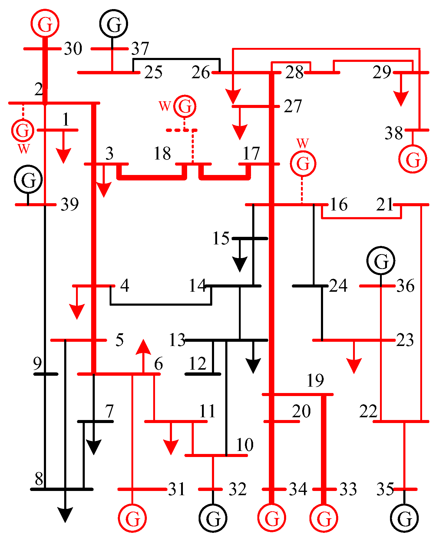
The proposed method is programmed in MATLAB and solved with CPLEX. Meanwhile, New England 10-unit 39-bus power system, as shown in Figure 2, is utilized to illustrate the performance of the proposed method.

Based on system configuration in [29], three wind farms are located at bus2, bus16, and bus18 where 200 double-fed induction generators with rated capacity of 1.5 MW are installed, respectively. For the sequence of picking a load for generators and classification of restoration steps, refer to [29]. Corresponding to Equation (7), $w_I$, $w_{II}$, and $w_{III}$ take the value of 1, 0.6, and 0.2, respectively. The amount and comprehensive weight of loads that need to be restored are listed in

Table 1. Amount and comprehensive weight of loads need to be restored.

Bus	Load Amount (MW)	Comprehensive Weight	Bus	Load Amount (MW)	Comprehensive Weight
1	220	0.526	13	160	0.548
3	320	0.540	15	320	0.591
4	500	0.557	23	250	0.570
6	120	0.520	26	370	0.536
7	240	0.482	27	280	0.588
8	520	0.584	29	340	0.522
11	230	0.573

. The marked red part in Figure 2 represents the energized network, and the bold branches can be overloaded.

5.1. Details Demonstration of Load Restoration Flexible Optimization

Take step 4 of load restoration as an example to demonstrate the performance of load restoration flexible optimization. The detailed information about making LRS without and with OCSF are given below. Firstly, the set of wind power, including 1000 samples, is acquired with the method described previously, in which the wind power prediction confidence degree is 70%. The amounts of load picked up corresponding to ILRS and FLRS are compared in

Table 2. Comparison of load amount recovered in step 4 between ILRS and FLRS (MW).

Bus	1	11	23	26	29	Total
ILRS	210.45	208.21	215.26	323.08	267.39	1224.39
FLRS	210.45	208.21	215.26	336.86	293.72	1264.5

. Accordingly, rigid and extreme constraints are checked, and results are list in

Table 3. Extent of rigid constraint satisfaction in step 4 corresponding to ILRS.

Security Index	Index Limit of Rigid Constraints	Index Extreme Value	Location of Extreme Value
transient frequency (Hz)	Upper: 50.5	50	-
	Lower: 49.5	49.57
bus voltage (p.u.)	Upper: 1.1	1.072	Bus-31
	Lower: 0.9	0.95	Bus-33
transmission capacity (MW)	Upper: PLN	PL17–18	L17–18
	Lower: 0	-	-
generator output (MW)	Upper: PGN	0.8932 PG-30	Gen-30
	Lower: 0	-	-

Note: The only restoration bottleneck of step 4 is the limit of transmission capacity of $L_{17-18}$.

and

Table 4. Extent of extreme constraint satisfaction in step 4 corresponding to FLRS.

Security Index	Index Limit of Extreme Constraints	Index Extreme Value with OCSF	Location of Extreme Value
transient frequency (Hz)	Upper: 50.5	50.5	-
	Lower: 48.5	49.5
bus voltage (p.u.)	Upper: 1.15	1.1	-
	Lower: 0.85	0.9	-
transmission capacity (MW)	Upper: 1.1 PLN	1.0683	L17–18
	Lower: 0	-
generator output (MW)	Upper: 1.05 PGN	1.0343 PG-34 1.0192 PG-38	Gen-34 Gen-38
	Lower: 0	-	-

, respectively.

From Table 2, it is obvious that the amount of load recovered with FLRS is improved a lot. The detailed reasons are explained as follows. Due to the difference of units’ ramping rate and uneven load distribution in whole system, it is necessary to pick up load located in the east of the system through increasing output of units in the west of the system according to ILRS of step 4. Associating the results of Table 3, the security index, such as transient frequency, bus voltage, and generator output, are within prescribed rigid constraints; the only bottleneck of step 4 is that the power transmission amount of $L_{17-18}$, reaching its upper limit, namely 900 MW.

On the basis of ILRS, load restoration flexible optimization proposed in this paper takes wind power output respecting the set beyond confidence into consideration and improves the resilience of load restoration through calculating OCSFs and slacking rigid constraint within permitted extreme constraints. Accordingly, the extreme value of the index after OCSF treatment is shown in Table 4. The security index, such as transient frequency and bus voltage, remain the same as the rigid constraints because the frequency drop and voltage variation are less than the prescribed deviation when a wind power output disturbance beyond confidence is imposed during picking up loads. However, the transmission capability of $L_{17-18}$ has been enlarged to 106.83%, and the output of Gen-34 and Gen-38 are adjusted to 103.43% and 101.92% of their rated output so that load recovery of Bus-26 and Bus-29 is increased by 40.11 WM in total as shown in Table 2. It is obvious that the performance of FLRS is improved a lot because the potential of generation and transmission capacity has been employed deeply. Note that operational security of FLRS still can be guaranteed due to the boundary of constraints regulated with OCSF not exceeding the extreme constraints.

5.2. Comparison of FLRS Corresponding to Different Confidence Degree of Wind Speed Prediction

Increasing the confidence degree of wind speed prediction to 90% to regenerate the relaxed constraints, the comparison of the constraints boundary is shown in Figure 3. Note fre, P_L, and P_G represent transient frequency, transmission capacity of line, and generator output. It is obvious that the constraints boundary can be extended with the higher confidence. In step 1, the lower value of transient frequency constraints increases to 49.471 Hz on 90% confidence from 49.466 Hz on 70% confidence. In step 4, the power flow in $L_{17-18}$ reaches 1.14 P_LN, and it exceeds the extreme constraints limit so that the extreme constraints substitute the flexible constraints to ensure the security.

The comparison of a flexible load restoration scheme is shown in

Table 5. Flexible restoration scheme comparison (MW).

Step		1	2	3	4	5
confidence degree	70%	675.05	725.31	994.19	1264.5	195.69
	90%	681.04	734.19	1020.82	1295.76	123.93

. It can be observed clearly that the amount of load restored in each step is increased significantly, and the recovery speed is accelerated with a confidence degree of wind speed prediction being increased.

The simulation results are further analyzed as follows. In the earlier stage of restoration, the major limitation of load pick-up is transient frequency so that generators have to keep more reserve to reduce the frequency deviation caused by wind power fluctuation. In the latter stage, transmission capacity of line and generator capacity is the major limitation. On the whole, the situation of voltage exceeding limit is not notable. The main reason is that the stable-voltage operation mode is adopted by wind turbines so that extra reactive power can be absorbed to keep bus voltages approximately constant. In a sense, the adverse effect of wind power fluctuation on bus voltage is offset.

5.3. Comparison of FLRS Corresponding to Different Wind Power Penetration Rate

To observe the effect of the variable penetration rate of wind power on load restoration flexible optimization, the permeability of wind power is regulated from 0.1% to 26.9%, which is the limit of wind power penetration rate determined in [30]. Correspondingly, FLRSs are generated at different levels of wind power penetration, and the overall recovery process of each scheme is shown in Figure 4, where two perspectives, namely perspective A and perspective B, are displayed in order to explain the details more clearly.

From the green part of Figure 4a, it can be seen that the amount of load recovery in the early recovery period decreases slightly with wind power penetration rate increasing. The main factor limiting the recovery speed at this stage is the drop of transient frequency. The increase in wind power grid integrating capacity makes the fluctuation of power injected into the system more violent so that the amount of load input is limited. From the blue part of Figure 4b, it can be seen that when the wind power penetration rate increases from 0.1% to 19%, the relaxation of transmission capacity and unit output constraint boundary accelerates the load recovery. When the penetration rate is greater than 21% to the limit value of 26.9%, the negative effect of wind power disturbance is greater than the power support it provides, and the load recovery speed decreases. On the whole, the FLRS generated corresponding to the wind power penetration rate between 19% and 21% has much better restoration performance. In a sense, the according range of wind power penetration rate is ideal for load restoration meeting security constraints.

5.4. Comparison of FLRS with LRS Obtained from Other Optimization Methods

In order to further highlight the effect of the proposed method, load recovery results from the chance constrained programming (CCP) model and robust optimization (RO) model are shown as well as that of flexible optimization (FO) in

Table 6. Comparison of load recovery results from different optimization methods (MW).

Time Step	FO	CCP	RO
1	675.05	688.37	651.12
2	725.31	745.29	695.54
3	994.19	967.23	967.43
4	1264.5	1212.84	1189.02
5	195.69	202.11	314.6

.

The difference of the optimization results of the three methods mainly comes from the different ways of dealing with the wind power uncertainty and operation constraints. For a known wind condition set, it is necessary for the CCP model to detect that the probability of meeting the constraint conditions is not lower than the prescribed confidence level. In other words, the CCP model pays more attention to wind conditions with stable output, which are beneficial to load restoration. In stark contrast, the RO model optimizes the load recovery scheme based on the most unfavorable output condition of all wind conditions, no matter how low the possibility of the unfavorable scenario occurs. Therefore, the speed of load recovery in RO is the slowest of the three methods. Note that rigid constraints are adopted in both the CCP model and RO model.

The FO model proposed in this paper takes wind conditions within and beyond confidence into consideration in two steps. The wind conditions within confidence are used to optimize initial LRS. Further, wind conditions beyond confidence are considered in terms of the extent to which operational constraint is broken when initial LRS is disturbed rather than the most unfavorable wind condition. Therefore, the recovery effect of the FO model is not as conservative as that of the RO model. Compared with the CCP model, the speed of load recovery from FO is slightly slower at the initial stage of load restoration, namely step 1 and step 2. The main reason for this is that the FO model prepares more reserve capacity to deal with the adverse wind conditions outside confidence, and thus, the recovery speed is limited. In the middle and late stages of recovery, generation and transmission capacity become the main factors affecting the recovery performance. With relevant constraints being relaxed reasonably, the potential of the FO model is released, and the recovery effect is improved a lot. Finally, the least load is left to be recovered in the last step.

6. Conclusions

With the higher penetration of wind power being integrated into a power system, both opportunity and challenge are posed for restoration control, which implies that the more potential cranking power from wind could be employed fully so long as the fluctuation and intermittency of wind are accommodated reasonably. Based on CVaR, OCSF is defined for making FLRS in this paper. Utilizing OCSF, flexible load restoration optimization is modeled as a MILP problem with operational constraints being dynamically regulated respecting the extent of wind output disturbance. Results from the simulation illustrate that the flexible restoration optimization can effectively enlarge the feasible security region for making LRS. Accordingly, the resilience of restoration control is improved significantly corresponding to variable wind condition.

It should be noted that the premise of the application of this method is that the security of LRS must be effectively guaranteed. OCSF used for flexible optimization can be effectively solved only when extreme constraints are identified and wind conditions beyond confidence are obtained. Therefore, the following requirements should be met when using this method: (1) According to the field operation experience, operational extreme constraints of generators, transmission lines, and other components should be mastered in detail, which will be the bottom line to ensure the security of LRS; (2) the effective error analysis of the existing wind speed prediction results will determine the goodness of fit between the wind speed beyond the confidence level used and the actual situation, and thus affect the availability of the calculated OCSF. In addition, wind conditions beyond the confidence level are taken as the focus of research on the impact of wind power output uncertainty on the LRS in this paper. However, the failure and forced outage of the wind turbine itself under extreme adverse weather conditions will have a more far-reaching impact on the wind power output, which should be considered in the study of LRS. This is the deficiency of this method and also the focus of further research.