Abstract
One of the most common oncologies analyzed among people worldwide is lung malignancy. Early detection of lung malignancy helps find a suitable treatment for saving human lives. Due to its high resolution, greater transparency, and low noise and distortions, Computed Tomography (CT) images are most commonly used for processing. In this context, this research work mainly focused on the multifaceted nature of lung cancer diagnosis, a quintessential, fascinating, and risky subject of oncology. The input used here has been nano-image, enhanced with a Gabor filter and modified color-based histogram equalization. Then, the image of lung cancer was segmented by using the Guaranteed Convergence Particle Swarm Optimization (GCPSO) algorithm. A graphical user interface nano-measuring tool was designed to classify the tumor region. The Bag of Visual Words (BoVW) and a Convolutional Recurrent Neural Network (CRNN) were employed for image classification and feature extraction processes. In terms of findings, we achieved the average precision of 96.5%, accuracy of 99.35%, sensitivity of 97%, specificity of 99% and F1 score of 95.5%. With the proposed solution, the overall time required for the segmentation of images was much smaller than the existing solutions. It is also remarkable that biocompatible-based nanotechnology was developed to distinguish the malignancy region on a nanometer scale and has to be evaluated automatically. That novel method succeeds in producing a proficient, robust, and precise segmentation of lesions in nano-CT images.
1. Introduction
Lung cancer is the most lethal cancer in the world, with over 225,000 cases, 150,000 deaths, and $12 billion in healthcare costs in the United States annually [1]. In addition, it is one of the deadliest cancers; only 17% of people diagnosed with lung cancer in the United States survive five years after diagnosis, and the survival rate is lower in developing countries. The stage of cancer refers to the extent to which it has spread. Cancers in stages 1 and 2 are limited to the lungs, while cancers in later stages have spread to other organs. Biopsies and imaging, such as CT scans, are currently used in diagnosis. Early detection of lung cancer (detection in the early stages) significantly improves survival chances. As a result, many countries are developing early lung cancer detection strategies.
The National Lung Screening Trial (NLST) [2] demonstrated that three annual screening rounds of high-risk subjects using low-dose CT significantly reduce death rates [3]. Because of these measures, a radiologist must examine many CT scan images. Even for experienced doctors, it is extremely hard to detect the nodules. The burden on radiologists grows exponentially as the number of CT scans to analyse grows. With the expected increase in preventive/early-detection measures, scientists are developing automated solutions to help doctors relieve their workload, improve diagnostic precision by reducing subjectivity, speed up analysis, and lower medical costs.
Specific features must be recognised and measured to detect malignant nodules [4]. Cancer risk can be calculated based on the detected features and their combination. This task, however, is extremely difficult, even for an experienced medical doctor, because the presence of nodules and a positive cancer diagnosis are not easily linked. Common Computer-Assisted Diagnosis (CAD) approaches rely on previously studied features linked to cancer suspicion. The features and Machine Learning (ML) techniques are used to determine whether the nodule is benign or malignant [5]. Although many works use similar machine learning frameworks, the problem with these methods is that many parameters must be hand-crafted for the system to work at its best performance, making it difficult to reproduce state-of-the-art results.
Deep learning can perform end-to-end detection by learning the most salient features during training. This makes the network resistant to variations because it captures nodule features in different CT scans with varying parameters. With a training set rich in variability, the system can learn invariant features from malignant nodules and perform better. Because no features are engineered, the network can learn the relationship between features and cancer using the provided ground truth. Once trained, the network is expected to generalise its learning and detect malignant nodules (or patient-level cancer) in new cases that the system has never seen before.
According to WHO (World Health Organization), 8.9 million deaths occur due to lung cancer worldwide, and in 2030 the number is estimated to reach 17 million [6]. The only option to reduce the fatality rate is early screening and diagnosis. The quintessential part needed is lung tissue segmentation for quantitative analysis of CT images and computer-aided diagnosis. As the development of new devices in this era is evolving, we need fast, accurate, and mostly automatic lung cancer diagnosis, which is much more important than impractical methods [7]. Computer-Assisted Diagnosis (CAD) is a computerised study of medical images currently in use. It is commonly used to identify and treat medical imaging anomalies. CAD has become significant in identifying pulmonary nodules using radiology CT images. The CAD software helps radiologists to have a second opinion in affirming their decision in distinguishing the abnormalities, the evaluation of disease improvement, and the differential conclusion of the disease [8]. Figure 1 shows the block diagram of the proposed cancer detection method.
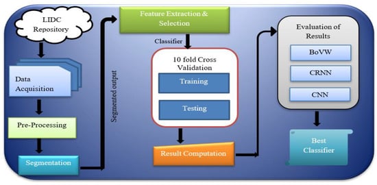
Figure 1.
Block diagram of the cancer detection method.
For detecting cancer, various techniques are being proposed and used. Ami George [9] proposes a technique to denoise the medical image using transformed wavelets. Denoising is done by considering different wavelets of hard threshold, and one related to that named PSNR image metric was tried but did not provide a satisfying result. Jin et al. [10] aim at the CNN (Convolution Neural Network) system in their CAD framework, providing an exactness of 84.6%, a sensitivity of 82.5%, and a specificity of 86.7%. The main plus point of this framework is that during the extraction stage, it uses the filter in ROI (Region of Interest), thereby diminishing the expense of the remaining steps. Other than that, the other problem is diminishing execution cost, thereby producing uneven exactness. Sarah et al. [11] aim to use a robust lung algorithm to segment lungs. A median filter and fuzzy thresholding are utilised for pre-processing of images. This method does not create over and under-segmentation problems because it is a robust segmentation method.
Lilik et al. [12] aim to improve intensity using image processing techniques such as grayscale, binary, median filters, and histogram. Grayscale conversion occurs when an RGB image is converted to a grayscale image, which is the same as converting an image to binary form. The median filter is used to reduce noise, and the histogram is used to improve image quality for better understanding. Malarvel et al. [13] aim for segmentation as an automatic seed choice format in ROI (Region of Interest) that has uneven backgrounds in radiographic images. Zhang et al. [14] propose a method which aims at segmentation by extricating the feature of an image using a tensor that is a nonlinear structure, and then use the Grabcut strategy, thereby producing exact impact.
Ajin et al. [15] aim at three things: the removing, choosing, and classifying features. Other strategic methods include Linear Ternary Co-occurrence Pattern, histogram feature determination, and Hybrid kernel SVM classifier, which are used for extracting features, choosing the features, and also grouping these features. Another strategy proposed by Selin et al. [16] aims to fragment, in image processing, the lung tumor in CT images, and some other features are also used to reduce the noise in images, followed by separating the tumor from a picture by portioning the image in a later stage. Threshold will select automatically based on gray level intensities in each image. Another method proposed by Wang et al. [17] provides less cycle process aims in improving sequential cuts in the segmentation of lungs through nearby cuts in data. Shengchao et al. [18] aim to improve GrabCut for lung parenchyma division. This method can choose a bounding box that can relate CT images of the lung parenchyma, using the Grabcut strategy to precisely portion those images. When choosing the bounding box, it conquers standard GrabCut calculation and is also harsh regarding noise.
Ganesh et al. [19] aim for a clear segmentation to improve the CAD framework and examine those images. However, it provides a confused state regarding juxtapleural nodules and pulmonary vessels. The mentioned method contains three stages of lung field segmenting, detecting dominant points from concave and convex points using curvature information. Finally, a boundary correction is required to repair the boundary.
Piotr et al. [20] describe the automated investigation of medical images, where calculation fully depends on a level set which unites a Chan–Vese segmentation with active dense estimation. This brings out two key points: first, it allows surface-based division methods, and second, it consolidates earlier learning into a scientifically proven way. Narain et al. [21] bring out another method to use image processing in the Lung Cancer discovery model. It contains three phases: pre-processing, feature extraction, and classification. Along with that, by using an SVM classifier, it can predict if the lung is normal or abnormal. LOOP (Local Optimal Oriented Pattern) separates texture features, and K-fold comes in handy for characterising. Later, different binary designs such as LBP (Local Binary Pattern), LBC (Local Binary Count), and LDP (Local Directional Pattern) are employed, which contrasts the results with the outcome.
Ezhil et al. [22] provide an active contour model using the level set capacity for the segmentation of lungs. CT (Computed Tomography) offers so much ease in investigating images. Here, it mainly offers us two great strategies, Selective Binary and Gaussian filtering new Signed Pressure Force (SBGF-new SPF) for CT lung image segmentation, which describes the difference in the external boundary of the lung and the stops happening at blurry boundaries. The calculation time and the segmented lung show the upside version of the proposed system. Gupta et al. [23] put forward another strategy to investigate medical images, thereby helping medical specialists diagnose the illness and provide worthy medications and counteracts. The task is to recognise and classify them as solid and maladies such as Chronic Obstructive Pulmonary Disease (COPD) and Fibrosis. During the initial period for determination of features from a pool of portioned lungs, the work concentrates on using Gray Level Co-occurrence Matrix (GLCM), Zernike’s minutes, Gabor features, and Tamura texture features. For feature selection as the second aim, three algorithms proposed involving the Improvised Crow Search Algorithm (ICSA), Improvised Grey Wolf Algorithm (IGWA), and Improvised Cuttlefish Algorithm (ICFA) are employed, thereby selecting features from a large set of pools that are extracted from the image to improve accuracy and reduce cost. As the final step, it uses four classifiers from ML, such as k-Nearest Neighbor (KNN), Support Vector Machine (SVM), Random Forest Classifier, and Decision Tree Classifier applied to each feature subset.
An earlier generation of medical imaging is hard to analyse manually, so the consequences that can occur while segmenting fully rely on exactitude and convergence time [24]. As a result, there is a necessity to develop new and more accurate methods for image segmentation [25]. CT is mainly used to diagnose lung cancer because it is still the most cost-effective type of medical imaging. Recent work in algorithms such as k-means clustering, k-median clustering, particle swarm optimisation, inertia-weighted particle swarm optimisation, and Guaranteed Convergence Particle Swarm Optimization (GCPSO) have been used to extract tumors from lung images and analyse them. Medical images frequently require pre-processing before being subjected to statistical analysis [26,27,28]. Thereby, latest technologies such as ML take AI in hand to produce advanced models for even more accurate results as these models are used to learn from previous data.
2. Materials and Methods
In the proposed solution in this research, the first step was running image pre-processing for identifying particles. That was briefly done via intensity measurement. Afterwards, the pre-processed image was segmented using a standard segmentation technique followed by extraction and selection of features. Some texture features were extracted during feature extraction using the Approximate Bayesian Computation (ABC) parameter, the GLCM method, and the Factor of Safety (FOS) parameter. It was then followed by the classification process, which includes benign and malignant tumors, considering the CT scanned images. A few extracted features were used to train the classifier. The corresponding trained classification model was created with the model evaluation and obtained improved detection and classification accuracy, specificity, and sensitivity. Figure 2 shows the basic framework for the proposed system.

Figure 2.
Framework for the detection of Lung cancer for a CAD System [28].
2.1. Image Acquisition
All the images used in this research are also accessible in the database, with the pivotal point of view. Here, the framework size is (256 × 256) or (512 × 512) and 16 bits for every pixel. Lung Image Database Consortium (LIDC) is where the JPEG format of lung images is available. For research purposes of radiologists, they can easily access that database through Cancer Imaging Archive (CIA) [29]. Some samples from the databases are shown in Figure 3. The proposed system data set consists of images of 290 patients, of which 250 patient datasets are used for training the classifier, and the remaining 40 patient datasets are used for validation. The data set obtained is of DICOM format and is converted to 512 × 512 by pre-processing method without data loss for further partitioning and refinement purposes. Table 1 summarizes the dataset used, and Table 2 shows the scanner difference.
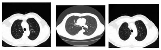
Figure 3.
CT image of lungs from the dataset: LIDC in the different sagittal planes.

Table 1.
Overview of the Dataset used.
Table 2.
Dataset statistics in terms of different scanner.
2.2. Pre-Processing
In the research process, the CT images were pre-handled at the lowest level of abstraction to improve each image’s quality. The operation to detect tumors was image enhancements after that analysed and preceded the noise reduction, image enhancement (via Gabor filter), and contrast adjustment (with the modified color-based histogram equalisation).
2.2.1. Gabor Filter
After Dennis Gabor, the name of Gabor filter came into existence; the filter can be used for texture analysis purposes. When the Gaussian and harmonic function is multiplied, we gain an impulsive response of that filter. It mainly analyses if there is any specific frequency in the specific direction of an image [30]. That filter is the most suitable solution for texture representation and discrimination of images in the spatial domain. The Figure 4a,b shows the CT lung images and the Gabor filter pre-processed images in this research work, respectively.

Figure 4.
Output of the pre-processed images: (a) the lung CT images (b) Gabor filter enhancement.
2.2.2. Modified Color-Based Histogram Equalisation
The contrast adjustment of the image was made by histogram equalisation. As a result of such adjustment, a high level of contrast may occur in a particular region. In order to overcome that, the Modified Color Histogram Equalisation was employed in this research. That includes limiting the amplitude of pixel intensities [31]. The transformation function slope and the Cumulative Distribution Function (CDF) are proportionate in this proposed system. The histogram was clipped, and the amplification was limited before computing the CDF. As a result, the CDF and transformation function slopes were reduced. The clip limit [32] is the value at which the histogram is clipped and consequently depends on the size of the neighboring region. Figure 5 shows the applied color-based histogram on the input image (pre-processed).
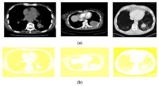
Figure 5.
Output of the pre-processed images: (a) The original input images (b) corresponding results of modified color-based histogram equalization.
A Cumulative Distribution Function (CDF) is provided as follows:
The output intensity of histogram equalisation is provided as
where and indicate the maximum permissible intensity, respectively, is the input intensity, and is the output intensity. () indicates the input intensity of CDF. Tumor pixel usually becomes white during the foreground region and color for the background region. The image contrast is gained via the following equation [33,34]:
where fm is the foreground region’s mean color level, and bm is the background region’s mean color level.
The CII method was used in research to measure the image enhancement algorithm efficiency. By dividing the ratio of the contrast of the (enhanced) output image with respect to the contrast of the input image, we gain CII,
where corresponds to the processed image contrast, and defines the input image contrast.
2.3. Segmentation: GCPSO Method
The Guaranteed Convergence Particle Swarm Optimization (GCPSO) algorithm is based on a new Particle Swarm Optimization (PSO) algorithm-based optimisation solution, which considers that each particle is evaluated according to the suitable location in the current region [16,35]. GCPSO was applied for segmentation purposes. At this point, the parameters for the “NC” and “MC” thresholds were defined empirically. During some iterations, gaining a better value in high-dimension search space is difficult. So, the values that are being suggested are “NC” = 15 and “MC” = 5, respectively. For the GCPSO, different phases are included to improve the solution process. In some comparative studies, the GCPSO has demonstrated remarkable progress in searching within a minimum space with only a small number of particles [36]. In this sense, GCPSO was used to enhance the research segmentation results. Figure 6 represents the algorithm steps and the obtained images after implementation using the GCPSO, given in Algorithm 1.
| Algorithm 1. GCPSO |
Initialisation
|

Figure 6.
Segmentation results after applying the GCPSO algorithm.
2.4. Feature Extraction
Feature Extraction is a technique for minimising the dimensions in raw data so that it can be processed more easily and organised into manageable classes. Massive volumes of data are characterised by many variables that require computer resources to process and provide results. Feature Extraction strategies simplify data while guaranteeing that no information is lost. These methods are responsible for selecting and merging features to reduce the amount of data. Table 3 lists numerous feature extraction approaches and the features that should be considered for each technique. The extraction process for the feature was done by automatically identifying the lung lesions. Three main characteristics of feature extraction processes have been, respectively, ABC parameter [37], FOS parameter, and GLCM features [38]:
Table 3.
Extracted feature parameters for ABC, GLCM and FOS features.
2.4.1. ABC Parameter
ABC parameter is used to describe border structure, lesion diameter, and asymmetry as follows:
- (i)
- Asymmetry Index:
- (ii)
- Border Structure irregularity: calculated by density index, fractal dimension index, edge deflection, and gray transition.
- a.
- Density Index:
- b.
- Fractal dimension Index:where and
- c.
- Edge deflection:
- d.
- Gray transition: calculates gradient magnitude and direction of an image.
- (iii)
- Diameter: used to calculate less gradient length in terms of nanometer scale.
2.4.2. GLCM Features
This method calculates the frequency at which pixel pairs arrive with the specified value and the amount of time to characterise an image’s texture. It often follows a gray co-matrix model, and statistical features are extracted based on the number of occurrences [38]. The equation for texture features used in this GLCM method is provided below:
2.4.3. Statistical Features
Through the statistical analysis, statistical features are identified [39]. The analysis refers to the most frequently occurring number from the number set, and these features can be easily identified when compared with other structural feature extraction methods [40]. Statistical features used in our proposed system are provided below:
Figure 6 illustrates features selected for the CRNN classifier in this study. Here, 13 elements were selected and introduced as the inputs to the CRNN model. The proposed CRNN architecture included four hidden layers and one output layer with 13 selected features as the input data. To decrease the number of features that have been selected and have less training time, the feature selection process, as referred to in [41], was performed accordingly. At this point, we mapped five characteristics from the CRNN classifier: efficiency, train state, histogram error, confusion, and operating characteristics of the receiver. Table 3 shows the extracted parameter values after applying the ABC, GLCM, and FOS feature extraction methods. This extracted feature from the original feature set helped to minimise the time for training for the classifier and increasing classifier efficiency in finding out the malignant and benign tumors.
2.5. Classification
2.5.1. BoVW Classifier
Bag of visual words (BoVW) is an extension of the NLP algorithm which follows the supervised learning model. The classifier aims to reduce time consumption by automatically selecting the features accompanying the classification process. It is a commonly used solution, apart from the widely-known CNN [42]. BoVW has been developed to obtain a comprehensive language which can better explain the image in terms of extrapolated features. BoVW employs the Computer Vision Toolbox TM functions to define image categories by constructing a bag of visual words. The proposed approach generates a histogram of the image by considering the frequency of visual words. After that, the histogram is utilised for training a classifier for image categories. The procedures below show the to set up process of the target images, generating a bag of visual words, and then training and application of an image classification classifier [43]. The BoVW is broken down into four simple steps: (1) analysis of the image qualities of a given label; (2) clustering used to create visual vocabulary, which is preceded by frequency analysis, (3) vocabulary classification of the produced samples, (4) determination of the most appropriate class for the image query. The algorithm for the bag of visual words classifiers is as follows:
Step 1: Image Sets created based on Category.
Step 2: BoVW Features is set up.
Step 3: CRNN Classifier is trained with BoVW features.
Considering the BoVW, the images are split into training and test subjects. Before that, a bag of features is created by extracting character descriptors from representative images for each category. The image is generally encoded from the training collection in the visual words system bag so that the properties from the image are taken [44].
2.5.2. CRNN Classifier
In this research, a Convolutional Recurrent Neural Network (CRNN) was also used for classification purposes. The CRNN briefly uses the pipeline architecture of neural networks, where CNN plays the first part, and an RNN is employed in the next part. Figure 7 illustrates the basic architecture of a typical CRNN model. In the context of the research done here, the input for the CRNN network is a nano lung image. Additionally, among the four layers in the CRNN architecture, two Convolutional layers were used to learn the input image. For training data without overfitting, matched filters and the dropout layer [16,45] are good options for use. In addition, the fourth convolution layer, is considered, inorder to downsample the output of the previous layer max-pooling.

Figure 7.
Basic architecture of CRNN.
It is possible to explain the exact mechanism inside the modeled CRNN as follows: The CRNN Convolutional layers form a neuron grid in rectangular mode. The neuron receives its previous input layer rectangular grid; for each neuron, the weight for this Convolutional layer will be the same. The size of the Convolutional layer here is calculated based on the 2D convolution filter size and the number [46]. Output from the Convolutional layer is transferred to the dropout layer and is concatenated by monitoring the number of neurons from the previous layer. The Max-pooling layer, the fourth layer that accepts small rectangular blocks from the previous Convolutional layer, extracts maximum output by reducing the error [47,48]. The RNN part consists of LSTM and Softmax. For temporal modeling, subsequent layers of learned filters are fed by LSTM. The layer composed of LSTM cells is called as the layer LSTM. As per the name, it memorises every step of the previous action and adds along with its current state [49]. The weight parameters in the LSTM layer are shared over time steps. Finally, Softmax activation is the last layer to derive model output values.
2.5.3. Convolution Neural Network (CNN)
A Convolution Neural Network (CNN) is a type of multilayer neural network that, like a standard multilayer neural network, comprises one or more convolution layers followed by one or more fully connected layers. CNN was founded in 1960 and included concepts such as local perception, sharing weights, and spatial and temporal sampling. Local perception can detect certain local properties of the data for basic features of visual animals, such as an angle and an arc in a picture [14]. It is a new efficient identification method that is gaining much attention. CNNs are easier to train and have smaller parameters than fully connected networks with the same number of hidden units.
The Convolution Neural Network architecture [50,51] commonly uses convolution and pool layers. The pooling layer’s favorite activity perplexes a specific location’s peculiarities. Because some location features are not required, the other features and relative positions are all required. The pooling layer has two operations: maximum pooling and mean pooling. Mean pooling is used to obtain the average neighborhood inside the feature points, whereas max pooling calculates the largest neighborhood. The two main sources of feature extraction error are the neighborhood size limitation induced by the estimated variance and the convolution layer parameter estimated error caused by the mean deviation. The first error can be minimised using mean pooling, which retains more image background information. Max pooling can help to reduce the second error by retaining more texture information.
The architecture of the CNN employed in this study is depicted in Figure 1. Each layer contains several maps; each map contains numerous neural units, all of which share the same convolution kernel (i.e., weight), and each convolution kernel represents a feature, such as access to the edge of visual features. The detailed architecture of CNN is depicted in further depth in Figure 8, and the parameters used in CNN architecture are in Table 4. The distortion tolerance of the input data (image data) is very high. The multiscale convolution image feature is created by adjusting the convolution kernel size and parameter; information from various angles is generated in the feature space.

Figure 8.
Basic Architecture of CNN.
Table 4.
Parameters used in CNN architecture.
3. Results
There was a great requirement for sophisticated hardware and software setup to perform the desired lung tumor diagnosis approach in this research. As it is known, the performance parameters such as computation time depend on the employed hardware and software infrastructure. Therefore, a wise selection of available hardware and software was made in this research. At this point, a Graphical User Interface (GUI) was thought to ensure better interactivity with visual indicators and icons (rather than dealing with just the code). Running and debugging the code is a tedious process [51]. GUI here provided some buttons to navigate and execute every function in the MATLAB environment. The designed GUI in this research supported displaying input images, segmented images, extracted features, and classification outputs. Remarkably, the GUI can easily obtain classifiers’ testing and training performance. The GUI was developed using an inbuilt MATLAB tool called GUI Development Environment (GUIDE) [50].
3.1. Software and Hardware Set-Up
The sample images were taken from the LIDC database, and the dataset was available via NCI. This dataset comprises 86 benign and 86 malignant images in DICOM (Digital Imaging and Communications in Medicine) format. Dimensions of the entire CT image dataset are 512 × 512 pixels, with a 12-bit bit depth. MATLAB (2016) and the Microsoft Windows 8.1 operating system were chosen in this research to ensure a stable computing experience. On the other hand, Intel core i3 (model number 4030U) was used as the Central Processing Unit (CPU) with a clock speed of 1.9 GH. The CPU has a 64-bit computational capacity and Intel data protection technology. The memory used in the system had a size of 4 gigabytes, and the cache memory was 3 megabytes [52]. That processor provides increased computing speed and is optimum for running MATLAB software.
3.2. Performance Measures
Performance parameter numeric description is vital in analysing the information based on the individual group. It provides a clear idea regarding the outcomes and results. Equations of the performance measure used in this research for evaluating the proposed system are provided below:
The step-by-step segmented output and classification procedure for the proposed method is shown in Figure 9 and Figure 10 (for the benign and malignant dataset). It is an image-calculated tumor area based on the nano technique, and the status of the tumor area of the malignant sample is shown in Table 5.
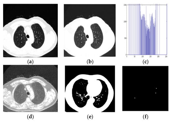
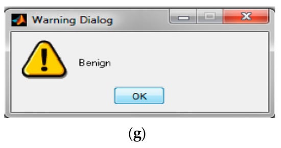
Figure 9.
Detection of Benign Sample. (a) Input CT Image, (b) Pre-processed output, (c) Histogram Equalised Image Plot, (d) Histogram Equalised Image, (e,f) Segmentation image, (g) Classification result.

Figure 10.
Detection of malignant Sample. (a) Input CT Image, (b) Pre-processed Output image, (c) Histogram Equalised Image Plot, (d) Histogram Equalised Image, (e,f) Segmentation image, (g) Classification result.
Table 5.
Parameter calculation of nodules.
Ultimately, the Bag of Visual Word classifier’s classification results showed whether the picture was benign or malignant. Figure 11a,b shows the Bag of Visual Word results plot. This classifier shows the outcome of detection of benign classification in Figure 9 and malignancy classification in Figure 10.
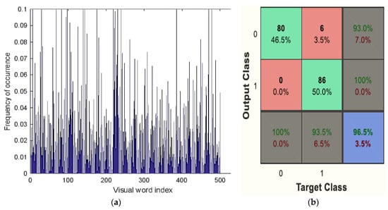
Figure 11.
(a) Visual vocabulary of BoVW classifier, (b) Confusion matrix of BoVW classifier.
The RNN classifier model in the basic NN tool of the MATLAB environment is shown in Figure 12. The overall performance of the recurrent neural system and the performance evaluation of the RNN in terms of receiver operating characteristics, error histogram, and train state are plotted in Figure 13. The performance of each of the instructions given, evaluation part, and test sets are also shown in Figure 14. The mean squared error and the log scale for output calculation are associated with the results. It shrinks due to network training. The matrix of ambiguity provides the correct and incorrect classification. In addition, 0 to 1 is a range of outputs representing benign or malignant images/patients.

Figure 12.
The RNN model as designed in the NN tool MATLAB.

Figure 13.
Overall performance of the recurrent neural system.

Figure 14.
The performance of the given instructions, evaluation, and test sets.
In the CNN, a ResNet-50 model consisted of five stages, each with a block of identity and a convolution layer employed accordingly. Every block of the convolution had three layers of convolution, and each block of identity had three layers. The ResNet-50 had trainable parameters of over 23 million.
The obtained accuracy after optimisation was 98.5%. Table 6 analyses performance parameters for the BoVW and CRNN classifiers. The parameters considered here are accuracy, sensitivity, specificity, precision, PSNR and MSE values. For the BoVW classifier, accuracy was 96.5%, sensitivity was 93%, specificity was 100%, precision was 93.5%, PSNR value was 42.278, and the MSE was 3.474. For the CRNN classifier, accuracy was 98.5%, sensitivity was 95%, specificity was 100%, precision was 95.5%, PSNR was 69.154, and the MSE was 2.193. From Table 6, it is clear that CRNN provided the best output performance in terms of accuracy and precision. Table 7 shows the error and accuracy comparison regarding different classifiers. Figure 15 shows (a) the Performance Measure of the classifier and (b) the Performance Graph of the classifier.
Table 6.
Analysis of performance parameters.
Table 7.
Accuracy and Error Comparison of Classifiers.
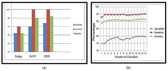
Figure 15.
(a) Performance Measure of the classifier, (b) Performance Graph of the classifier.
Compared to other methods, the proposed nano-based CRNN classifier provides 98.5% accuracy, which is greater than other techniques (Table 8). The proposed technique effectively smooths the image and accurately determines the minute nodules. Finally, the technique accurately classifies the image, whether benign or malignant.
Table 8.
Comparison with existing lung tumor detection methods.
4. Conclusions
This paper presents us with a great advanced visual of diagnosing lung cancer in the early stages. In detail, the solution has been designed based on a computer-aided diagnostic (CAD) approach using computed tomography (CT) images. We briefly presented a framework for creating an early model of cancer diagnosis using CAD CT image processing. The attributes of the research included: (1) increased cancer nodule detection accuracy, (2) classifying suspected lung cancer as malignant or benign, and (3) removing noise-causing false detection rate using a nanotechnology-based detection method. Analysis of the different existing classifiers was done to properly diagnose lung cancer. CT Images of lung malignancy were taken, and pre-processing methods were used to remove noise and enhance the image. To separate the cancerous area of the healthy lung, the GCPSO-based segmentation technique was used along with a nano-measuring instrument, which is useful for detecting the tumor’s location at a nano-scale. Depending on the characteristic, features of segmented regions are extracted, and by using the classifier Bag of Visual Words and the CRNN, the classification/diagnosis was made accordingly.
In the future, we may extend our current model to determine whether or not the patient has cancer and the precise location of the cancerous nodules. Watershed segmentation can be used for the initial lung segmentation in future. Other areas for improvement include expanding the network and performing more extensive hyperparameter tuning. In addition, we saved our model parameters at the highest accuracy, but we could have saved them at a lower metric, such as F1. Our models can also be extended to 3D images for other cancers.
Author Contributions
Conceptualisation, A.S.U.; Data curation, A.S.U. and A.A.; Formal analysis, A.S.U., A.A. and F.R.P.P.; Funding acquisition, F.R.P.P.; Investigation, A.S.U., A.A. and F.R.P.P.; Methodology, A.S.U.; Project administration, A.S.U.; Resources, A.S.U., A.A., F.R.P.P. and D.S.; Software, A.S.U.; Supervision, A.S.U.; Validation, A.S.U., A.A., F.R.P.P. and D.S.; Visualization, A.S.U., A.A., F.R.P.P. and D.S.; Writing—original draft, A.S.U., A.A., F.R.P.P. and D.S.; Writing—review and editing, A.S.U., A.A., F.R.P.P. and D.S. All authors have read and agreed to the published version of the manuscript.
Funding
This research has been funded by The Deanship of Scientific Research, King Faisal University, Saudi Arabia, with grant Number (GRANT2221).
Data Availability Statement
The study did not report any data.
Acknowledgments
We deeply acknowledge The Deanship of Scientific Research, King Faisal University, Saudi Arabia.
Conflicts of Interest
The authors declare no conflict of interest.
References
- Choi, W.J.; Choi, T.S. Automated Pulmonary Nodule Detection System in Computed Tomography Images: A Hierarchical Block Classification Approach. Entropy 2013, 15, 507–523. [Google Scholar] [CrossRef]
- Trial Summary—Learn—NLST—The Cancer Data Access System. Available online: https://biometry.nci.nih.gov/cdas/learn/nlst/trial-summary/ (accessed on 7 January 2022).
- National Lung Screening Trial Research Team. Reduced Lung-Cancer Mortality with Low-Dose Computed Tomographic Screening. N. Engl. J. Med. 2011, 365, 395–409. [Google Scholar] [CrossRef] [PubMed]
- Wang, Z.; Xin, J.; Sun, P.; Lin, Z.; Yao, Z.; Gao, X. Improved lung nodule diagnosis accuracy using lung CT images with uncertain class. Comput. Methods Programs Biomed. 2018, 162, 197–209. [Google Scholar] [CrossRef] [PubMed]
- Bray, F.; Ferlay, J.; Soerjomataram, I.; Siegel, R.L.; Torre, L.A.; Jemal, A. Global cancer statistics 2018: GLOBOCAN estimates of incidence and mortality worldwide for 36 cancers in 185 countries. CA Cancer J. Clin. 2018, 68, 394–424. [Google Scholar] [CrossRef]
- Torre, L.A.; Siegel, R.L.; Jemal, A. Lung Cancer Statistics; Springer: Berlin/Heidelberg, Germany, 2016; pp. 1–19. [Google Scholar]
- Avinash, S.; Manjunath, K.; Senthil Kumar, S. An improved image processing analysis for the detection of lung cancer using Gabor filters and watershed segmentation technique. In Proceedings of the International Conference on Inventive Computation Technologies (ICICT), Coimbatore, India, 26–27 August 2016; Volume 3, pp. 1–6. [Google Scholar]
- Krishnamurthy, S.; Narasimhan, G.; Rengasamy, U. Lung nodule growth measurement and prediction using auto cluster seed K-means morphological segmentation and shape variance analysis. Int. J. Biomed. Eng. Technol. 2017, 24, 53. [Google Scholar] [CrossRef]
- George, A.; Logesh Kumar, S.; Manikandan, K.; Vijayalakshmi, C.; Renuga, R. Medical image using Denoising wavelet transform. Int. J. Circuit Theory Appl. 2016, 9, 3945–3949. [Google Scholar]
- Jin, X.; Zhang, Y.; Jin, Q. Pulmonary Nodule Detection Based on CT Images Using Convolution Neural Network. In Proceedings of the International Symposium on Computational Intelligence And Design (ISCID), Hangzhou, China, 10–11 December 2016. [Google Scholar]
- Soltaninejad, S.; Tajeripour, F. Robust Lung segmentation combining Adaptive concave hull with active contours. In Proceedings of the 11th Intelligent Systems Conference (ICIS), Budapest, Hungary, 9–12 October 2016; p. 69. [Google Scholar]
- Anifah, L.; Haryanto; Harimurti, R.; Permatasari, Z.; Rusimamto, P.W.; Muhamad, A.R. Cancer Lungs Detection on CT Scan Image Using Artificial Neural Network Backpropagation Based Gray Level Co-occurrence Matrices Feature. In Proceedings of the 2017 International Conference on Advanced Computer Science and Information Systems (ICACSIS), Jakarta, Indonesia, 28–29 October 2017; Volume 47. [Google Scholar]
- Malarvel, M.; Sethumadhavan, G.; Bhagi, P.C.R.; Thangavel, S.; Krishnan, A. Region growing based segmentation with automatic seed selection using threshold techniques on X-radiography images. In Proceedings of the 2016 IEEE International Conference on Computational Intelligence and Computing Research (ICCIC), Chennai, India, 15–17 December 2016; pp. 1–4. [Google Scholar]
- Yong, Z.; Jiazheng, Y.; Hongzhe, L.; Qing, L. GrabCut image segmentation algorithm based on structure tensor. J. China Univ. Posts Telecommun. 2017, 24, 38–47. [Google Scholar] [CrossRef]
- Ajin, M.; Mredhula, L.B. Diagnosis Of Interstitial Lung Disease By Pattern Classification. In Proceedings of the International Conference on Advances in Computing & Communications, Kochi, India, 22–24 August 2017; pp. 22–24. [Google Scholar]
- Uzelaltinbulat, S.; Ugur, B. Lung tumor segmentation algorithm. Procedia Comput. Sci. 2017, 120, 140–147. [Google Scholar] [CrossRef]
- Wang, L.A.; Bray, F.; Siegel, R.L.; Ferlay, J.; Lortet-Tieulent, J.; Jemal, A.C.A. Automatic Approach for Lung Segmentation with Juxta-Pleural Nodules from Thoracic CT Based on Contour Tracing and Correction. Comput. Math. Methods Med. 2016, 65, 87–108. [Google Scholar] [CrossRef]
- Zhang, S.; Zhao, Y.; Bai, P. Object Localization improved Grabcut for Lung Parenchyma Segmentation. In Proceedings of the 8th International Congress of Information and Communication Technology, Xiamen, China, 27–28 January 2018; Volume 131, pp. 1311–1317. [Google Scholar]
- Singadkar, G.; Mahajan, A.; Thakur, M.; Talbar, S. An Automatic lung segmentation for the inclusion of juxtapleural nodules and pulmonary vessels using curvature based border correction. J. King Saud Univ.—Comput. Inf. Sci. 2018, 77, 975–987. [Google Scholar] [CrossRef]
- Swierczynskia, P.; Papiez, B.W.; Schnabelb, J.A.; Macdonald, C. A level-set approach to joint image segmentation and registration with application to CT lung imaging. Comput. Med. Imaging Graph. 2018, 65, 58–68. [Google Scholar] [CrossRef] [PubMed]
- Narain Ponraj, D.; Christy, E.; Aneesha, G.; Susmitha, G.; Sharu, M. Analysis of LBP and LOOP Based Textural Feature Extraction for the Classification of CT Lung Images. In Proceedings of the Fourth International Conference on Devices, Circuits and Systems, Coimbatore, India, 16–17 March 2018; IEEE: Piscataway, NJ, USA, 2018. [Google Scholar]
- Nithila, E.E.; Kumar, S.S. Segmentation of lung from CT using various active contour models. Biomed. Signal Process. Control 2019, 47, 57–62. [Google Scholar] [CrossRef]
- Gupta, N.; Gupta, D.; Khanna, A.; Rebouças Filho, P.P. Evolutionary Algorithms for Automatic Lung Disease Detection. J. Meas. 2019, 140, 42–117. [Google Scholar] [CrossRef]
- Abdel-Massieh, N.H.; Hadhoud, M.M.; Moustafa, K.A. A fully automatic and efficient technique for liver segmentation from abdominal CT images. In Proceedings of the International Conference on Informatics and Systems, Cairo, Egypt, 28–30 March 2010; pp. 1–8. [Google Scholar]
- Armato, S.; Hadjiiski, L.; Tourassi, G.; Drukker, K.; Giger, M.; Li, F.; Redmond, G.; Farahani, K.; Kirby, J.; Clarke, L. Spie-aapm-nci lung nodule classification challenge dataset. Cancer Imaging Arch. 2015, 2, 020103. [Google Scholar] [CrossRef]
- Mathews, A.B.; Jeyakumar, M.K. Quantitative Evaluation of Lung Tumor Detection Applied to Axial MR Images. Int. J. Electr. Electron. Comput. Sci. Eng. 2019, 6, 17–19. [Google Scholar]
- Thiyagarajan, A.; Pandurangan, U. Comparative analysis of classifier Performance on MR brain images. Int. Arab. J. Inf. Technol. 2015, 12, 772–779. [Google Scholar]
- Tisdall, D.; Atkins, M.S. MRI Denoising via Phase Error Estimation; International Society for Optics and Photonics: Washington, DC, USA, 2005; pp. 646–655. [Google Scholar]
- Saba, T. Recent advancement in cancer detection using machine learning: Systematic survey of decades, comparisons and challenges. J. Infect. Public Health 2020, 13, 1274–1289. [Google Scholar] [CrossRef]
- Armato, S.G., III; McLennan, G.; Bidaut, L.; McNitt-Gray, M.F.; Meyer, C.R.; Reeves, A.P.; Zhao, B.; Aberle, D.R.; Henschke, C.I.; Hoffman, E.A.; et al. Data From LIDC-IDRI [Data set]. Cancer Imaging Arch. 2015. [Google Scholar] [CrossRef]
- Vovk, U.; Pernus, F.; Likar, B. A review of methods for correction of intensity inhomogeneity in MRI. IEEE Trans. Med. Imaging 2007, 26, 405–421. [Google Scholar] [CrossRef]
- Hitosugi, T.; Shimizu, A.; Tamura, M.; Kobatake, H. Development of a liver extraction method using a level set method and its performance evaluation. J. Comput. Aided Diagn. Med. Images 2003, 7, 1–9. [Google Scholar]
- Tajima, T.; Zhang, X.; Kitagawa, T.; Kanematsu, M.; Zhou, X.; Hara, T.; Fujita, H.; Yokoyama, R.; Kondo, H.; Hoshi, H. Computer-aided detection (CAD) of hepatocellular carcinoma on multiphase CT images. In Medical Imaging; SPIE: Washington, DC, USA, 2007. [Google Scholar]
- Asada, N.; Doi, K.; MacMahon, H.; Montner, S.M.; Giger, M.L.; Abe, C.; Wu, Y. Potential usefulness of an artificial neural network for differential diagnosis of interstitial lung disease: Pilot study. Radiology 1990, 177, 857–860. [Google Scholar] [CrossRef]
- Fujita, H.; Katafuchi, T.; Uehara, T.; Nishimura, T. Application of artificial neural network to computer-aided diagnosis of coronary artery disease in myocardial SPECT bull’s-eye images. J. Nucl. Med. 1992, 33, 272–276. [Google Scholar]
- Zhang, W.; Doi, K.; Giger, M.L.; Nishikawa, R.M.; Schmidt, R.A. An improved shiftinvariant artificial neural network for computerised detection of clustered microcalcifications in digital mammograms. Med. Phys. 1996, 23, 595–601. [Google Scholar] [CrossRef] [PubMed]
- Zhang, J.-P.; Li, Z.-W.; Yang, J. A parallel SVM training algorithm on the large-scale classification problems. In Proceedings of the International Conference on Machine Learning and Cybernetics, Guangzhou, China, 18–21 August 2005. [Google Scholar]
- Mathews, A.B.; Jeyakumar, M.K. Segmentation of Lung Images for Tumor Detection using Color Based k-means Clustering Algorithm. J. Int. Pharm. Res. 2019, 46, 191–197. [Google Scholar]
- Vijay, M. Detection of Lung Cancer Stages on CT scan Images by Using Various Image Processing Techniques. IOSR J. Comput. Eng. 2014, 16, 28–35. [Google Scholar]
- Goncalves, L.; Novo, J.; Campilho, A. Feature definition, analysis and selection for lung nodule classification in chest computerised tomography images. In Proceedings of the 2016 European Symposium on Artificial Neural Networks, Computational Intelligence and Machine Learning, Bruges, Belgium, 27–29 April 2016. [Google Scholar]
- Haralick, R.M.; Shanmugam, K.; Dinstein, I. Textural Features for Image Classification. IEEE Trans. Syst. 1973, 3, 610–621. [Google Scholar] [CrossRef]
- Dhawale, A.P.; Hirekhan, S.R. Real time image processing for biological applications through morphological operations using LabVIEW. Int. J. Eng. Res. Technol. IJERT 2014, 3, 1262–1265. [Google Scholar]
- Han, H.; Li, L.; Han, F.; Song, B.; Moore, W.; Liang, Z. Fast and adaptive detection of pulmonary nodules in thoracic CT images using a hierarchical vector quantisation scheme. IEEE J. Biomed. Health Inform. 2015, 19, 648–659. [Google Scholar] [CrossRef]
- Kuruvilla, J.; Gunavathi, K. Lung cancer classification using neural networks for CT images. Comput. Methods Programs Biomed. 2014, 113, 202–209. [Google Scholar] [CrossRef]
- Tiwari, A.K. Prediction of lung cancer using image processing techniques: Review. Adv. Comput. Intell. Int. J. ACII 2016, 3, 1–9. [Google Scholar] [CrossRef]
- Subhasri, P. Image Encryption using Advanced Multilevel Encryption. Glob. J. Eng. Sci. Res. 2019, 6, 519–524. [Google Scholar]
- Suzuk, K.; Armato, S.G., III; Li, F.; Sone, S.; Doi, K. Massive training artificial neural network (MTANN) for reduction of false positives in computerised detection of lung nodules in low-dose computed tomography. Med. Phys. 2003, 30, 1602–1617. [Google Scholar] [CrossRef] [PubMed]
- Javaid, M.; Javid, M.; Rehman, M.Z.U.; Shah, S.I.A. A novel approach to CAD system for the detection of lung nodules in CT images. Comput. Methods Programs Biomed. 2016, 135, 125–139. [Google Scholar] [CrossRef] [PubMed]
- Jiangdian, S.; Caiyun, Y.; Li, F. Lung lesion extraction using a toboggan based growing automatic segmentation approach. IEEE Trans. Med. Imaging 2015, 10, 1–16. [Google Scholar] [CrossRef] [PubMed]
- Gonzalez, R.C.; Woods, R.E.; Eddins, S.L. Digital Image Processing Using MATLAB; Gatesmark Publishing: Knoxville, TN, USA, 2004. [Google Scholar]
- Aswathy, S.U.; Abraham, A. A Review on State-of-the-Art Techniques for Image Segmentation and Classification for Brain MR Images. Curr. Med. Imaging 2022, 19, 243–270. [Google Scholar]
- Mathews, A.B.; Jeyakumar, M.K. Automatic Detection of Segmentation and Advanced Classification Algorithm. In Proceedings of the International Conference on Computing Methodologies and Communication, Erode, India, 11–13 March 2020; pp. 358–362. [Google Scholar]
Disclaimer/Publisher’s Note: The statements, opinions and data contained in all publications are solely those of the individual author(s) and contributor(s) and not of MDPI and/or the editor(s). MDPI and/or the editor(s) disclaim responsibility for any injury to people or property resulting from any ideas, methods, instructions or products referred to in the content. |
© 2022 by the authors. Licensee MDPI, Basel, Switzerland. This article is an open access article distributed under the terms and conditions of the Creative Commons Attribution (CC BY) license (https://creativecommons.org/licenses/by/4.0/).