
Application of the Multiverse Optimization Method to Solve the Optimal Power Flow Problem in Alternating Current Networks

 ,
,  ,
,  ,
,  and
and
Abstract
1. Introduction
1.1. General Context
1.2. State of the Art
1.3. Scope and Main Contributions
- A new solution methodology based on sequential programming to solve the OPF problem in AC networks that considers radial and mesh topologies.
- A robust statistical method that can be used to identify the solution methodology with the best balance of solution quality, processing times, and repeatability.
- An optimization method selected because it yields the best results in terms of solution quality, repeatability, and processing time to solve the OPF problem in AC networks with radial and mesh topologies.
- A new methodology that can be used to determine the optimal power level to be injected by each DG in order to reduce power losses and thus better use existing energy resources.
- A methodology with short processing times to solve the problem of sizing DGs in electrical networks.
1.4. Structure of the Paper
2. Mathematical Formulation
2.1. Objective Function
2.2. Set of Constraints
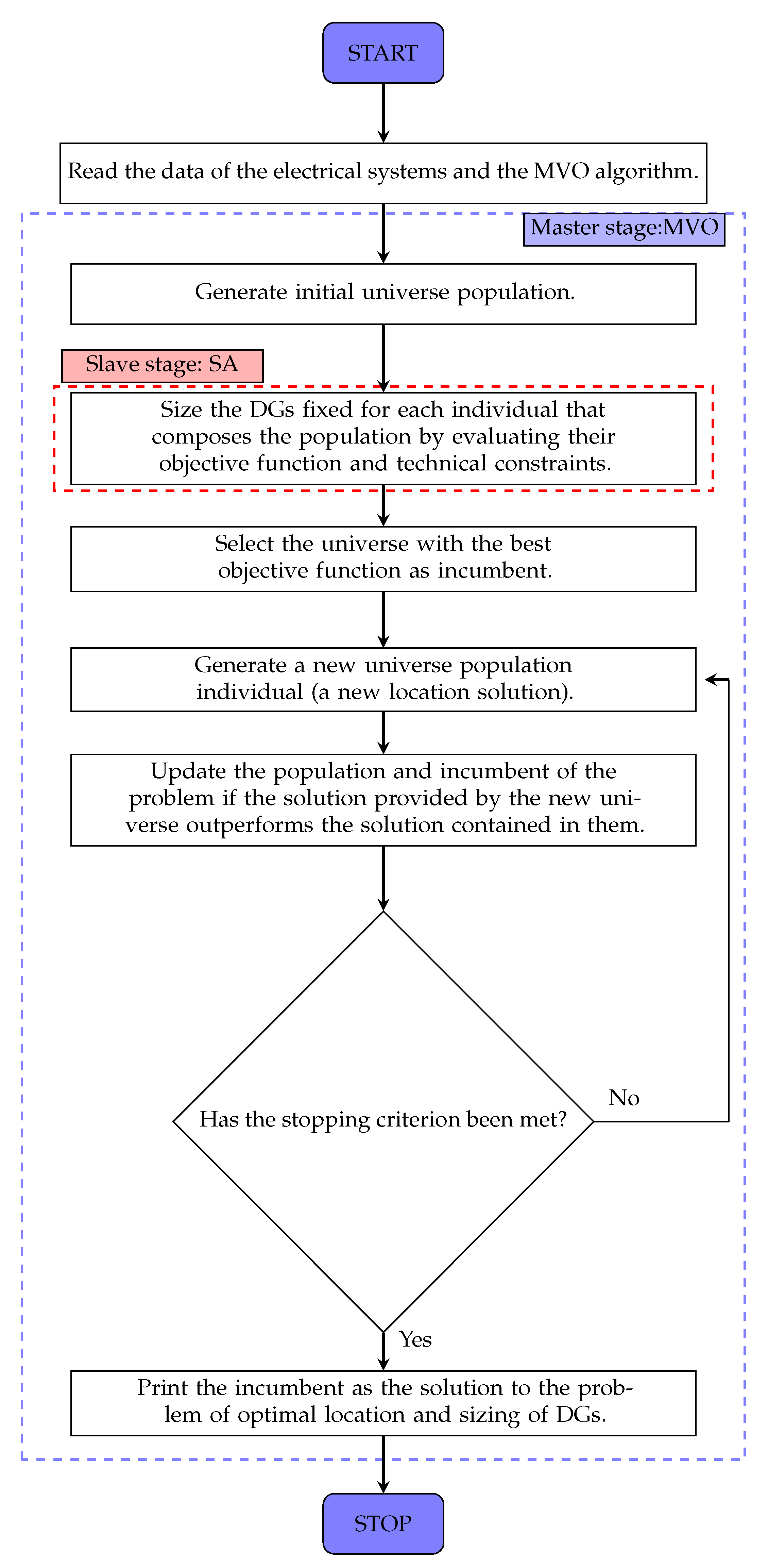
3. Proposed Solution Methodology
3.1. Master Stage: Multiverse Optimizer (MVO)
3.1.1. Generating the Initial Population
3.1.2. Calculating the Objective Function
3.1.3. Movement Strategy
- The higher the , the greater the probability of having a white hole.
- The lower the , the greater the probability of having a black hole.
- Universes with a high tend to send objects through white holes.
- Universes with a low tend to receive more objects through black holes.
- Any object in any universe can randomly move toward the best universe through wormholes, regardless of the .
3.1.4. Evolution of the Universes in the Iterative Process
| Algorithm 1. Proposed pseudocode of the roulette wheel to select universe k to transport element j to universe i. |
| 1:
function 2: 3: 4: 5: for do 6: if then 7: 8: break 9: end if 10: 11:end for |
3.1.5. Updating Universes Based on Wormholes
3.1.6. Stopping Criteria
- Maximum number of iterations: The iterative process will finish when the algorithm reaches the maximum number of iterations (L), which are controlled by counter l.
- Number of non-improvement iterations: The algorithm will stop when the incumbent solution is not updated after n consecutive iterations.
3.2. Slave Stage
4. Methods Used for Comparison Purposes
5. Test Scenarios and Considerations
5.1. Radial Test Systems
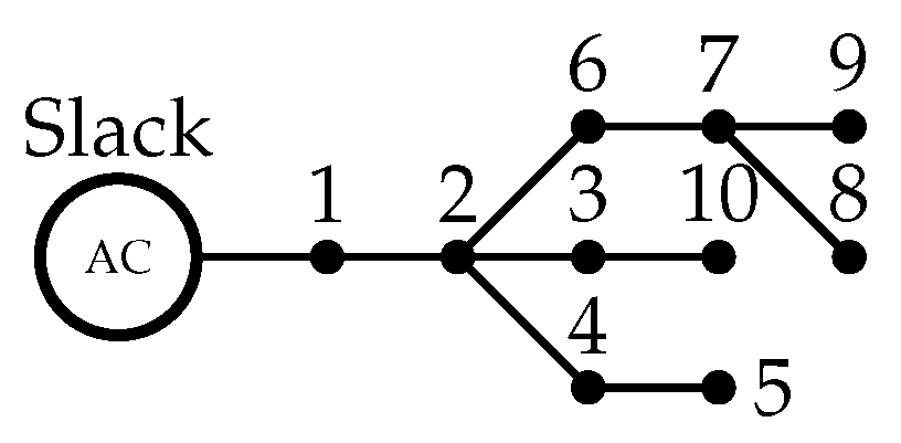
5.1.1. 10-Node Radial Test System
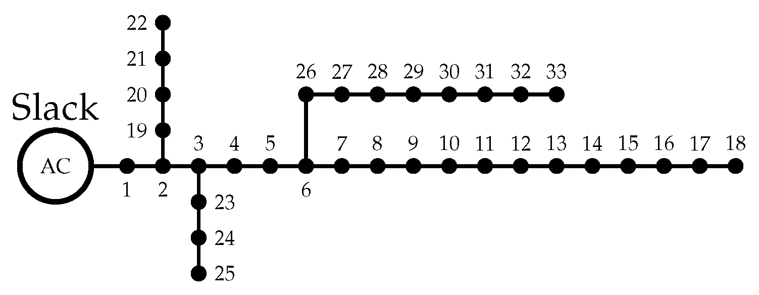
5.1.2. 33-Node Radial Test System
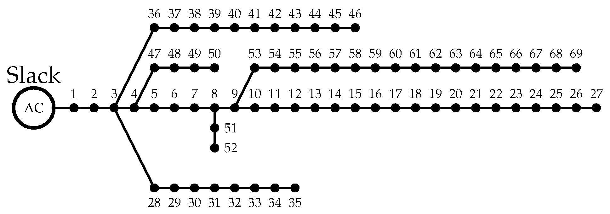
5.1.3. 69-Node Radial Test System
5.2. Mesh Test System
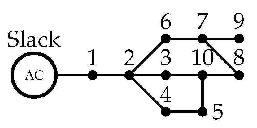
10-Node Mesh Test System
6. Simulations and Results
6.1. Results in the Radial Test Systems
6.1.1. 10-Node Radial Test System
6.1.2. 33-Node Radial Test System
6.1.3. 69-Node Radial Test System
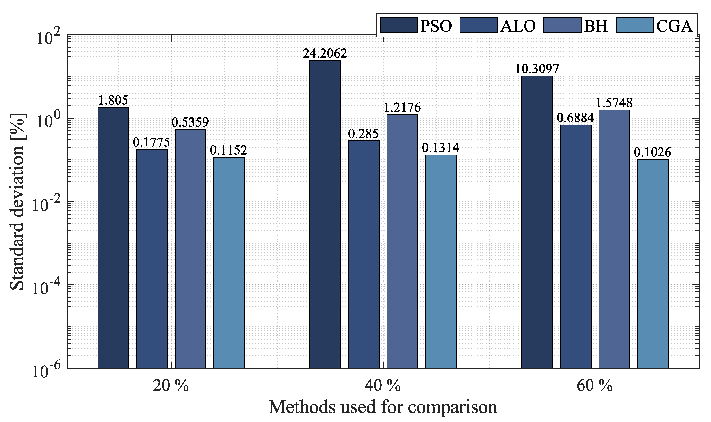
6.2. Results in the Mesh Test System
10-Node Mesh Test System
7. Conclusions
Author Contributions
Funding
Conflicts of Interest
References
- Gurven, M.; Walker, R. Energetic demand of multiple dependents and the evolution of slow human growth. Proc. R. Soc. B Biol. Sci. 2006, 273, 835–841. [Google Scholar] [CrossRef]
- Murillo, J.; Trejos, A.; OLAYA, P.C. Estudio del pronóstico de la demanda de energía eléctrica, utilizando modelos de series de tiempo. Sci. Tech. 2003, 3, 1–6. [Google Scholar] [CrossRef]
- Reiss, P.C.; White, M.W. Household electricity demand, revisited. Rev. Econ. Stud. 2005, 72, 853–883. [Google Scholar] [CrossRef]
- Halvorsen, R. Demand for electric energy in the United States. South. Econ. J. 1976, 42, 610–625. [Google Scholar] [CrossRef]
- Bull, S.R. Renewable energy today and tomorrow. Proc. IEEE 2001, 89, 1216–1226. [Google Scholar] [CrossRef]
- Machol, B.; Rizk, S. Economic value of US fossil fuel electricity health impacts. Environ. Int. 2013, 52, 75–80. [Google Scholar] [CrossRef]
- Zhang, N.; Zhou, P.; Choi, Y. Energy efficiency, CO2 emission performance and technology gaps in fossil fuel electricity generation in Korea: A meta-frontier non-radial directional distance functionanalysis. Energy Policy 2013, 56, 653–662. [Google Scholar] [CrossRef]
- Rosales Muñoz, A.A.; Grisales-Noreña, L.F.; Montano, J.; Montoya, O.D.; Giral-Ramírez, D.A. Optimal Power Dispatch of Distributed Generators in Direct Current Networks Using a Master–Slave Methodology That Combines the Salp Swarm Algorithm and the Successive Approximation Method. Electronics 2021, 10, 2837. [Google Scholar] [CrossRef]
- Rosales-Muñoz, A.A.; Grisales-Noreña, L.F.; Montano, J.; Montoya, O.D.; Perea-Moreno, A.J. Application of the Multiverse Optimization Method to Solve the Optimal Power Flow Problem in Direct Current Electrical Networks. Sustainability 2021, 13, 8703. [Google Scholar] [CrossRef]
- Grisales-Noreña, L.F.; Gonzalez Montoya, D.; Ramos-Paja, C.A. Optimal sizing and location of distributed generators based on PBIL and PSO techniques. Energies 2018, 11, 1018. [Google Scholar] [CrossRef]
- Grisales, L.F.; Restrepo Cuestas, B.J. Ubicación y dimensionamiento de generación distribuida: Una revisión. Cienc. Ing. Neogranadina 2017, 27, 157–176. [Google Scholar] [CrossRef]
- Grisales-Noreña, L.F.; Ramos-Paja, C.A.; Gonzalez-Montoya, D.; Alcalá, G.; Hernandez-Escobedo, Q. Energy management in PV based microgrids designed for the Universidad Nacional de Colombia. Sustainability 2020, 12, 1219. [Google Scholar] [CrossRef]
- Franck, C.M. HVDC circuit breakers: A review identifying future research needs. IEEE Trans. Power Deliv. 2011, 26, 998–1007. [Google Scholar] [CrossRef]
- Ocampo-Toro, J.; Garzon-Rivera, O.; Grisales-Noreña, L.; Montoya-Giraldo, O.; Gil-González, W. Optimal Power Dispatch in Direct Current Networks to Reduce Energy Production Costs and CO2 Emissions Using the Antlion Optimization Algorithm. Arab. J. Sci. Eng. 2021, 46, 9995–10006. [Google Scholar] [CrossRef]
- Grisales, L.F.; Grajales, A.; Montoya, O.D.; Hincapie, R.A.; Granada, M.; Castro, C.A. Optimal location, sizing and operation of energy storage in distribution systems using multi-objective approach. IEEE Lat. Am. Trans. 2017, 15, 1084–1090. [Google Scholar] [CrossRef]
- Montoya, O.D.; Grisales-Noreña, L.; González-Montoya, D.; Ramos-Paja, C.; Garces, A. Linear power flow formulation for low-voltage DC power grids. Electr. Power Syst. Res. 2018, 163, 375–381. [Google Scholar] [CrossRef]
- Dommel, H.W.; Tinney, W.F. Optimal power flow solutions. IEEE Trans. Power Appar. Syst. 1968, PAS-87, 1866–1876. [Google Scholar] [CrossRef]
- Alsac, O.; Stott, B. Optimal load flow with steady-state security. IEEE Trans. Power Appar. Syst. 1974, PAS-93, 745–751. [Google Scholar] [CrossRef]
- Ali, E.; Abd Elazim, S.; Abdelaziz, A. Ant lion optimization algorithm for renewable distributed generations. Energy 2016, 116, 445–458. [Google Scholar] [CrossRef]
- Montoya, O.D.; Molina-Cabrera, A.; Chamorro, H.R.; Alvarado-Barrios, L.; Rivas-Trujillo, E. A Hybrid approach based on SOCP and the discrete version of the SCA for optimal placement and sizing DGs in AC distribution networks. Electronics 2021, 10, 26. [Google Scholar] [CrossRef]
- Bernal-Romero, D.L.; Montoya, O.D.; Arias-Londoño, A. Solution of the optimal reactive power flow problem using a discrete-continuous CBGA implemented in the DigSILENT programming language. Computers 2021, 10, 151. [Google Scholar] [CrossRef]
- Ara, A.L.; Kazemi, A.; Gahramani, S.; Behshad, M. Optimal reactive power flow using multi-objective mathematical programming. Sci. Iran. 2012, 19, 1829–1836. [Google Scholar]
- Bhattacharya, A.; Chattopadhyay, P.K. Solution of optimal reactive power flow using biogeography-based optimization. Int. J. Electr. Electron. Eng. 2010, 4, 568–576. [Google Scholar]
- Ayan, K.; Kılıç, U. Artificial bee colony algorithm solution for optimal reactive power flow. Appl. Soft Comput. 2012, 12, 1477–1482. [Google Scholar] [CrossRef]
- Gutiérrez, D.; Villa, W.M.; López-Lezama, J.M. Flujo óptimo reactivo mediante optimización por enjambre de partículas. Inf. Tecnol. 2017, 28, 215–224. [Google Scholar] [CrossRef][Green Version]
- Mahmoud, K.; Yorino, N.; Ahmed, A. Optimal distributed generation allocation in distribution systems for loss minimization. IEEE Trans. Power Syst. 2015, 31, 960–969. [Google Scholar] [CrossRef]
- Mosbah, M.; Zine, R.; Arif, S.; Mohammedi, R.D.; Bacha, S. Optimal power flow for transmission system with photovoltaic based DG using biogeography-based optimization. In Proceedings of the 2018 International Conference on Electrical Sciences and Technologies in Maghreb (CISTEM), Algiers, Algeria, 28–31 October 2018; pp. 1–6. [Google Scholar]
- Montoya, O.D.; Giral-Ramírez, D.A.; Grisales-Noreña, L.F. Black hole optimizer for the optimal power injection in distribution networks using DG. J. Phys. Conf. Ser. 2021, 2135, 012010. [Google Scholar] [CrossRef]
- Wang, P.; Wang, W.; Xu, D. Optimal sizing of distributed generations in DC microgrids with comprehensive consideration of system operation modes and operation targets. IEEE Access 2018, 6, 31129–31140. [Google Scholar] [CrossRef]
- Manrique, M.L.; Montoya, O.D.; Garrido, V.M.; Grisales-Noreña, L.F.; Gil-González, W. Sine-Cosine Algorithm for OPF Analysis in Distribution Systems to Size Distributed Generators. In Workshop on Engineering Applications; Springer: Berlin/Heidelberg, Germany, 2019; pp. 28–39. [Google Scholar]
- Mirjalili, S.; Mirjalili, S.M.; Hatamlou, A. Multi-verse optimizer: A nature-inspired algorithm for global optimization. Neural Comput. Appl. 2016, 27, 495–513. [Google Scholar] [CrossRef]
- Trivedi, I.N.; Jangir, P.; Jangir, N.; Parmar, S.A.; Bhoye, M.; Kumar, A. Voltage stability enhancement and voltage deviation minimization using multi-verse optimizer algorithm. In Proceedings of the 2016 International Conference on Circuit, Power and Computing Technologies (ICCPCT), Nagercoil, India, 18–19 March 2016; pp. 1–5. [Google Scholar]
- Ceylan, O. Multi-verse optimization algorithm-and salp swarm optimization algorithm-based optimization of multilevel inverters. Neural Comput. Appl. 2021, 33, 1935–1950. [Google Scholar] [CrossRef]
- Kumar, A.; Suhag, S. Multiverse optimized fuzzy-PID controller with a derivative filter for load frequency control of multisource hydrothermal power system. Turk. J. Electr. Eng. Comput. Sci. 2017, 25, 4187–4199. [Google Scholar] [CrossRef]
- Sulaiman, M.; Ahmad, S.; Iqbal, J.; Khan, A.; Khan, R. Optimal operation of the hybrid electricity generation system using multiverse optimization algorithm. Comput. Intell. Neurosci. 2019, 2019, 6192980. [Google Scholar] [CrossRef]
- Montoya, O.D.; Garrido, V.M.; Gil-González, W.; Grisales-Noreña, L.F. Power flow analysis in DC grids: Two alternative numerical methods. IEEE Trans. Circuits Syst. II Express Briefs 2019, 66, 1865–1869. [Google Scholar] [CrossRef]
- Linde, A.; Linde, D.; Mezhlumian, A. From the Big Bang theory to the theory of a stationary universe. Phys. Rev. D 1994, 49, 1783. [Google Scholar] [CrossRef]
- Schaefer, H.F. The Big Bang, Stephen Hawking, and God; Lincoln Christian College and Seminary: Sídney, Australia, 1996. [Google Scholar]
- Singh, S. The Origin of the Universe; Harper Perennial: Meghalaya, India, 2005. [Google Scholar]
- Khoury, J.; Ovrut, B.A.; Steinhardt, P.J.; Turok, N. Ekpyrotic universe: Colliding branes and the origin of the hot big bang. Phys. Rev. D 2001, 64, 123522. [Google Scholar] [CrossRef]
- Wallace, D. The Emergent Multiverse: Quantum Theory According to the Everett Interpretation; Oxford University Press: Oxford, UK, 2012. [Google Scholar]
- Carr, B.; Ellis, G. Universe or multiverse? Astron. Geophys. 2008, 49, 2–29. [Google Scholar] [CrossRef][Green Version]
- Ellis, G.F. Does the multiverse really exist? Sci. Am. 2011, 305, 38–43. [Google Scholar] [CrossRef]
- Weinberg, S. Living in the multiverse. arXiv 2005, arXiv:hep-th/0511037. [Google Scholar]
- Boesgaard, A.M.; Steigman, G. Big Bang nucleosynthesis: Theories and observations. Annu. Rev. Astron. Astrophys. 1985, 23, 319–378. [Google Scholar] [CrossRef]
- Rothstein, B. Anti-Corruption: A Big-Bang Theory; QoG Working Paper; University of Gothenburg: Gothenburg, Sweden, 2009. [Google Scholar]
- Barrau, A.; Martineau, K.; Moulin, F. A status report on the phenomenology of black holes in loop quantum gravity: Evaporation, tunneling to white holes, dark matter and gravitational waves. Universe 2018, 4, 102. [Google Scholar] [CrossRef]
- Wald, R.M.; Ramaswamy, S. Particle production by white holes. Phys. Rev. D 1980, 21, 2736. [Google Scholar] [CrossRef]
- Bekenstein, J.D. Black holes and information theory. Contemp. Phys. 2004, 45, 31–43. [Google Scholar] [CrossRef]
- Krylov, V.V. Acoustic black holes: Recent developments in the theory and applications. IEEE Trans. Ultrason. Ferroelectr. Freq. Control 2014, 61, 1296–1306. [Google Scholar] [CrossRef]
- Chandrasekhar, S.; Chandrasekhar, S. The Mathematical THEORY of black Holes; Oxford University Press: Oxford, UK, 1998; Volume 69. [Google Scholar]
- Youm, D. Black holes and solitons in string theory. Phys. Rep. 1999, 316, 1–232. [Google Scholar] [CrossRef]
- Page, D.N.; Hawking, S.W. Gamma rays from primordial black holes. Astrophys. J. 1976, 206, 1–7. [Google Scholar] [CrossRef]
- Kanti, P.; Kleihaus, B.; Kunz, J. Wormholes in Dilatonic Einstein-Gauss-Bonnet Theory. Phys. Rev. Lett. 2011, 107, 271101. [Google Scholar] [CrossRef]
- Safonova, M.; Torres, D.F.; Romero, G.E. Microlensing by natural wormholes: Theory and simulations. Phys. Rev. D 2001, 65, 023001. [Google Scholar] [CrossRef]
- Arkani-Hamed, N.; Orgera, J.; Polchinski, J. Euclidean wormholes in string theory. J. High Energy Phys. 2007, 2007, 018. [Google Scholar] [CrossRef]
- Agnese, A.; La Camera, M. Wormholes in the Brans-Dicke theory of gravitation. Phys. Rev. D 1995, 51, 2011. [Google Scholar] [CrossRef]
- Lipowski, A.; Lipowska, D. Roulette-wheel selection via stochastic acceptance. Phys. A Stat. Mech. Its Appl. 2012, 391, 2193–2196. [Google Scholar] [CrossRef]
- Montoya, O.D.; Gil-González, W. On the numerical analysis based on successive approximations for power flow problems in AC distribution systems. Electr. Power Syst. Res. 2020, 187, 106454. [Google Scholar] [CrossRef]
- Kennedy, J.; Eberhart, R. Particle swarm optimization. In Proceedings of the ICNN’95—International Conference on Neural Networks, Perth, WA, Australia, 27 November–1 December 1995; Volume 4, pp. 1942–1948. [Google Scholar]
- Abualigah, L.; Diabat, A. A novel hybrid antlion optimization algorithm for multi-objective task scheduling problems in cloud computing environments. Clust. Comput. 2021, 24, 205–223. [Google Scholar] [CrossRef]
- Hatamlou, A. Black hole: A new heuristic optimization approach for data clustering. Inf. Sci. 2013, 222, 175–184. [Google Scholar] [CrossRef]
- Chelouah, R.; Siarry, P. A continuous genetic algorithm designed for the global optimization of multimodal functions. J. Heuristics 2000, 6, 191–213. [Google Scholar] [CrossRef]
- Montoya, O.; Garrid, V.; Grisales-Noreña, L.; González-Montoya, D.; Ramos-Paja, C. Optimal Sizing of DGs in AC Distribution Networks via Black Hole Optimization. In Proceedings of the 2018 IEEE 9th Power, Instrumentation and Measurement Meeting (EPIM), Salto, Uruguay, 14–16 November 2018; pp. 1–6. [Google Scholar]


| Variable | Meaning |
|---|---|
| OPF | Optimal Power Flow |
| MVO | Multiverse Optimizer |
| SA | Successive Approximations |
| AC | Alternating Current |
| DC | Direct Current |
| DGs | Distributed Generators |
| DG | Distributed Generator |
| Power losses | |
| v | Vector containing all the nodal voltages of the system calculated based on the load flow |
| Conductance matrix of the energy distribution lines | |
| Transposed vector of v | |
| Power generated by the slack node | |
| Power supplied by the DGs installed in the system | |
| Power demanded by the nodes in the system | |
| Symmetric positive matrix containing the nodal voltages of the system in its diagonal | |
| Conductance of each transmission line | |
| Resistive loads connected to the DC network | |
| Minimum power allowed for the DGs | |
| Maximum power allowed for the DGs | |
| Minimum voltage allowed in each node of the system | |
| Maximum voltage allowed in each node of the system | |
| Current that passes through the line that connects nodes i and j | |
| Current limit established by the conductor assigned to this line | |
| Transposed vector composed of ones, which can be used to add up different penalties in the objective function | |
| Maximum power injection level allowed for each DG, which can be 20%, 40%, or 60% of the power supplied by the slack generator |
| Method | MVO | PSO | ALO | BH | CGA |
|---|---|---|---|---|---|
| Number of particles | 80 | 58 | 62 | 83 | 57 |
| Maximum iterations | 432 | 723 | 992 | 667 | 551 |
| Non-improvement iterations | 300 | 252 | 725 | 340 | 551 |
| P parameter | 6 | - | - | - | - |
| Max parameter | 0.81 | - | - | - | - |
| Min parameter | 0.09 | - | - | - | - |
| Node i | Node j | Rij [Ω] | Xij [Ω] | P [kW] | Q [kVAr] |
|---|---|---|---|---|---|
| 1 | 2 | 0.1233 | 0.4127 | 1840 | 460 |
| 2 | 3 | 0.2467 | 0.6051 | 980 | 340 |
| 2 | 4 | 0.7469 | 1.2050 | 1790 | 446 |
| 4 | 5 | 0.6984 | 0.6084 | 1598 | 1840 |
| 2 | 6 | 1.9837 | 1.7276 | 1610 | 600 |
| 6 | 7 | 0.9057 | 0.7886 | 780 | 110 |
| 7 | 8 | 2.0552 | 1.1640 | 1150 | 60 |
| 7 | 9 | 4.7953 | 2.7160 | 980 | 130 |
| 3 | 10 | 5.3434 | 3.0264 | 1640 | 200 |
| Node i | Node j | Rij [Ω] | Xij [Ω] | P [kW] | Q [kVAr] | Node i | Node j | Rij [Ω] | Xij [Ω] | P [kW] | Q [kVAr] |
|---|---|---|---|---|---|---|---|---|---|---|---|
| 1 | 2 | 0.0922 | 0.0477 | 100 | 60 | 17 | 18 | 0.7320 | 0.5740 | 90 | 40 |
| 2 | 3 | 0.4930 | 0.2511 | 90 | 40 | 2 | 19 | 0.1640 | 0.1565 | 90 | 40 |
| 3 | 4 | 0.3660 | 0.1864 | 120 | 80 | 19 | 20 | 1.5042 | 1.3554 | 90 | 40 |
| 4 | 5 | 0.3811 | 0.1941 | 60 | 30 | 20 | 21 | 0.4095 | 0.4784 | 90 | 40 |
| 5 | 6 | 0.8190 | 0.7070 | 60 | 20 | 21 | 22 | 0.7089 | 0.9373 | 90 | 40 |
| 6 | 7 | 0.1872 | 0.6188 | 200 | 100 | 3 | 23 | 0.4512 | 0.3083 | 90 | 50 |
| 7 | 8 | 1.7114 | 1.2351 | 200 | 100 | 23 | 24 | 0.8980 | 0.7091 | 420 | 200 |
| 8 | 9 | 1.0300 | 0.7400 | 60 | 20 | 24 | 25 | 0.8900 | 0.7011 | 420 | 200 |
| 9 | 10 | 1.0400 | 0.7400 | 60 | 20 | 6 | 26 | 0.2030 | 0.1034 | 60 | 25 |
| 10 | 11 | 0.1966 | 0.0650 | 45 | 30 | 26 | 27 | 0.2842 | 0.1447 | 60 | 25 |
| 11 | 12 | 0.3744 | 0.1238 | 60 | 35 | 27 | 28 | 1.0590 | 0.9337 | 60 | 20 |
| 12 | 13 | 1.4680 | 1.1550 | 60 | 35 | 28 | 29 | 0.8042 | 0.7006 | 120 | 70 |
| 13 | 14 | 0.5416 | 0.7129 | 120 | 80 | 29 | 30 | 0.5075 | 0.2585 | 200 | 600 |
| 14 | 15 | 0.5910 | 0.5260 | 60 | 10 | 30 | 31 | 0.9744 | 0.9630 | 150 | 70 |
| 15 | 16 | 0.7463 | 0.5450 | 60 | 20 | 31 | 32 | 0.3105 | 0.3619 | 210 | 100 |
| 16 | 17 | 1.2890 | 1.7210 | 60 | 20 | 32 | 33 | 0.3410 | 0.5302 | 60 | 40 |
| Node i | Node j | Rij [Ω] | Xij [Ω] | P [kW] | Q [kVAr] | Node i | Node j | Rij [Ω] | Xij [Ω] | P [kW] | Q [kVAr] |
|---|---|---|---|---|---|---|---|---|---|---|---|
| 1 | 2 | 0.0005 | 0.0012 | 0 | 0 | 3 | 36 | 0.0044 | 0.0108 | 26 | 18.55 |
| 2 | 3 | 0.0005 | 0.0012 | 0 | 0 | 36 | 37 | 0.0640 | 0.1565 | 26 | 18.55 |
| 3 | 4 | 0.0015 | 0.0036 | 0 | 0 | 37 | 38 | 0.1053 | 0.1230 | 0 | 0 |
| 4 | 5 | 0.0215 | 0.0294 | 0 | 0 | 38 | 39 | 0.0304 | 0.0355 | 24 | 17 |
| 5 | 6 | 0.3660 | 0.1864 | 2.6 | 2.2 | 39 | 40 | 0.0018 | 0.0021 | 24 | 17 |
| 6 | 7 | 0.3810 | 0.1941 | 40.4 | 30 | 40 | 41 | 0.7283 | 0.8509 | 102 | 1 |
| 7 | 8 | 0.0922 | 0.0470 | 75 | 54 | 41 | 42 | 0.3100 | 0.3623 | 0 | 0 |
| 8 | 9 | 0.0493 | 0.0251 | 30 | 22 | 42 | 43 | 0.0410 | 0.0478 | 6 | 4.3 |
| 9 | 10 | 0.8190 | 0.2707 | 28 | 19 | 43 | 44 | 0.0092 | 0.0116 | 0 | 0 |
| 10 | 11 | 0.1872 | 0.0619 | 145 | 104 | 44 | 45 | 0.1089 | 0.1373 | 39.22 | 26.3 |
| 11 | 12 | 0.7114 | 0.2351 | 145 | 104 | 45 | 46 | 0.0009 | 0.0012 | 39.22 | 26.3 |
| 12 | 13 | 1.0300 | 0.3400 | 8 | 5 | 4 | 47 | 0.0034 | 0.0084 | 0 | 0 |
| 13 | 14 | 1.0440 | 0.3400 | 8 | 5 | 47 | 48 | 0.0851 | 0.2083 | 79 | 56.4 |
| 14 | 15 | 1.0580 | 0.3496 | 0 | 0 | 48 | 49 | 0.2898 | 0.7091 | 384.7 | 274.5 |
| 15 | 16 | 0.1966 | 0.0650 | 45 | 30 | 49 | 50 | 0.0822 | 0.2011 | 384.7 | 274.5 |
| 16 | 17 | 0.3744 | 0.1238 | 60 | 35 | 8 | 51 | 0.0928 | 0.0473 | 40.5 | 28.3 |
| 17 | 18 | 0.0047 | 0.0016 | 60 | 35 | 51 | 52 | 0.3319 | 0.1140 | 3.6 | 2.7 |
| 18 | 19 | 0.3276 | 0.1083 | 0 | 0 | 9 | 53 | 0.1740 | 0.0886 | 4.35 | 3.5 |
| 19 | 20 | 0.2106 | 0.0690 | 1 | 0.6 | 53 | 54 | 0.2030 | 0.1034 | 26.4 | 19 |
| 20 | 21 | 0.3416 | 0.1129 | 114 | 81 | 54 | 55 | 0.2842 | 0.1447 | 24 | 17.2 |
| 21 | 22 | 0.0140 | 0.0046 | 5 | 3.5 | 55 | 56 | 0.2813 | 0.1433 | 0 | 0 |
| 22 | 23 | 0.1591 | 0.0526 | 0 | 0 | 56 | 57 | 1.5900 | 0.5337 | 0 | 0 |
| 23 | 24 | 0.3463 | 0.1145 | 28 | 20 | 57 | 58 | 0.7837 | 0.2630 | 0 | 0 |
| 24 | 25 | 0.7488 | 0.2475 | 0 | 0 | 58 | 59 | 0.3042 | 0.1006 | 100 | 72 |
| 25 | 26 | 0.3089 | 0.1021 | 14 | 10 | 59 | 60 | 0.3861 | 0.1172 | 0 | 0 |
| 26 | 27 | 0.1732 | 0.0572 | 14 | 10 | 60 | 61 | 0.5075 | 0.2585 | 1244 | 888 |
| 3 | 28 | 0.0044 | 0.0108 | 26 | 18.6 | 61 | 62 | 0.0974 | 0.0496 | 32 | 23 |
| 28 | 29 | 0.0640 | 0.1565 | 26 | 18.6 | 62 | 63 | 0.1450 | 0.0738 | 0 | 0 |
| 29 | 30 | 0.3978 | 0.1315 | 0 | 0 | 63 | 64 | 0.7105 | 0.3619 | 227 | 162 |
| 30 | 31 | 0.0702 | 0.0232 | 0 | 0 | 64 | 65 | 1.0410 | 0.5302 | 59 | 42 |
| 31 | 32 | 0.3510 | 0.1160 | 0 | 0 | 65 | 66 | 0.2012 | 0.0611 | 18 | 13 |
| 32 | 33 | 0.8390 | 0.2816 | 10 | 10 | 66 | 67 | 0.0047 | 0.0014 | 18 | 13 |
| 33 | 34 | 1.7080 | 0.5646 | 14 | 14 | 67 | 68 | 0.7394 | 0.2444 | 28 | 20 |
| 34 | 35 | 1.4740 | 0.4873 | 4 | 4 | 68 | 69 | 0.0047 | 0.0016 | 28 | 20 |
| Node i | Node j | Rij [Ω] | Xij [Ω] | P [kW] | Q [kVAr] |
|---|---|---|---|---|---|
| 1 | 2 | 0.1233 | 0.4127 | 1840 | 460 |
| 2 | 3 | 0.2467 | 0.6051 | 980 | 340 |
| 2 | 4 | 0.7469 | 1.2050 | 1790 | 446 |
| 4 | 5 | 0.6984 | 0.6084 | 1598 | 1840 |
| 2 | 6 | 1.9837 | 1.7276 | 1610 | 600 |
| 6 | 7 | 0.9057 | 0.7886 | 780 | 110 |
| 7 | 8 | 2.0552 | 1.1640 | 1150 | 60 |
| 7 | 9 | 4.7953 | 2.7160 | 980 | 130 |
| 3 | 10 | 5.3434 | 3.0264 | 1640 | 200 |
| 5 | 10 | 0.1426 | 0.4522 | - | - |
| 8 | 10 | 0.2018 | 0.5214 | - | - |
| 10-Node Radial Test System | |||||||
|---|---|---|---|---|---|---|---|
| Method | Node/ Power [kW] | Power Losses | Vworst [p.u]/ Node | Imax [A] | |||
| Minimum [kW]/ Reduction [%] | Average [kW]/ Reduction [%] | Time [s] | STD [%] | ||||
| Without DGs | — | 223.4181 | — | — | — | 0.9–1.1 | 590 |
| 20% penetration | |||||||
| MVO | 5/0.05 | 116.9220/47.6667 | 116.9250/47.6654 | 3.75 | 0.005 | 0.9723/8 | 433.3324 |
| 9/1589.82 | |||||||
| 10/928.41 | |||||||
| PSO | 5/0 | 116.9218/47.6668 | 117.2119/47.5370 | 4.50 | 1.328 | 0.9723/8 | 433.3321 |
| 9/1589.55 | |||||||
| 10/928.73 | |||||||
| ALO | 5/0.51 | 116.9473/47.6554 | 117.9188/47.2206 | 6.66 | 0.721 | 0.9723/8 | 433.3827 |
| 9/1586.68 | |||||||
| 10/929.96 | |||||||
| BH | 5/96.28 | 117.9244/47.2181 | 121.5254/45.6063 | 3.35 | 1.746 | 0.9729/8 | 433.5938 |
| 9/1696.06 | |||||||
| 10/720.92 | |||||||
| CGA | 5/18.86 | 117.0415/47.6132 | 117.4801/47.4169 | 3.29 | 0.173 | 0.9725/8 | 433.4102 |
| 9/1619.67 | |||||||
| 10/878.08 | |||||||
| 40% penetration | |||||||
| MVO | 5/1619.69 | 80.7608/63.8522 | 80.7619/63.8517 | 3.68 | 0.001 | 0.9752/8 | 322.2694 |
| 9/1971.25 | |||||||
| 10/1445.62 | |||||||
| PSO | 5/1620.68 | 80.7608/63.8522 | 80.9785/63.7547 | 4.25 | 0.910 | 0.9751/8 | 322.2693 |
| 9/1970.20 | |||||||
| 10/1445.69 | |||||||
| ALO | 5/1570.43 | 80.7922/63.8381 | 81.8538/63.3629 | 6.61 | 1.797 | 0.9752/8 | 322.2936 |
| 9/1979.08 | |||||||
| 10/1486.52 | |||||||
| BH | 5/1606.93 | 80.9765/63.7556 | 82.4371/63.1019 | 3.29 | 1.084 | 0.9751/8 | 323.3491 |
| 9/1969.06 | |||||||
| 10/1435.96 | |||||||
| CGA | 5/1642.03 | 80.7807/63.8433 | 81.0075/63.7417 | 3.30 | 0.179 | 0.9751/8 | 322.3464 |
| 9/1959.77 | |||||||
| 10/1433.01 | |||||||
| 60% penetration | |||||||
| MVO | 5/2992.61 | 72.1260/67.7170 | 72.1260/67.7170 | 3.88 | 9.38 × 10⁻⁷ | 0.9771/8 | 235.1382 |
| 9/2235.19 | |||||||
| 10/1804.14 | |||||||
| PSO | 5/2992.59 | 72.1260/67.7170 | 72.1260/67.7170 | 2.39 | 1.22 × 10⁻¹⁰ | 0.9771/8 | 235.1409 |
| 9/2235.17 | |||||||
| 10/1804.13 | |||||||
| ALO | 5/2993.04 | 72.1308/67.7149 | 72.7952/67.4175 | 6.70 | 1.613 | 0.9770/8 | 236.2086 |
| 9/2219.08 | |||||||
| 10/1795.22 | |||||||
| BH | 5/2941.39 | 72.1498/67.7064 | 73.1556/67.2562 | 3.78 | 1.129 | 0.9773/8 | 236.3767 |
| 9/2267.73 | |||||||
| 10/1794.37 | |||||||
| CGA | 5/3020.79 | 72.1345/67.7132 | 72.1848/67.6907 | 3.46 | 0.061 | 0.9772/8 | 234.3459 |
| 9/2245.92 | |||||||
| 10/1783.47 | |||||||
| 33-Node Radial Test System | |||||||
|---|---|---|---|---|---|---|---|
| Method | Node/ Power [kW] | Power Losses | Vworst [p.u]/ Node | Imax [A] | |||
| Minimum [kW]/ Reduction [%] | Average [kW]/ Reduction [%] | Time [s] | STD [%] | ||||
| Without DGs | — | 210.9785 | — | — | — | 0.9–1.1 | 380 |
| 20% penetration | |||||||
| MVO | 12/44.88 | 127.4984/39.5680 | 127.4994/39.5676 | 11.18 | 0.001 | 0.9377/33 | 241.4931 |
| 15/398.94 | |||||||
| 31/341.37 | |||||||
| PSO | 12/45.68 | 127.4984/39.5681 | 127.8911/39.3819 | 11.97 | 0.524 | 0.9377/33 | 241.4931 |
| 15/398.71 | |||||||
| 31/340.81 | |||||||
| ALO | 12/55.13 | 127.5029/39.5659 | 127.6270/39.5071 | 17.44 | 0.091 | 0.9376/33 | 241.4970 |
| 15/391.34 | |||||||
| 31/338.68 | |||||||
| BH | 12/88.70 | 127.6257/39.5077 | 128.4504/39.1168 | 9.19 | 0.404 | 0.9358/18 | 241.5142 |
| 15/333.88 | |||||||
| 31/362.48 | |||||||
| CGA | 12/76.31 | 127.5192/39.5582 | 127.6041/39.5180 | 9.27 | 0.044 | 0.9376/33 | 241.4996 |
| 15/370.19 | |||||||
| 31/338.64 | |||||||
| 40% penetration | |||||||
| MVO | 12/409.59 | 90.3771/57.1629 | 90.3777/57.1626 | 10.73 | 0.001 | 0.9594/33 | 176.5392 |
| 15/397.41 | |||||||
| 31/763.40 | |||||||
| PSO | 12/410.02 | 90.3771/57.1629 | 90.7890/56.9677 | 11.47 | 1.159 | 0.9594/33 | 176.5392 |
| 15/397.60 | |||||||
| 31/762.78 | |||||||
| ALO | 12/429.24 | 90.3861/57.1586 | 90.5850/57.0644 | 17.30 | 0.218 | 0.9591/33 | 176.5422 |
| 15/388.74 | |||||||
| 31/752.38 | |||||||
| BH | 12/348.19 | 90.5000/57.1047 | 91.7172/56.5277 | 9.04 | 0.777 | 0.9594/33 | 176.7536 |
| 15/455.18 | |||||||
| 31/764.43 | |||||||
| CGA | 12/432.88 | 90.4019/57.1511 | 90.4811/57.1136 | 9.48 | 0.053 | 0.9591/33 | 176.5933 |
| 15/384.37 | |||||||
| 31/752.48 | |||||||
| 60% penetration | |||||||
| MVO | 12/596.31 | 85.7789/59.3423 | 85.7789/59.3423 | 10.68 | 6.11 × 10⁻⁷ | 0.9700/33 | 144.2656 |
| 15/397.76 | |||||||
| 31/980.31 | |||||||
| PSO | 12/596.32 | 85.7789/59.3423 | 85.7789/59.3423 | 6.63 | 8.00 × 10⁻⁶ | 0.9700/33 | 144.2657 |
| 15/397.74 | |||||||
| 31/980.32 | |||||||
| ALO | 12/604.99 | 85.7813/59.3412 | 86.0098/59.2329 | 18.03 | 0.347 | 0.9699/33 | 144.6453 |
| 15/388.35 | |||||||
| 31/976.24 | |||||||
| BH | 12/598.86 | 85.8045/59.3302 | 86.3709/59.0618 | 9.80 | 0.607 | 0.9694/33 | 146.3655 |
| 15/380.11 | |||||||
| 31/968.85 | |||||||
| CGA | 12/594.56 | 85.7803/59.3417 | 85.7999/59.3324 | 10.07 | 0.017 | 0.9699/33 | 144.7778 |
| 15/395.17 | |||||||
| 31/978.16 | |||||||
| 69-Node Radial Test System | |||||||
|---|---|---|---|---|---|---|---|
| Method | Node/ Power [kW] | Power Losses | Vworst [p.u]/ Node | Imax [A] | |||
| Minimum [kW]/ Reduction [%] | Average [kW]/ Reduction [%] | Time [s] | STD [%] | ||||
| Without DGs | — | 242.1523 | — | — | — | 0.9–1.1 | 400 |
| 20% penetration | |||||||
| MVO | 26/0.01 | 133.56324/44.8433 | 133.56871/44.8410 | 44.84 | 0.003 | 0.9385/69 | 252.5817 |
| 61/583.13 | |||||||
| 66/243.43 | |||||||
| PSO | 26/0 | 133.56262/44.8435 | 134.15470/44.5990 | 57.16 | 1.502 | 0.9385/69 | 252.5817 |
| 61/580.16 | |||||||
| 66/246.41 | |||||||
| ALO | 26/0 | 133.63334/44.8143 | 134.60680/44.4123 | 76.89 | 0.579 | 0.9390/69 | 252.6323 |
| 61/546.38 | |||||||
| 66/279.62 | |||||||
| BH | 26/9.55 | 133.94677/44.6849 | 137.80535/43.0915 | 38.64 | 1.499 | 0.9378/69 | 252.6825 |
| 61/595.61 | |||||||
| 66/220.52 | |||||||
| CGA | 26/4.08 | 133.69225/44.7900 | 134.20074/44.5800 | 43.18 | 0.165 | 0.9381/69 | 252.5921 |
| 61/595.66 | |||||||
| 66/226.83 | |||||||
| 40% penetration | |||||||
| MVO | 26/152.51 | 86.45738/64.2963 | 86.45854/64.2958 | 45.11 | 0.002 | 0.9638/69 | 183.5712 |
| 61/1253.71 | |||||||
| 66/246.91 | |||||||
| PSO | 26/152.72 | 86.45736/64.2963 | 86.64928/64.2170 | 56.62 | 0.664 | 0.9638/69 | 183.5711 |
| 61/1252.84 | |||||||
| 66/247.57 | |||||||
| ALO | 26/152.77 | 86.48174/64.2862 | 87.06582/64.0450 | 81.02 | 0.626 | 0.9639/69 | 183.6309 |
| 61/1243.67 | |||||||
| 66/255.96 | |||||||
| BH | 26/208.65 | 86.98184/64.0797 | 90.47858/62.6357 | 45.23 | 1.924 | 0.9632/69 | 183.9434 |
| 61/1110.03 | |||||||
| 66/330.27 | |||||||
| CGA | 26/144.73 | 86.46711/64.2923 | 86.60059/64.2371 | 37.99 | 0.097 | 0.9638/69 | 183.5754 |
| 61/1274.50 | |||||||
| 66/233.87 | |||||||
| 60% penetration | |||||||
| MVO | 26/382.16 | 76.95778/68.2193 | 76.95778/68.2193 | 44.49 | 1.31 × 10 | 0.9784/69 | 134.0951 |
| 61/1641.63 | |||||||
| 66/246.21 | |||||||
| PSO | 26/382.17 | 76.95778/68.2193 | 76.95778/68.2193 | 55.59 | 1.46 × 10 | 0.9784/69 | 134.0926 |
| 61/1641.64 | |||||||
| 66/246.23 | |||||||
| ALO | 26/386.59 | 76.95931/68.2186 | 77.39068/68.0405 | 86.72 | 0.741 | 0.9785/69 | 133.6689 |
| 61/1637.61 | |||||||
| 66/251.20 | |||||||
| BH | 26/358.03 | 76.99856/68.2024 | 79.07191/67.3462 | 43.35 | 1.824 | 0.9778/69 | 136.5195 |
| 61/1653.47 | |||||||
| 66/227.85 | |||||||
| CGA | 26/382.31 | 76.95929/68.2186 | 76.98586/68.2077 | 38.06 | 0.024 | 0.9784/69 | 134.4437 |
| 61/1629.83 | |||||||
| 66/253.45 | |||||||
| 10-Node Mesh Test System | |||||||
|---|---|---|---|---|---|---|---|
| Method | Node/ Power [kW] | Power Losses | Vworst [p.u]/ Node | Imax [A] | |||
| Minimum [kW]/ Reduction [%] | Average [kW]/ Reduction [%] | Time [s] | STD [%] | ||||
| Without DGs | — | 190.3237 | — | — | — | 0.9–1.1 | 590 |
| 20% penetration | |||||||
| MVO | 5/0 | 104.7510/44.9617 | 104.7540/44.9601 | 4.09 | 0.002 | 0.9793/8 | 433.0907 |
| 9/1039.96 | |||||||
| 10/1471.71 | |||||||
| PSO | 5/0.02 | 104.7511/44.9616 | 105.3226/44.6613 | 4.72 | 1.807 | 0.9793/8 | 433.0907 |
| 9/1038.24 | |||||||
| 10/1473.40 | |||||||
| ALO | 5/32.05 | 104.7986/44.9367 | 105.0366/44.8116 | 6.53 | 0.180 | 0.9793/8 | 433.1153 |
| 9/1012.16 | |||||||
| 10/1466.94 | |||||||
| BH | 5/1.87 | 104.9699/44.8467 | 105.9958/44.3076 | 3.48 | 0.538 | 0.9793/8 | 433.4899 |
| 9/1037.61 | |||||||
| 10/1463.23 | |||||||
| CGA | 5/18.12 | 104.8075/44.9320 | 105.0660/44.7962 | 3.40 | 0.117 | 0.9793/8 | 433.1163 |
| 9/1087.18 | |||||||
| 10/1405.83 | |||||||
| 40% penetration | |||||||
| MVO | 5/586.03 | 58.4855/69.2705 | 58.4882/69.2691 | 3.81 | 0.006 | 0.9838/7 | 321.8764 |
| 9/1224.24 | |||||||
| 10/3213.06 | |||||||
| PSO | 5/611.96 | 58.4859/69.2703 | 64.6277/66.0433 | 4.38 | 24.212 | 0.9838/7 | 321.8764 |
| 9/1227.34 | |||||||
| 10/3184.03 | |||||||
| ALO | 5/526.13 | 58.4985/69.2637 | 58.6598/69.1789 | 6.37 | 0.291 | 0.9838/7 | 321.9142 |
| 9/1215.08 | |||||||
| 10/3281.26 | |||||||
| BH | 5/1253.67 | 58.6297/69.1947 | 60.1293/68.4068 | 3.45 | 1.223 | 0.9838/7 | 321.8891 |
| 9/1241.74 | |||||||
| 10/2527.77 | |||||||
| CGA | 5/813.33 | 58.5195/69.2526 | 58.6400/69.1894 | 3.44 | 0.137 | 0.9838/7 | 321.8762 |
| 9/1215.85 | |||||||
| 10/2994.17 | |||||||
| 60% penetration | |||||||
| MVO | 5/2440.87 | 39.3867/79.3054 | 39.3874/79.3050 | 3.88 | 0.002 | 0.9874/6 | 211.8432 |
| 9/1396.49 | |||||||
| 10/3697.63 | |||||||
| PSO | 5/2448.40 | 39.3867/79.3054 | 40.7435/78.5925 | 4.31 | 10.312 | 0.9874/6 | 211.8432 |
| 9/1396.09 | |||||||
| 10/3690.50 | |||||||
| ALO | 5/2445.34 | 39.3976/79.2997 | 39.6632/79.1601 | 6.56 | 0.690 | 0.9874/6 | 212.0355 |
| 9/1399.98 | |||||||
| 10/3685.25 | |||||||
| BH | 5/3065.27 | 39.5207/79.2350 | 40.6407/78.6465 | 3.40 | 1.577 | 0.9873/6 | 212.0846 |
| 9/1368.25 | |||||||
| 10/3096.05 | |||||||
| CGA | 5/2378.87 | 39.3908/79.3033 | 39.4689/79.2622 | 3.56 | 0.104 | 0.9874/6 | 211.8915 |
| 9/1399.13 | |||||||
| 10/3755.89 | |||||||
Publisher’s Note: MDPI stays neutral with regard to jurisdictional claims in published maps and institutional affiliations. |
© 2022 by the authors. Licensee MDPI, Basel, Switzerland. This article is an open access article distributed under the terms and conditions of the Creative Commons Attribution (CC BY) license (https://creativecommons.org/licenses/by/4.0/).
Share and Cite
Rosales Muñoz, A.A.; Grisales-Noreña, L.F.; Montano, J.; Montoya, O.D.; Perea-Moreno, A.-J. Application of the Multiverse Optimization Method to Solve the Optimal Power Flow Problem in Alternating Current Networks. Electronics 2022, 11, 1287. https://doi.org/10.3390/electronics11081287
Rosales Muñoz AA, Grisales-Noreña LF, Montano J, Montoya OD, Perea-Moreno A-J. Application of the Multiverse Optimization Method to Solve the Optimal Power Flow Problem in Alternating Current Networks. Electronics. 2022; 11(8):1287. https://doi.org/10.3390/electronics11081287
Chicago/Turabian StyleRosales Muñoz, Andrés Alfonso, Luis Fernando Grisales-Noreña, Jhon Montano, Oscar Danilo Montoya, and Alberto-Jesus Perea-Moreno. 2022. "Application of the Multiverse Optimization Method to Solve the Optimal Power Flow Problem in Alternating Current Networks" Electronics 11, no. 8: 1287. https://doi.org/10.3390/electronics11081287
APA StyleRosales Muñoz, A. A., Grisales-Noreña, L. F., Montano, J., Montoya, O. D., & Perea-Moreno, A.-J. (2022). Application of the Multiverse Optimization Method to Solve the Optimal Power Flow Problem in Alternating Current Networks. Electronics, 11(8), 1287. https://doi.org/10.3390/electronics11081287