Real-Time Facial Expression Recognition Using Deep Learning with Application in the Active Classroom Environment

Abstract

The quality of a teaching method used in a classroom can be assessed by observing the facial expressions of students. To automate this, Facial Expression Recognition (FER) can be employed. Based on the recognized emotions of students, teachers can improve their lectures by determining which activities during the lecture evoke which emotions and how these emotions are related to the tasks solved by the students. Previous work mostly addresses the problem in the context of passive teaching, where teachers present while students listen and take notes, and usually in online courses. We take this a step further and develop predictive models that can classify emotions in the context of active teaching, specifically a robotics workshop, which is more challenging. The two best generalizing models (Inception-v3 and ResNet-34) on the test set were combined with the goal of real-time emotion prediction on videos of workshop participants solving eight tasks using an educational robot. As a proof of concept, we applied the models to the video data and analyzed the predicted emotions with regard to activities, tasks, and gender of the participants. Statistical analysis showed that female participants were more likely to show emotions in almost all activity types. In addition, for all activity types, the emotion of happiness was most likely regardless of gender. Finally, the activity type in which the analyzed emotions were the most frequent was programming. These results indicate that students’ facial expressions are related to the activities they are currently engaged in and contain valuable information for teachers about what they can improve in their teaching practice.

1. Introduction

Facial Expression Recognition (FER), or emotion recognition, is most often viewed as a classification task where the goal is to classify the expression of a person’s face into one of N predefined emotion classes. The emotion recognition problem has proved to be hard, even for humans. People can be easily mistaken when predicting another human being’s emotional state just by using visual traits. Hence, humans tend to judge emotions of others by using not just facial expressions, but also body language, audio signals such as voice, etc. One of the situations where it is important to recognize human emotions is during lectures in the classroom. By observing the faces of students, teachers can recognize if the students are listening carefully, if they seem to understand the course material, if the lecture tempo is too slow or too fast, etc. With the development of machine learning algorithms and appropriate hardware, computer-aided FER became possible. Since FER is difficult for humans, it is even more challenging to automate this task and predict emotions from images in real time.

In this paper, we applied real-time FER to the images of student faces in the classroom environment in order to help teachers assess the quality of used teaching methods. The purpose of this research was primarily to evaluate the quality of active teaching methods with FER as a tool for obtaining emotion predictions. Similar research to ours predominantly analyzed how student emotions could be utilized to improve passive teaching methods where teachers hold a lecture while students listen and write down what the teacher is presenting [1]. Furthermore, passive teaching with FER is most often researched for online lectures, since the video data of students during the online lecture are easily obtainable. Conversely, we went in the active teaching direction and applied our FER models to video data of robotics workshop participants in a classroom environment and statistically analyzed collected data. This active case is more challenging since it aligns with the FER in-the-wild setting where the emotion recognition task is aggravated by occlusions and head pose variations.

Our robotics workshop included solving eight simple visual programming tasks in order to run them on a Lego Mindstorms EV3 (https://education.lego.com/en-us/product-resources/mindstorms-ev3/teacher-resources/classroom-materials (accessed on 28 February 2022)) robot [2]. It included both male and female participants who engaged in different activities that can be divided into programming, using the robot, asking for help, and other actions. During the mentioned activities, participants showed different facial expressions such as anger, sadness, happiness, surprise, neutral, and other which represents fear, disgust, and all other emotions that are not likely to emerge during the active teaching setting. The named emotions were not easily obtainable and needed to be automatically recognized from the video data of the workshop. Therefore, a substantial effort in this study was directed towards development of appropriate FER models. For the purpose of this work, the experiment was named the FER classroom experiment. In order to provide teachers with feedback for active teaching methods, we formulated the following research questions:

• Which emotions generally occur most often in the active classroom environment?
• Is there any difference between genders regarding the shown emotions that occur in the active classroom environment?
• Which emotions are more likely to occur in the context of each activity?
• Which activity is the most likely to evoke a certain emotion?
• Is there any dependency between emotions, activities, gender, and tasks?

To answer the stated research questions, we used statistical analysis methods, specifically Maximum Likelihood Estimation (MLE) and a ${\chi }^2$ test of independence.

We see the following main contributions of our paper:

• Extensive research of existing FER solutions in the machine learning area and similar classroom experiments where emotions of participants were tracked and recorded in time.
• Development of four different FER models and detailed statistical comparison of their success on standard data sets.
• Statistical data analysis of predicted emotions in the FER classroom experiment with insights into connections and correlations between emotions, tasks, gender, and activities which signal how active teaching methods could be improved.

The remainder of this paper is organized as follows. In order to develop the model which best suits our case, we did extensive research on existing FER solutions and similar classroom experiments which we deliver in Section 2. Section 3 presents the setting of our classroom experiment and describes the machine learning models and data sets utilized for their training and evaluation. Section 4 presents our results and inferences from statistical data analysis of predicted emotions and activities where we answer our research questions. Section 5 argues potential validity threats and future work directions while Section 6 concludes the paper.

2. Related Work

The goal of this paper was to discover the connections between emotions, tasks, activities, and gender in the classroom experiment. Tasks, activities, and gender were easily obtainable and emotions needed to be predicted with sophisticated machine learning algorithms. Therefore, related work is organized through two different perspectives: (1) articles related to our classroom experiment and (2) articles related to used FER data sets and models.

2.1. Related Experiments and Use Cases

The authors of related papers in this subsection conducted similar experiments by tracking emotions of participants in the classroom and drawing inferences on recorded emotions. Moreover, some of them developed FER models with the purpose of using them for the improvement of the education system.

Yang et al. [3] proposed a FER method with the goal of understanding learning in the virtual environment. They used the Japanese Female Facial Expression (JAFFE) database consisting only of Japanese women’s faces. Extracted features were fed into a neural network which was trained to predict one of six emotions. They argue that their method would be feasible for usage in distance education.

Another research experiment worth mentioning is the one by Seng et al. [4] who predicted emotions to assess customer satisfaction from video data. This research is not oriented to application within a classroom-like environment, but has the similar idea of recording emotions and processing them to extract conclusions. The authors used both audio and video data to give customer satisfaction scores based on the predicted emotions.

Some authors created their own data sets and trained models on them for the purpose of the prediction of emotions in the education system. One example comes from Bian et al. [5] where the purpose of their research was to enable FER in online learning. The authors used five emotions in their categorical emotional model. Different CNNs were trained on the newly acquired data set, compared, and evaluated through thorough analysis.

Similarly, Li et al. [6] developed a cycle convolution self-coding deep learning network that was meant to be used to solve the FER task in a classroom. Hence, the authors collected images from public video courses and classroom teaching records. The task was simplified and models were trained only to predict three classes on the data set they created: negative, neutral, and positive. Their model utilized ideas of both convolutional self-encoding networks and cyclic consistency.

Tonguç et al. [7] carried out research most similar to ours. They examined changes in emotions of students during a lecture. The emotions were tracked using Microsoft Emotion Recognition API. The lecture consisted of three parts: introduction, activities, and closure. Changes in emotions were recorded and statistical analysis was carried out to observe if changes were significant with respect to gender, lecture hours, etc. Their experiment showed that contempt, anger, fear, and confusion increased, while happiness, sadness, and disgust decreased in the introduction part of the lecture. During the closure part, happiness increased and all other emotions decreased. The activities part was less well covered and they only report that in this part sadness slightly increased, but then happiness increased as all other negative emotions decreased, which was caused by the activities employed by the instructor. They collected data every 10 s from cameras positioned in front of students on their computers.

Our approach in this paper was concentrated on covering the activity part, since we tracked emotions while students were solving programming tasks with the final goal of obtaining feedback on active teaching methods. Facial expressions were recorded using tablet cameras installed in front of the computers. Afterwards, on recorded video data, developed FER models were applied to predict emotions every second. The method that we developed is also trained on faces in-the-wild and is relatively robust with regard to prediction of emotions on extremely tilted and occluded faces.

2.2. Related Data Sets and Models for Emotion Recognition

Most of the currently available research on FER in the computer vision domain uses the slightly modified Paul Ekman’s basic emotions model. Ekman’s theory considers $N=6$ basic emotions: anger, fear, sadness, enjoyment, disgust, and surprise [8]. Today, machine learning algorithms usually perform classification based on the data sets labeled with a slightly modified version of Ekman’s emotions model. The only difference is that enjoyment is replaced with happiness, although enjoyment is a more general emotion than happiness. We note here that in real-life situations a person might smile (e.g., nervously) and at the same time not be happy of joyful, but standard data sets do not differentiate between these cases and label these faces with happiness. Additionally, some data sets have a neutral emotion as one of the classes to indicate no basic emotion appearance. The three most used data sets for FER are the Extended Cohn–Kanade data set (CK+) [9], Facial Expression Recognition 2013 data set (FER-2013) [10], and Static Facial Expressions in the Wild data set (SFEW) [11,12]. The information about state-of-the-art results on these data sets was gathered from the “Papers with Code” site (https://paperswithcode.com/ (accessed on 28 February 2022)).

The so-called Frame Attention Networks achieved state-of-the-art results on the CK+ data set [13] when using seven emotions. In our research, we adopted a part of the CK+ database for creating a data set suitable for our experiments. The FER-2013 data set was assembled and introduced for the challenge organized by Goodfellow et al. [10]. In the paper, they report the highest scoring results on the FER-2013 data set and the model that achieved it is to this day considered state-of-the-art for this data set. The authors argue that the data set could suffer from labeling errors. Thus, we did not use all its available images. We settled on a subset that was, in our opinion, correctly labeled. State-of-the-art results on the SFEW data set were achieved using a model called Novel Region Attention Network from Wang et al. [14]. The SFEW data set consists of images from real-world scenarios with occlusions and pose variations labeled with emotions. To improve our model performance for the FER in-the-wild setting, we added SFEW training data set images to our final data set. More explanation of our final data set creation is given in Section 3.

Models used for solving the FER task can be divided into three categories depending on the type of machine learning algorithms employed: traditional, deep learning models, and hybrids of both approaches. Regarding the applied emotional models, they can be partitioned into two options: categorical and dimensional. Categorical emotional models use a fixed number of emotions and look at the FER task as a classification one. Dimensional models tend to predict values in the 2-dimensional valence–arousal space.

Wang et al. [15] directed their research towards solving the Subtle Facial Expression Recognition task (SFER). The authors proposed an attention-based mechanism with the focus on the main local regions of the facial expression and their correlations. Experiments were done on the Large-scale Subtle Emotions and Mental States in the Wild (LSEMSW) and CK+ data sets.

The authors of [16] developed an Oriented Attention Pseudo-Siamese Network (OAENet) for solving the FER task. They argue that OAENet utilizes both local and global facial information. The attention of local regions was improved by utilizing a weighted mask that combines the facial landmarks and correlation coefficients. They evaluated their networks on the following data sets: Real-world Affective Faces Database (RAF-DB), AffectNet, CK+, and MMI. The authors argue that their results are comparable to other state-of-the-art methods.

Tackling the FER in-the-wild task is necessary for predicting emotions in a real-life setting. Viswanatha Reddy et al. [17] solved this task by combining facial landmarks and XceptionNet on the AffectNet data set.

Li et al. [18] introduced a probabilistic model based on the dynamic Bayesian network which uses three levels of facial activities. They experimented on CK+ and MMI data sets.

Garcia et al. [19] simplified the FER task by setting the goal to classify facial expressions into two classes: happy and sad. The task was solved with the help of deep learning. They also created a data set with images from different environments, facial expressions, poses, ages, ethnicities, etc. Lastly, implementation of a real-time application for FER was shown.

Some authors concentrated on extracting temporal and spatial features for their models. The authors of [20] developed a Part-based Hierarchical Bidirectional Recurrent Neural Network (PHRNN) combined with a Multi-signal Convolutional Neural Network (MSCNN) into a deep evolutional spatial–temporal network. The former was used to locate the temporal features based on the facial landmarks from consecutive frames. The latter was used to extract the spatial features from still frames. This method achieved state-of-the-art results on the CK+, Oulu-CASIA, and MMI data sets. Zhang et al. [21] used a combination of deep and traditional learning to solve FER in video sequences. They call their method a hybrid deep learning model. First, two Convolutional Neural Networks (CNNs) were used to obtain spatial and temporal features. Next, those features were integrated into the deep belief network. Lastly, average pooling was performed to enable final classification using linear support vector machine. Experiments were conducted on BAUM-1s, RML, and MMI data sets. The authors claim that they outperformed state-of-the-art results on those data sets.

The work by Porcu et al. [22] demonstrated that graph adversarial networks can be successfully utilized for augmenting existing emotion recognition data sets in order to improve the generalization success of the model. The authors of [23] used graph convolution neural networks for FER and achieved promising results on standard data sets: CK+, MMI, and AFEW. Novel convolutional neural architecture called FER-net that achieved state-of-the-art results on benchmark data sets was presented in the work of Mohan et al. [24]. The same authors experimented with the edge descriptor based on gravitational force in combination with the two-branch deep CNN that achieved state-of-the-art results on standard data sets [25]. The proposed model used the score level fusion at the end to obtain classification results.

There are also exclusively traditional approaches to solving the FER problem. One example worth noting is the work of Yeasin et al. [26] where authors used Hidden Markov Models (HMMs) to extract the underlying model for each facial expression and evaluated their results on the CK data set.

Perveen et al. [27] proposed dynamic kernel-based representation in videos for solving the FER task with a universal Gaussian Mixture Model (GMM). They used three different kernels: explicit mapping-based, probability-based, and matching-based kernels. The results were evaluated on MMI, Acted Facial Expressions in the Wild (AFEW), and Binghamton–Pittsburgh 4D Spontaneous Expression Database (BP4D) data sets.

Finally, Kabakus [28] presented a unique method for solving the FER task with novel CNN architecture which the author calls PyFER. The network was evaluated on the standard CK+ data set and showed good results.

Kim et al. [29] did interesting research on emotion recognition using a dimensional model. The authors did not use just the face of a person to predict the underlying emotion in the valence–arousal space. Their research found that the background of the image can also serve as a useful feature for predicting the overall emotion in an image. The model they employed was a feed forward deep neural network. Lee et al. [30] created multi-modal recurrent attention networks for the prediction of emotions in the valence–arousal space based on image color, depth, and thermal videos used as a multi-modal input. The authors argue that their method can achieve state-of-the-art results in dimensional FER on RECOLA, SEWA, and AFEW data sets.

3. Methodology

The FER classroom experiment consisted of 40 participants who were asked to solve 8 visual programming tasks using a Lego Mindstorms EV3 educational robot. Participants were adults, mostly master’s and PhD students. Some of them had experience with programming and none had experience with the mentioned robot. The programming language for the used robot was visual in order to enable participants with no prior programming knowledge to independently solve the given tasks.

Table 1. Classroom experiment participants had to solve 8 tasks. The task descriptions along with their purposes are laid out below.

Task	Task Description	Task Purpose
1	Drive straight ahead for 2 s at a speed of 75. How far has the robot traveled?	The whole programming interface and usage of the robot were new to the participants and they had to use only one command.
2	Drive straight ahead for 2 wheel rotations at a speed of 25. How far has the robot traveled?	Participants needed to use the same command as in Task 1, but with different parameter.
3	Drive straight ahead half a meter at a speed of 50. How many wheel rotations does the robot have to travel?	Participants had to use mathematics to calculate how many wheel rotations the robot needed to make to travel half a meter or they could use trial and error approach, since there was no direct command for driving in meters.
4	Drive straight ahead 5 rotations at a speed of 10 and then 1800 degrees backwards at top speed.	Participants needed to use a combination of 2 commands for the first time.
5	Let the robot make a circle around itself. Mark the starting position on the desk. The robot must stop in the same position. Uses the setting degree. How many degrees does the robot have to travel to make a complete circle?	Participants needed to use only one command, but for the first time the robot was making a circle.
6	Copy the program. Place the robot in the middle of the table. Let it face an obstacle. Run it. At what distance from the obstacle did the robot stop? Measure.	Introduction of the ultrasonic sensor and associated command. Participants needed to copy the program and discover a new command.
7	Let the robot drive straight ahead. It needs to stop 15 centimeters from the obstacle. After stopping, it should go back a bit and turn slightly to the left.	Participants needed to combine commands for driving in order to make the robot perform the described action.
8	Repeat the previous task forever. Can the robot find a way out of the room through the door?	Introduction of the loop command. Participants had to discover independently which command they should use.

gives an explanation of what the tasks were and the purpose of each task. The order of the tasks was fixed for all participants. The first task was the easiest and introduced the participants to the programming software for the robot. Each succeeding task used the knowledge from the previous tasks and gradually introduced new ideas and concepts. The participants solved the tasks on their own and called for help only in case they were stuck. In our previous research, we developed automatic assessment of programming solutions for the same tasks [2].

The faces of participants were recorded with a tablet positioned in front of the computer. Since the tablet was slightly under the screen, the recorded faces ended up slightly tilted and, due to the position of the tablet, faces were sometimes occluded by the robot in front of them. Because of this, we can consider this setting as a FER in-the-wild case. Computer screens were recorded to keep track of mouse movement and keyboard presses. Considering that clocks in the tablet and computer were synced, we connected moments when each participant started and finished each task on the computer and in the video. We cut the videos into separate tasks to enable the analysis of the correlation between emotions and tasks. Each task could have been solved in two to five minutes. The longest time any experiment participant spent on solving any task was half an hour. Several participants did not solve most of the tasks. Hence, we discarded those videos and were left with videos of 32 participants (gender: 19 male and 13 female). Some of the remaining participants did not solve the 8th task so for that task we have only 29 videos.

During the experiment, we identified four types of activities:

• Programming (P)—participant is looking at the screen, touching mouse or keyboard.
• Robot (R)—participant is looking at the robot, trying out the program written for the robot, and observing the robot’s behavior after running the program.
• Help (H)—participants were sometimes stuck and needed our help with the programming or robot, so this activity refers to the part where we explained and guided them.
• Other (O)—everything not in the first three categories including, but not limited to, talking with other participants, looking around the classroom, walking, drinking, eating, searching through their things, etc.

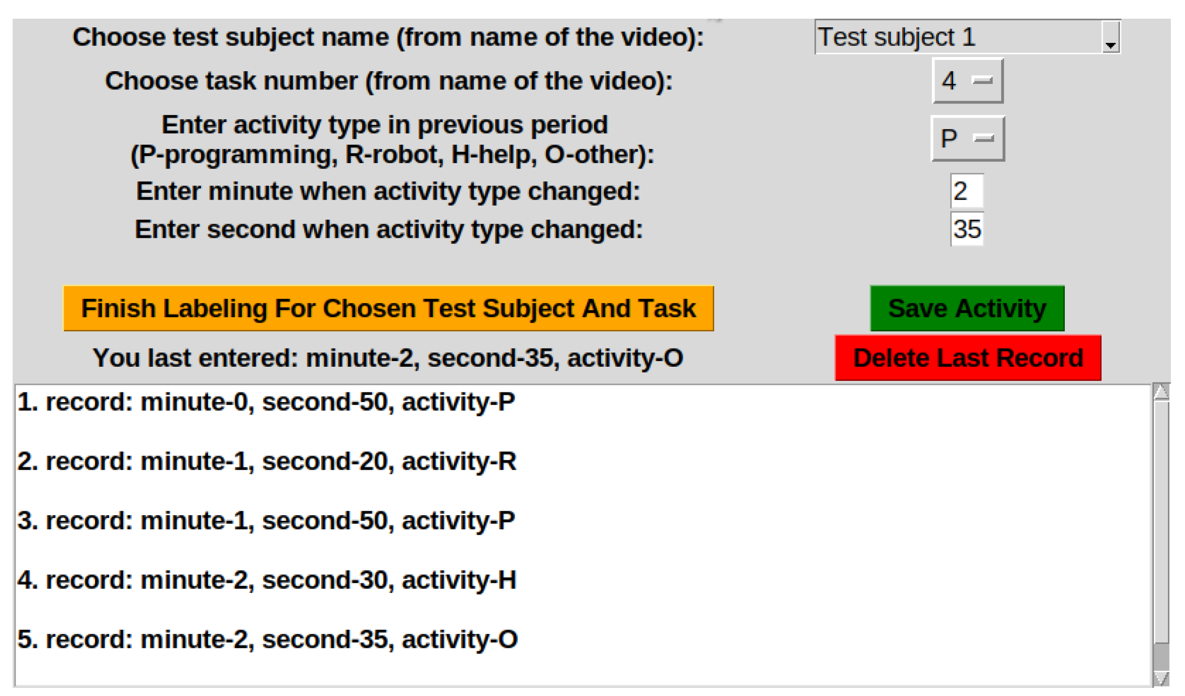
To label activities for experiment participants, a simple desktop application called Video Labeler was developed. With it, 14 annotators labeled videos of all 32 participants (almost 23 h of the video material). They were instructed to enter labels only on activity type change. The labeling task was pretty straightforward because the activity type change moment was always clearly visible and there was a minimal chance of disagreement between annotators due to the non-existent subjectivity component. Therefore, we used one annotator per video. A screenshot of Video Labeler is shown in Figure 1.

After obtaining the data about gender, tasks, and activity types for each participant, we needed to predict emotions on their faces. In each second of the video, the face was detected using SSD [31]. Since we wanted to eliminate face detection of extremely tilted faces when participants were looking far away from the camera, we discarded all detected faces if the model’s confidence level of the detection was under $95\%$. It is important to mention that it was possible that sometimes there were multiple faces in front of the camera. This would happen when a participant was asking for help. In these situations, we kept only the face with the largest detected bounding box area. Finally, in order to automatically label extracted faces with emotions, machine learning models were developed and used. Since most of the data sets and models were developed specifically for either lab-controlled or in-the-wild FER, and our use case is somewhere in between, we had to tailor both the FER models and data sets used for their training to our specific use case.

3.1. Emotion Recognition Models

To find the best models for FER in the active classroom environment where students are expected to constantly move their heads and not look directly into the camera, we investigated both traditional and deep learning algorithms in combination with categorical FER.

3.1.1. Data Set

In order to enable the predictive models to work properly in the active classroom environment, we combined both lab-controlled and in-the-wild standard emotion recognition data sets: CK+, FER-2013, and SFEW. These data sets were used to train our FER models. Used data set statistics are presented in

Table 2. Data set summary.

Class	Starting (3929 Total)			Final (3950 Total)
	CK+	FER-2013	SFEW	Train	Validation	Test
Anger	57	414	178	417	104	131
Happiness	84	417	198	453	114	142
Neutral	105	395	150	418	104	130
Other	126	374	164	426	106	133
Sadness	70	430	172	429	108	135
Surprise	87	412	96	385	96	119
Total	529	2442	958	2528	632	790

.

The CK+ data set has a set of images for each test subject and each of the following emotions: anger, disgust, fear, happiness, sadness, surprise, and contempt. For a specific emotion, images were recorded gradually from a neutral emotion to the targeted emotion that the subject was asked to show. Hence, we used only the first and the last image. The first image was gathered only once for each test subject from CK+ data set in order to avoid having class imbalance due to the large number of neutral class images. The contempt class was not used. From FER-2013, we hand-picked images for each class that were correctly labeled in our opinion. In our final data set, the most common examples are images from FER-2013 data set. This data set was labeled with the following emotions: anger, disgust, fear, happiness, sadness, surprise, and neutral. Finally, we added all the images from the SFEW train set which was labeled with same categorical emotion labels as FER-2013 data set.

To adjust the data set to the expected FER in the classroom for our experiment, class other was created by merging all images labeled as fear or disgust into one class, under the assumption that students will not show emotions of fear or disgust during programming and working with the robot. Furthermore, it is important to note that we discarded images with children’s faces due to the fact that all participants in our experiment were adults.

As a result, we had 3929 images in our starting data set. Some images from the data set were already cropped in advance to show only the face (mostly for the FER-2013 data set) while others required detection and extraction of the faces manually. Additionally, the SFEW data set had images with several faces in one image showing the same emotion. Therefore, we extracted them into separate images which increased the final data set face number to 3950. For face detection, we used the Single Shot MultiBox Detector (SSD) [31]. If the model had confidence higher than $50\%$, we assumed that the detected object was a face. Finally, images were resized to match the size of 300 × 300 pixels, converted to grayscale, and Contrast Limited Adaptive Histogram Equalization (CLAHE) was applied.

The data set splits into train, validation, and test sets were stratified to avoid the class imbalance problem. Furthermore, the splits were created with the same random state in advance to enable model comparison. We trained all the models on the same train set, tuned hyperparameters on the same validation set, and compared prediction success on the same unseen testing data.

3.1.2. Machine Learning Models

We implemented and tested traditional (e.g., Support Vector Machine (SVM)) and deep learning (e.g., CNN) methods in Python using specialized machine learning (ML) libraries scikit-learn (https://scikit-learn.org/stable/ (accessed on 28 February 2022)) and Pytorch (https://pytorch.org/ (accessed on 28 February 2022)). Experiments with deep learning models were performed on Google Colab (https://colab.research.google.com/ (accessed on 28 February 2022)).

The starting approach for solving the FER problem was to use facial landmarks for crafting the features which were inserted into the traditional machine learning model. Facial landmarks were located using the C++ library dlib [32] in combination with Python. The 68 facial landmarks form the starting points set $P={\left\{\left(x_i,y_i\right)\right\}}_{i=1}^{68}$.

Since humans can show the same emotion in different parts of the image due to head movement, face shape etc., we performed scaling of original facial landmarks to mitigate that effect:

$$\begin{array}{c}\hfill P_{scaled}={\left\{\left(\frac{x_i-\overline{x}}{max\left|P\right|},\frac{y_i-\overline{y}}{max\left|P\right|}\right)\right\}}_{i=1}^{68}\end{array}$$

where $(\overline{x},\overline{y})$ refers to the mean of the set P i.e., a centroid on the face. The denominator is the largest absolute value among x and y values from the set P. Moreover, we created additional features using distances from each facial landmark to the centroid of all facial landmarks. The distance features were calculated by applying L2-norm on the facial landmarks from the standardized set $P_{std}$ and its centroid $({\overline{P}}_{std,x},{\overline{P}}_{std,y})$:

$$\begin{array}{c}\hfill P_{dist}={\left\{\sqrt{{(P_{std,i,x}-{\overline{P}}_{std,x})}^2+{(P_{std,i,y}-{\overline{P}}_{std,y})}^2}\right\}}_{i=1}^{68}\end{array}$$

where the standardized set of facial landmarks was defined as:

$$\begin{array}{c}\hfill P_{std}={\left\{\left(\frac{x_i-\overline{x}}{\widehat{{\sigma }_x}},\frac{y_i-\overline{y}}{\widehat{{\sigma }_y}}\right)\right\}}_{i=1}^{68}\end{array}$$

with $\widehat{{\sigma }_x}$, $\widehat{{\sigma }_y}$ denoting estimated standard deviation of x and y points from the starting points set P, respectively.

Finally, features from $P_{scaled}$ and $P_{dist}$ were concatenated into the final feature vector with a total number of elements equal to 204. The final feature vector included both x and y values of the $P_{scaled}$ set and all distance values from the $P_{dist}$ set. Furthermore, to filter out redundant features, univariate feature selection was applied. Depending on the f-value from an Analysis of Variance (ANOVA) test, 120 final features were chosen that showed statistically significant differences across the 6 emotion classes.

Numerous traditional models were tried out on extracted features: SVM, Logistic Regression (LR), K-nearest Neighbors (KNNs), Random Forest Classifier (RF), and eXtreme Gradient Boosting Classifier (XGBoost). We opted for the SVM since it generalized best on the crafted features.

The SVM model was performing sufficiently well enough in the static case, but seemed to generalize badly when the experiment participant was not looking directly at the camera due to head rotation. This could certainly be explained by the inability of dlib’s facial landmarks predictor to properly position facial landmarks on a tilted face. Thus, we turned to the development of deep models using our own and pre-trained CNNs.

First, we developed our own CNN for FER (EM-CNN), whose architecture is shown in

Table 3. EM-CNN architecture.

Layer Type	Number of Filters (Channels)	Filter (Kernel) Size	Stride	Padding	Output Size
Input Layer	-	-	-	-	300 × 300 × 3
Convolutional Layer	16	11	1	1	295 × 295 × 16
Batch Normalization	-	-	-	-	295 × 295 × 16
ReLU	-	-	-	-	295 × 295 × 16
Max Pooling Layer	1	2	2	0	147 × 147 × 16
Convolutional Layer	32	7	1	1	144 × 144 × 32
Batch Normalization	-	-	-	-	144 × 144 × 32
ReLU	-	-	-	-	144 × 144 × 32
Max Pooling Layer	1	2	2	0	72 × 72 × 32
Convolutional Layer	64	6	1	1	70 × 70 × 64
Batch Normalization	-	-	-	-	70 × 70 × 64
ReLU	-	-	-	-	70 × 70 × 64
Max Pooling Layer	1	2	2	0	35 × 35 × 64
Convolutional Layer	128	5	1	1	35 × 35 × 128
Batch Normalization	-	-	-	-	35 × 35 × 128
ReLU	-	-	-	-	35 × 35 × 128
Max Pooling Layer	1	2	2	0	17 × 17 × 128
Convolutional Layer	256	3	1	1	17 × 17 × 256
Batch Normalization	-	-	-	-	17 × 17 × 256
ReLU	-	-	-	-	17 × 17 × 256
Max Pooling Layer	1	2	2	0	8 × 8 × 256
Fully Connected Layer	-	-	-	-	16,384

. Input to the EM-CNN was a resized grayscale image to match the 300 × 300 dimensions with 3 input channels. Since grayscale images have only one channel, the three channels were simulated by copying the first channel two times. We added image augmentation to the training set including random horizontal flip and random image rotation where the angle of the rotation was chosen randomly from the interval $[-45,45]$. Lastly, images from train, validation, and test sets were standardized using a mean of $0.516$ and a standard deviation of $0.247$. The mean and standard deviation values were calculated a priori on the whole data set. This network performed better than our SVM model, as is given in the next section.

However, the data set of almost 4000 images turned out to be too small to train the EM-CNN from scratch in order to obtain a significant generalization performance improvement over the SVM with handcrafted features.

Therefore, we fine-tuned two popular pre-trained CNNs: ResNet-34 [33] and Inception-v3 [34]. At the end of these networks, the final fully connected layer was appended to enable classification into 6 classes.

For the training phase, Inception-v3 uses two output layers. The primary output is a linear layer at the network’s end, while the second output is an auxiliary one. For the testing phase, only the primary output is used. Input image size for Inception-v3 is 299 × 299. Thus, the data set images were shrunk a little before being fed into the network’s input to match its requirements.

ResNet-34 is a deep residual convolutional neural network with 34 layers. It gave better results than ResNet-18 and ResNet-152 with 18 and 152 layers, respectively. Input image size for ResNet-34 is 224 × 224.

The following pre-processing steps were the same for Inception-v3 and ResNet-34. Both networks expect three channels at the input, so the grayscale images from the data set were duplicated onto the two remaining channels. Next, the same pre-processing pipeline was applied to the train set as for EM-CNN: random horizontal flip, random rotation, and standardization. Validation and test sets were only standardized.

3.1.3. Model Selection

We compare four models: SVM with handcrafted features, EM-CNN, fine-tuned Inception-v3, and fined-tuned ResNet-34. All models were trained, validated, and tested on the same splits of the original data set.

For our SVM model, a radial basis function kernel was used. We tuned regularization parameter C and kernel coefficient $\gamma$ using grid search with 5-fold cross validation. Both parameters for grid search took on values from the following set: $\{2^{-15},2^{-14},...,2^9,2^{10}\}$. The best hyperparameters were: $C=16$, $\gamma =0.25$.

CNNs had different hyperparameters to optimize with respect to SVM, but the same with respect to each other. The best obtained hyperparameters for the three CNNs are presented in

Table 4. Hyperparameters which gave best results on the validation set for CNNs: EM-CNN, fine-tuned Inception-v3 (Inception), fine-tuned ResNet-34 (ResNet). FC stands for fully connected. All CNNs used Adam as optimizer and utilized the early stopping method.

CNN	Architecture	Best Learning Rate	Learning Rate Scheduler
EM-CNN	See Table 3	0.0005	Multiplicative (factor = 0.99)
Inception	Same as [34] with FC layer on top	0.0005	Multiplicative (factor = 0.95)
ResNet	Same as [33] with FC layer on top	0.0006	Multiplicative (factor = 0.99)

. We explored Stochastic Gradient Descent (SGD) and Adam as optimizers. Adam gave better results. The optimal architecture for EM-CNN is given in Table 3. Pre-trained CNNs were examined as fixed feature extractors and as fine-tuned models. Both Inception-v3 and ResNet-34 worked better when fine-tuned. For training our deep models, we tried learning rates of different orders of magnitude. The best performance was obtained when the learning rate was of the order of magnitude of ${10}^{-4}$. In addition, we tried training with and without the learning rate scheduler. The better performance on the validation set was achieved when we used the learning rate scheduler in contrast to keeping the learning rate fixed during the training phase. For all models, the best learning rate scheduler was the multiplicative one. This scheduler multiplies the learning rate of each parameter group with the multiplicative factor in each epoch. Hyperparameters for CNNs were optimized using randomized search. Lastly, early stopping was implemented that tracked changes in accuracy on the validation set. If there was no improvement on the validation set in 50 consecutive epochs, the training phase was stopped. For each CNN, the parameters that were chosen as optimal were ones that achieved the highest score on the validation set independent of the early stopping method.

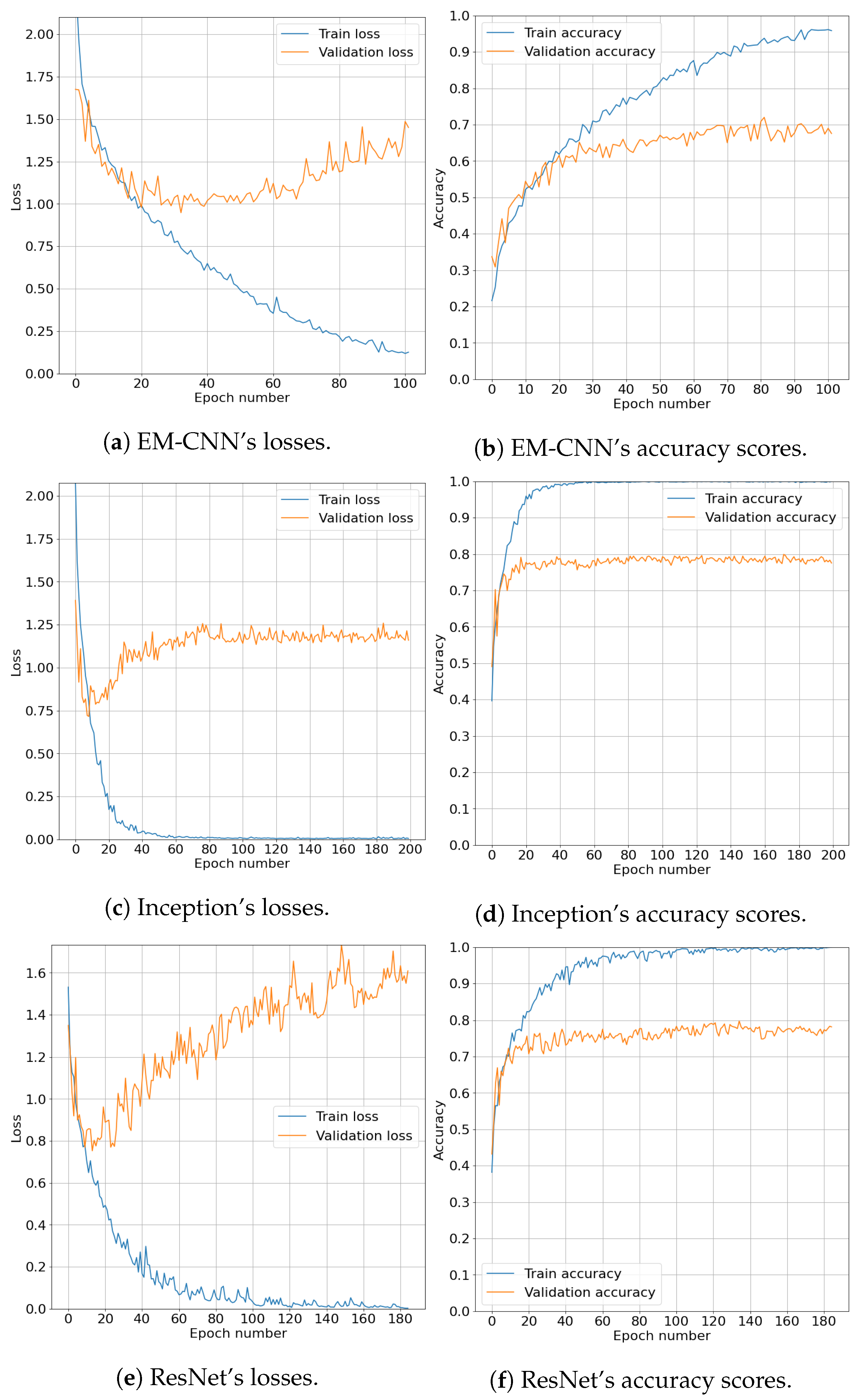
Plots of cross-entropy losses and accuracy scores over epochs are given in Figure 2. A maximum number of epochs was not set in advance since the early stopping method was used. Hence, every CNN has a different final number of epochs on the x-axis. Generally speaking, all CNNs followed similar trends. Loss on the train set dropped almost monotonically, while loss on the validation set dropped until some point where it started to grow again. Accuracy scores on the train set gravitated towards $1.0$, while the validation set scores rose to a score between $0.6$ and $0.8$ and oscillated around that value until the early stopping was activated and stopped the training phase.

Table 5. Precision (P), recall (R), F1-score (F1), and accuracy (Acc) on the test set for all used models given in percentages: SVM, EM-CNN, fine-tuned Inception-v3 (Inception), and fine-tuned ResNet-34 (ResNet). Best scores for every metric are denoted in bold.

Model	Metric
	P	R	F1	Acc
SVM	58.617	59.328	57.978	59.367
EM-CNN	65.958	65.77	65.622	65.57
Inception	79.033	78.994	78.811	78.987
ResNet	77.002	76.417	76.259	76.456

contains evaluation results on the test set for the four previously described models. The following standard evaluation metrics were chosen: macro precision, macro recall, macro F1-score, and accuracy. Fine-tuned Inception-v3 proved to have the highest score on the test set for every evaluation metric. ResNet-34 followed with a slight difference. EM-CNN and SVM had greater drops in all evaluation metrics. Given the results, each of the models learned fairly well to classify emotions into one of the six classes when we consider that the random guessing probability for classification into one of six classes equals $16.67\%$.

Two-tailed permutation tests were conducted on model pairs and the results are displayed in

Table 6. P-values of two-tailed permutation tests on model pairs: SVM, EM-CNN, fine-tuned Inception-v3 (Inception), and fine-tuned ResNet-34 (ResNet).

	SVM	EM-CNN	Inception	ResNet
SVM	-	$\mathbf{0.0003}$	<${\mathbf{10}}^{-\mathbf{5}}$	<${\mathbf{10}}^{-\mathbf{5}}$
EM-CNN	-	-	<${\mathbf{10}}^{-\mathbf{5}}$	<${\mathbf{10}}^{-\mathbf{5}}$
Inception	-	-	-	0.0542
ResNet	-	-	-	-

. The tests were performed only on macro F1-score since it is the most unbiased one of all the chosen metrics. P-values show how all the test results are statistically significant when using the Bonferroni corrected significance level of ${\alpha }_b=0.00167$ (starting significance level was $\alpha =0.01$), except the one between Inception and ResNet. Thus, we cannot claim that there is statistically significant difference in generalization performance between the two models. However, we can claim that SVM performed worst, followed by EM-CNN, while fine-tuned Inception-v3 and ResNet-34 performed best. Therefore, we decided to combine both fine-tuned CNNs for prediction on the videos from our FER classroom experiment.

4. Results

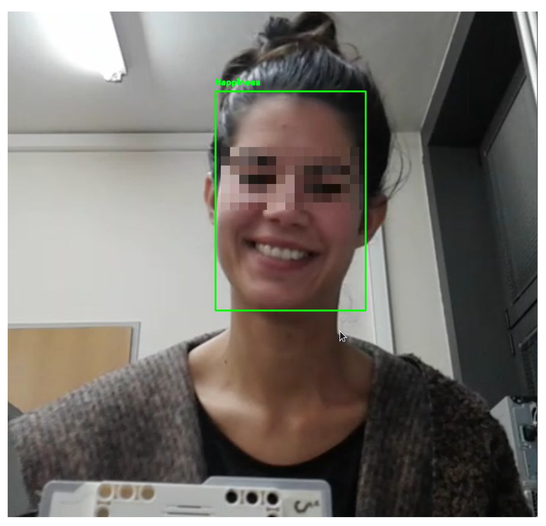
Based on the predicted emotions, labeled activities, stated gender, and extracted tasks, in this section we use statistical analysis methods to answer our research questions. Predictions of emotions in time were obtained by applying the developed models on the collected images of faces extracted from videos of experiment tasks. To obtain more robust predictions, we used prediction from both fine-tuned Inception-v3 and ResNet-34. An emotion was considered valid only if the prediction from both models applied to the extracted face was the same. In this way, we obtained 39,144 predicted emotions from roughly 23 h of video footage. This means that $48\%$ of all the footage was labeled with emotions. This is one of the reasons why there are parts in videos with no recorded emotion predictions. Additionally, the SSD did not detect the face in the image. However, this was not a problem since it does not matter at what exact second an emotion occurred, but it is important in what context the emotion appeared with respect to the task being solved, gender of the participant, and the activity type that was being performed when the emotion emerged. An example of the emotion prediction on the frame from one specific video, during the robot activity, is shown in Figure 3.

The total counts of predicted emotions in all videos for men and women separately and together are presented in

Table 7. Counts of predicted emotions from videos for male and female participants in the classroom experiment. Frequencies are sorted in descending order by the total number of the predicted emotions (fourth column).

Emotion	Men	Women	Both
Neutral	9634	7185	16,819
Sadness	8080	8090	16,170
Happiness	1106	1902	3008
Anger	410	966	1376
Other	282	776	1058
Surprise	321	392	713

. The process of obtaining predictions from 23 h of video footage took 4 h and 30 min on an Intel^® Core™ i7-6700HQ processor and a computer with 8 gigabytes of RAM. Therefore, for one second of the video, face detection and prediction, with the help of the two chosen models, are obtained within $0.2$ s. We can observe that the most common predicted emotions were neutral and sadness regardless of gender. Such high numbers for a neutral emotion were expected because for the most of the experiment participants were programming and showed no emotions. On the other hand, high numbers for the emotion of sadness were an unexpected outcome. Fortunately, there is a simple explanation. Since the cameras were set up to record faces slightly from below, neutral faces viewed from below can appear sad. Since the neutral emotion (and in our case sadness) was the default facial expression in our experiment, for the remainder of the analysis we used only happiness, anger, and surprise. The emotion other was not used since it represents all other unspecific emotions, and therefore is hard to interpret.

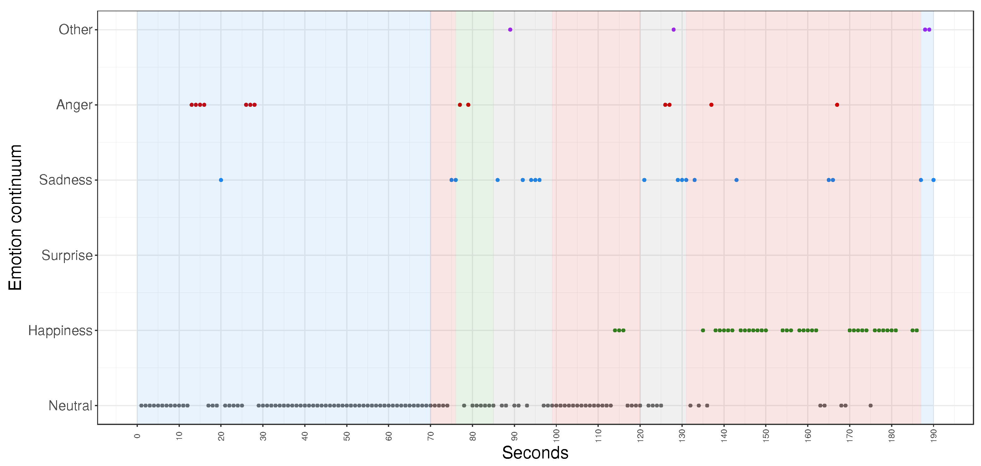
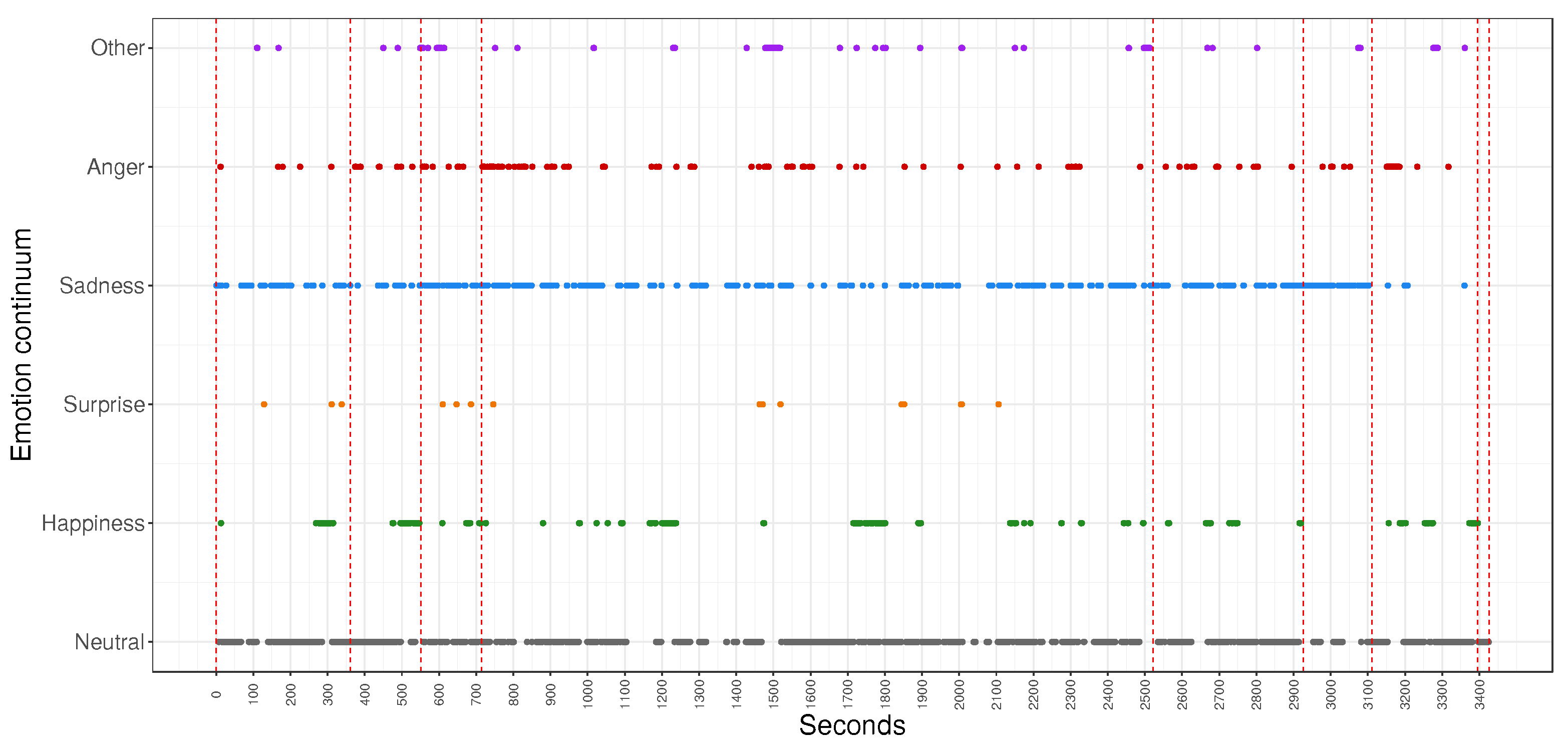
It is interesting to observe the timeline of predicted emotions for just one particular participant and one task from the experiment (Figure 4). The y-axis shows a so-called continuum of emotions where emotions are presented gradually (1: neutral, 2: happiness, 3: surprise, 4: sadness, 5: anger, 6: other). This particular example contains occurrences of all considered emotions except surprise with respect to all types of activities whose duration is shown using a shaded background. We can infer that the most frequently shown emotion was neutral and that this specific participant spent most of the time at the beginning of the task doing programming (blue shaded background) while at the end of the task the participant spent most of the time using the robot (red shaded background). It can also be noticed that here the emotion of anger occurred most often during programming while the emotion of happiness emerged mostly during the experimentation with the robot, while the class other appeared the least (when we do not consider the absence of the emotion of surprise).

Figure 5 shows predicted emotions in time for all eight tasks of the same participant as in Figure 4. Emotions neutral and sadness come to the fore and both can be interpreted as neutral as was already discussed. Since not all participants in the experiment spent the same or even a similar amount of time solving the same or distinct tasks, we turned to analysis of emotions with respect to activity types, gender, and tasks through probability distributions and statistical tests without the consideration of the absolute time component.

For the statistical analysis of the connection between emotions, activities, and gender, the probability distributions were employed whose parameters were estimated using the maximum likelihood estimation. The probabilities were estimated with the equation:

$$P({\mathit{variable}}_1=v_1|{\mathit{variable}}_2=v_2\wedge {\mathit{variable}}_3=v_3)=\frac{C({\mathit{v}}_1,{\mathit{v}}_2,{\mathit{v}}_3)}{C({\mathit{v}}_2,{\mathit{v}}_3)}$$

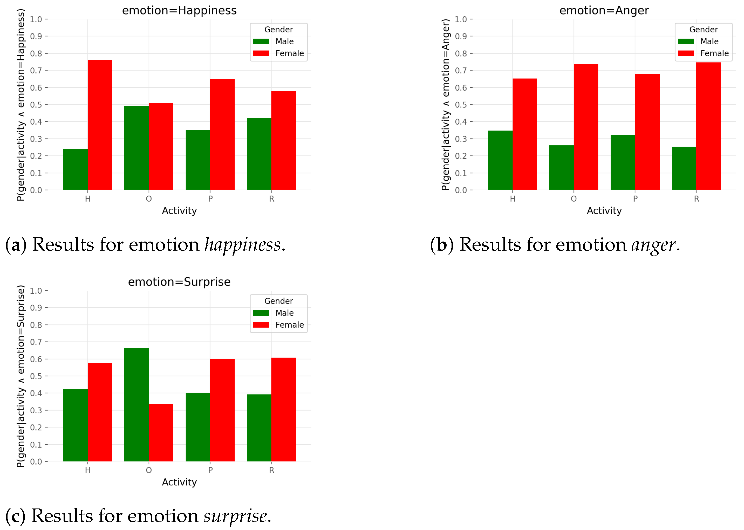
where C denotes frequency. Each of the variables ${\mathit{variable}}_1,{\mathit{variable}}_2,{\mathit{variable}}_3$ can describe either emotion, activity, or gender. ${\mathit{v}}_1,{\mathit{v}}_2,{\mathit{v}}_3$ correspond to concrete values of these three variables. Specifically, for probability distributions from Figure 6, the following assignment is valid: ${\mathit{variable}}_1=gender,{\mathit{variable}}_2=activity,{\mathit{variable}}_3=emotion$. Probabilities sum to $1.0$ inside variable gender which leads to the fact that bar plots are comparable only inside that variable. Each graph shows one of the three chosen emotions: happiness, anger, and surprise. Figure 6 shows that for the most of the activities, female participants showed emotions of happiness, anger, and surprise with higher probability than male participants. The outlier is the emotion of surprise and activity other from Figure 6c where the trend is reversed. Additionally, female and male participants showed with similar probability the emotion of happiness during the activity other. Further, the female participants expressed with very high probability the emotion of happiness during the activity help and had very high probability of showing the emotion of anger during the activity robot.

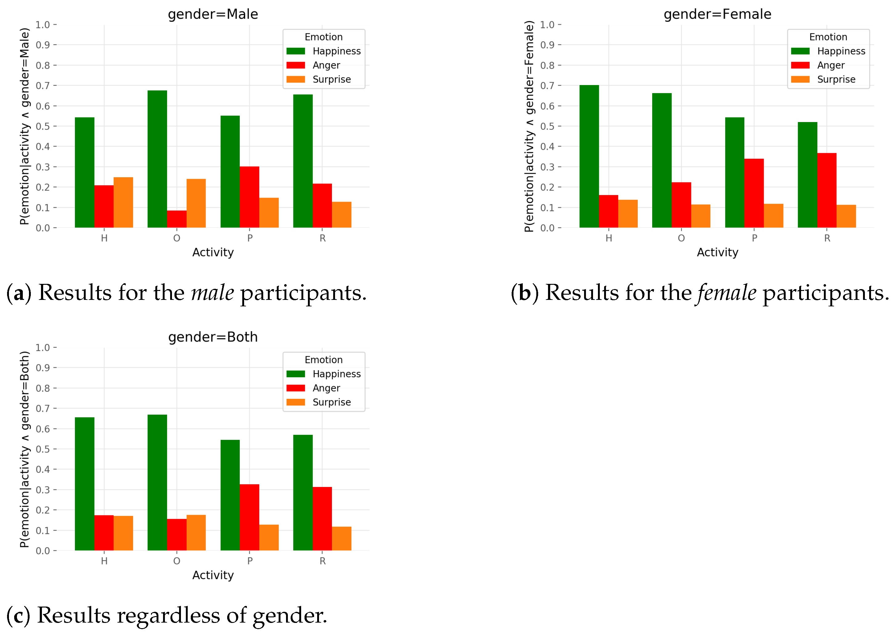
Similarly to the previous analysis, the MLE method was used to estimate the probability distributions $P\left(\mathit{emotion}\right|\mathit{activity}\wedge \mathit{gender})$. Consequently, the following assignment is valid: ${\mathit{variable}}_1=emotion,{\mathit{variable}}_2=activity,{\mathit{variable}}_3=gender$. Probabilities sum to $1.0$ inside the variable emotion. The results are shown in Figure 7. The conclusion that can be drawn is that regardless of gender, the emotion of happiness was shown with the highest probability (in this simplified scenario where only emotions of happiness, anger, and surprise were considered) within all types of activities. Anger was the second most probable emotion to appear and the emotion of surprise had the lowest probability. Only during the help and other activities did male participants show more surprise than anger. As a result, surprise and anger appeared equally regardless of gender in those two activities.

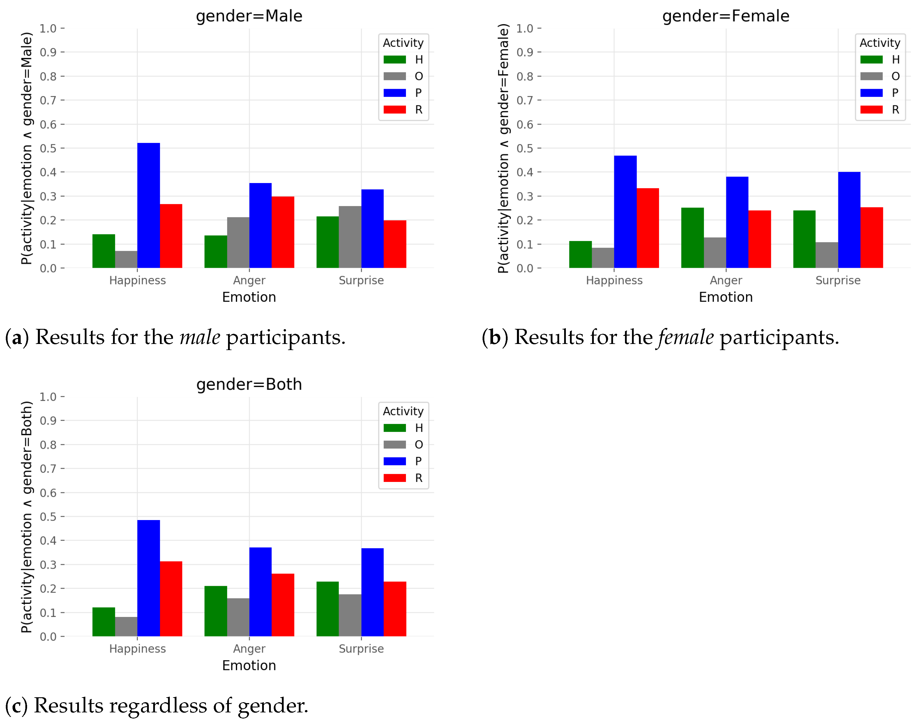
The last analysis using probability distributions describes estimated probabilities $P\left(\mathit{activity}\right|\mathit{emotion}\wedge \mathit{gender})$ with MLE. Variables were assigned as follows: ${\mathit{variable}}_1=activity,{\mathit{variable}}_2=emotion,{\mathit{variable}}_3=gender$. Probabilities sum to $1.0$ inside variable activity. This type of visualization enables the observation of the probability of individual emotions appearing in the relationship with activity types. It is quite interesting to notice how the shapes of distributions for female experiment participants from Figure 8b dictated shapes of distributions regardless of gender from Figure 8c. The inference is being imposed that, regardless of gender, the probability that some of the emotions of happiness, anger, or surprise will appear is highest during the activity programming. Right after programming, the most probable time for emotions to appear is during the activity robot if we observe the state shown in Figure 8c, although the appearance of the emotion surprise in the activities help and robot seems equally probable.

In order to analyze the dependency between emotions and activities through tasks, ${\chi }^2$ tests of independence were carried out. The results are given in

Table 8. P-values of ${\chi }^2$ tests of independence between the categorical variables emotion and activity. The statistical tests were conducted depending on gender and tasks. Symbol $\perp \perp$ indicates the existence of dependency between the two variables. Bold p-values denote proved dependency between emotions and activity types when considering the chosen significance level of $\alpha =0.01$.

Task	H0: emotion activity H1: emotion$\perp \perp$activity
	Men	Women	Both
1	<$\mathbf{0.001}$	$\mathbf{0.001}$	<$\mathbf{0.001}$
2	0.348	<$\mathbf{0.001}$	<$\mathbf{0.001}$
3	<$\mathbf{0.001}$	0.199	<$\mathbf{0.001}$
4	<$\mathbf{0.001}$	<$\mathbf{0.001}$	$\mathbf{0.002}$
5	0.447	<$\mathbf{0.001}$	<$\mathbf{0.001}$
6	0.047	0.022	0.043
7	<$\mathbf{0.001}$	<$\mathbf{0.001}$	<$\mathbf{0.001}$
8	<$\mathbf{0.001}$	<$\mathbf{0.001}$	<$\mathbf{0.001}$
All tasks	<$\mathbf{0.001}$	<$\mathbf{0.001}$	<$\mathbf{0.001}$

. With chosen significance level of $\alpha =0.01$, we proved that there exists dependency between the three analyzed emotions and four types of activities for almost every task. For men, the dependency was not proved for tasks 2, 5, and 6 while, for women, for tasks 3 and 6. If we look at Table 1, it is interesting to observe that tasks 2 and 5 were short and just checked understanding of the previous tasks. They were the same as task 1 with respect to the used command, but required change in the parameters. Task 3 also did not introduce new commands but required use of mathematics or a trial and error approach. In task 6, participants needed to copy a prepared program in advance and discover the effect of the program on the robot’s behavior. Since the approach to these tasks was different from the others, that could explain why the test results were not significant. However, if we consider all tasks together, regardless of the gender of the experiment participants, there exists dependency between showing the emotion of happiness, anger, or surprise and the activity type that was being performed by the participant at the moment of showing the emotion. ${\chi }^2$ tests showed that there exists dependency between emotions and activities for the classroom experiment on the whole.

5. Discussion

During the experiment and analysis of the results, we noticed some potential validity threats to our research. The first big threat is that experiment participants might have changed their emotional behavior due to the fact that they knew they were being recorded with a camera while participating in the experiment. This is known as the Hawthorne effect [35] which could have been avoided by not telling the participants that they were going to be recorded, and asking them after the experiment if they wished for us to delete the recorded footage of them. However, this could have resulted in many of them asking us not to use their data for our research, so asking the participants to comply with our requirements before the experiment started seemed the best solution. The second big threat is potentially the selection bias since our experiment participants were mostly master’s and PhD students. Nonetheless, this only limits the selection in the aspect of the age range. Participants were still randomized in the sense that they came from different study disciplines. Regarding the conduction of the classroom experiment, we note that the tablet camera was not positioned in the optimal way and the faces were recorded tilted downward, resulting in a lot of sadness predictions instead of neutral. However, since the tablet cameras were the only available recording equipment, we positioned them in the best possible way we could. Furthermore, by applying stricter conditions on the behavior of the participants in the experiment, we could have limited the appearance of the activity type other. Nonetheless, we believe that this would have only accentuated the Hawthorne effect. Finally, although the annotation of the video data of the experiment with activity types was a pretty straightforward task and we opted to use one annotator per video, it would always be better to use two or more annotators per video to avoid potential labeling errors.

In the future work, we would like to collect more data for learning of the models, and re-conduct the classroom experiment with better camera positioning and stricter conditions on the behavior of the participants in the experiment. Additionally, we would like to explore if using the available audio data from the video recordings would enhance the quality of emotion predictions.

6. Conclusions

The goal of this study was to investigate the dependency of shown emotion, the activities, tasks, and gender during a robotics workshop, which is an example of an active teaching setting in the classroom. The tasks were given sequentially, from easier to harder, by introducing new commands and concepts. The experiment participants stated their gender, while the activities (programming, robot, help, other) were manually labeled by annotators. The most demanding part was to detect emotions. Therefore, much of the work was done to develop appropriate emotion recognition models. The training data for these models were collected from images of three well-known data sets for emotion recognition: CK+, FER-2013, and SFEW. Four models were developed on the collected data: one with the help of traditional machine learning and three using deep learning methods. The models were thoroughly compared by measuring prediction success on the test set and two of the models were selected to predict emotions on videos of the robotics workshop. The best models were fine-tuned Inception-v3 and ResNet-34. Their application enabled us to carry out the statistical data analysis, which provided insights into the relationship between emotions, gender, tasks, and types of activities and at the same time revealed answers to our research questions. Experiment participants mostly showed a neutral emotion during the classroom experiment. The most common emotions (neutral and sadness) were eliminated from the analysis and only emotions of happiness, anger, and surprise were statistically investigated. Female participants showed emotions of happiness, anger, and surprise more frequently and more noticeably (e.g., anger during the robot activity and happiness during the help activity) than male participants. Within all types of activities, the emotion of happiness was the most likely to appear. Participants were the most likely to show emotions of happiness, anger, or surprise during the activity programming. Statistical tests showed that there is dependency between showing the three chosen emotions and the four activities during the classroom experiment. The stated conclusions prove that FER can be used to evaluate the effect of active teaching methods in the physical classroom.