Article

Reinforcement-Learning-Based Decision and Control for Autonomous Vehicle at Two-Way Single-Lane Unsignalized Intersection

1
State Key Laboratory of Automotive Simulation and Control, Jilin University, Changchun 130025, China
2
College of Mechanical and Vehicle Engineering, Chongqing University, Chongqing 400044, China
3
Changan Automobile Intelligent Research Institute, Chongqing 710199, China
4
Department of Aeronautical and Automotive Engineering, Loughborough University, Leicestershire LE11 3TU, UK
5
Faculty of Transportation Engineering, Kunming University of Science and Technology, Kunming 650500, China
*
Authors to whom correspondence should be addressed.
Electronics 2022, 11(8), 1203; https://doi.org/10.3390/electronics11081203
Submission received: 8 March 2022 / Revised: 4 April 2022 / Accepted: 8 April 2022 / Published: 10 April 2022

Abstract

:
Intersections have attracted wide attention owing to their complexity and high rate of traffic accidents. In the process of developing L3-and-above autonomous-driving techniques, it is necessary to solve problems in autonomous driving decisions and control at intersections. In this article, a decision-and-control method based on reinforcement learning and speed prediction is proposed to manage the conjunction of straight and turning vehicles at two-way single-lane unsignalized intersections. The key position of collision avoidance in the process of confluence is determined by establishing a road-geometry model, and on this basis, the expected speed of the straight vehicle that ensures passing safety is calculated. Then, a reinforcement-learning algorithm is employed to solve the decision-control problem of the straight vehicle, and the expected speed is optimized to direct the agent to learn and converge to the planned decision. Simulations were conducted to verify the performance of the proposed method, and the results show that the proposed method can generate proper decisions for the straight vehicle to pass the intersection while guaranteeing preferable safety and traffic efficiency.

1. Introduction

With the rapid development of automatic-driving technology, many functions of low-level advanced driver-assistance systems have been implemented in an increasing number of vehicles. However, for high-level automatic-driving systems, it is imperative to develop safer and more intelligent decisions and control for automated vehicles under increasingly complex traffic scenes. As a typical traffic scene with a high incidence of accidents, unsignalized intersections have been investigated by many researchers for decision making and control to promote driving safety and efficiency [1,2].
As a classical method, behavior prediction for surrounding vehicles in traffic environment has proved to be an efficient way of dealing with decision-making problems. Zyner et al. [3] leveraged the long short-term memory (LSTM) recurrent neural network (RNN) to predict the intention of the driver when a vehicle enters an intersection, contributing to the decision making of an autonomous vehicle. A decision-making framework is proposed by Samyeul in [4] for autonomous vehicles to predict the future trajectory of observed vehicles and to delineate the potentially dangerous collision area to help navigate the intersection safely and efficiently. In [5], a motion-planning method for autonomous vehicles is introduced via rapidly exploring the random-tree algorithm. To solve motion-planning problems in environments with dynamic obstacles, the algorithm combines the RRT algorithm and the configuration-time space to improve the quality of the planned trajectory. Ramyar et al. [6] present a data-driven technology using the Takagi–Sugeno fuzzy model to simulate and predict driver behavior at intersections, thereby further improving prediction accuracy.
Model predictive control (MPC) as a commonly used control method has been widely exploited in decision control of autonomous driving at intersections. In [7], a bilevel MPC algorithm is established for the coordination of autonomous vehicles at intersections, and a distributed sequential quadratic-programming (QP) method is leveraged to solve the intersection-level optimization problem. Zhao et al. [8] developed a collaborative-driving algorithm for connected and automated vehicles at unsignalized intersections based on MPC, and a decentralized controller was advanced to control each vehicle to pass through the intersection smoothly. A probabilistic model was devised to predict the trajectory of the target vehicle [9], and afterwards was integrated within a collision-avoidance model. Katriniok et al. proposed a distributed MPC approach that enables multiple vehicles to pass through an intersection simultaneously with a safe and efficient manner [10]. A study was conducted concerning the decision-making control in intersections with multiple surrounding vehicles [11], wherein a robust MPC is responsible for searching security breakthrough in the studied scene, and meanwhile, planning the optimal trajectory.
In recent years, partial observable Markov decision processes (POMDP) have been progressively employed for autonomous-driving decisions at intersections. Bouton et al. [12] defined the traffic problem at unsignalized intersections as a POMDP, and the Monte Carlo sampling method was adopted to solve the problem. Shu et al. [13] proposed a method for decision-making control for left-turning intelligent vehicles based on the key turning points at intersections, and a partially observable Markov model was employed to solve the optimal speed sequence in the left-turn process. Kye et al. [14] introduced an intent-aware autonomous-driving decision-making method at unsignalized intersections, where the intents of traffic participants were modeled as dynamic Bayesian networks, and the intent-aware decision-making problem was modeled as a POMDP based on the inference results. Hubmann et al. [15] considered the occlusion generated by static objects and dynamic objects at the same time, and a general autonomous-driving strategy based on POMDP was advanced under urban conditions. In [16], a POMDP framework was proposed for online autonomous driving in different situations.
Machine-learning algorithms, such as reinforcement learning (RL), are also widely exploited in the field of decision control. Deep RL (DRL) combines the perception ability of deep learning and the decision-making capability of RL, performing well in solving continuous motion-control problems [17,18]. Islee et al. [19] investigated the effectiveness of DRL in dealing with intersection decision-control problems. Through comparison study, a deep Q network enables the learning of strategies better than common heuristic methods for different indicators, such as traffic time and traffic rate; however, the generalization ability is limited. Shi et al. proposed a coordinated control method with proximal policy optimization in a vehicle-road-cloud integration system, and a policy of the connected vehicles was learned by RL to across the intersection safely [20]. Chen et al. [21] proposed an autonomous intersection-management system based on DRL, and a braking safety-control model was applied to ensure the safety of each autonomous vehicle at the intersection. Zhou et al. [22] established a vehicle-following model for intelligent vehicles based on RL to improve driving behavior at intersections. By specifying an effective reward function, the model can be learned and works well under different conditions to improve fuel consumption, safety, and driving efficiency.
In view of the research status of autonomous-driving decision making and control at integrated intersections, planning methods based on state-prediction results of environmental vehicles usually quantify the degree of risk of intersection collisions, and rule-based strategies are proposed to make decisions for intelligent vehicles. However, rule-based strategies exhibit poor generality, and the formulation of rules depends on the practical experience, greatly affecting the effectiveness of the algorithm. Problems in the decision and control of intelligent vehicles at intersections are complex and involve multifactor coupling [23]. Crossing an intersection is a complex driving behavior [24]; thus, it is necessary to simplify the intersection-scene model to a certain extent to make decision rules depending on the quantified degree of risk, leading to certain differences between the simplified scene and the actual scene [25]. Generally, a POMDP model requires a large amount of computation. Although Monte Carlo sampling can mitigate this concern, the required discretization of the motion space will also lead to deteriorated accuracy to some extent [13]. The method based on model prediction strongly relies on the accuracy of the established model; thus, many factors should be considered comprehensively in the modeling process to achieve a satisfactory control effect [8]. In contrast to the above methods, a specific control model is not required in RL due to its model-free characteristic. Decision making for straight intelligent vehicles at intersections is a continuous action-control problem, and thus it is well-believed that the decision-making control problem of intelligent vehicles at intersections can be solved by an RL method.
Motivated by these conditions, in this study, a decision-and-control model based on RL is designed. The main contributions of this study are as follows. (1) A method is proposed to judge the priority of crossing the intersection based on a speed prediction by an autoregressive integrated moving average (ARIMA), and to calculate the expected speed of an autonomous vehicle. (2) A decision-and-control model is constructed based on speed prediction and RL. The model incorporates the expected speed guided by the RL model to converge in the optimal direction, thereby saving the learning time of the agent. (3) A multiobjective decision-making control-effect-evaluation system is established with the consideration of success rate, speed punishment, safety, traffic efficiency, and comfort.
The remainder of this article is structured as follows. In Section 2, the geometric model of the road and the circular model of the vehicle body are established, and a mathematical analysis of the intersection confluence trajectory data is presented. In Section 3, a decision-and-control method based on speed prediction, RL, and evaluation methods is introduced in detail. In Section 4, the simulation and effects validation are addressed. Section 5 draws the main conclusions of this study.

2. Intersection Confluence Condition Modeling

To better analyze the decision-making process and explain the mathematical model of the subsequent decision-making control, the road-geometry model of the research object should be constructed first. When passing through the intersection, a vehicle generally has three directions to go, as shown in Figure 1a, where a-f represents the possible driving direction of the vehicle. As shown in Figure 1b, the relationship between two vehicles can basically be divided into three types: irrelevant (1–4), cross (5–7), and confluent (8,9). The areas with probability of collision are marked with a yellow box in the figures. Under the confluence condition, two vehicles will eventually drive into the same lane; therefore, the potential collision area is longer than in other conditions. This scene not only includes the decision-making and control problem in the process of two vehicles when passing through the intersection, but also contains the continuous influence between two vehicles after confluence. Therefore, this paper selects b and d for subsequent modeling and analysis.
Figure 2 illustrates the road-geometry model under the conditions of two-way single-lane confluence. Straight and turning vehicles enter the intersection from different junctions and eventually converge into the same lane. The center lines of the east–west and north–south lanes at the intersection are labeled as L C 1 and L C 2 , respectively; L S 1 through L S 4 represent the stop line at the intersection; and ( x , y ) is the confluence point of the two vehicles.

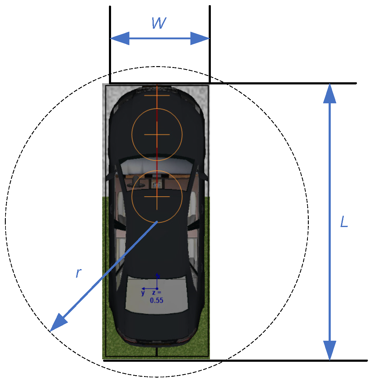
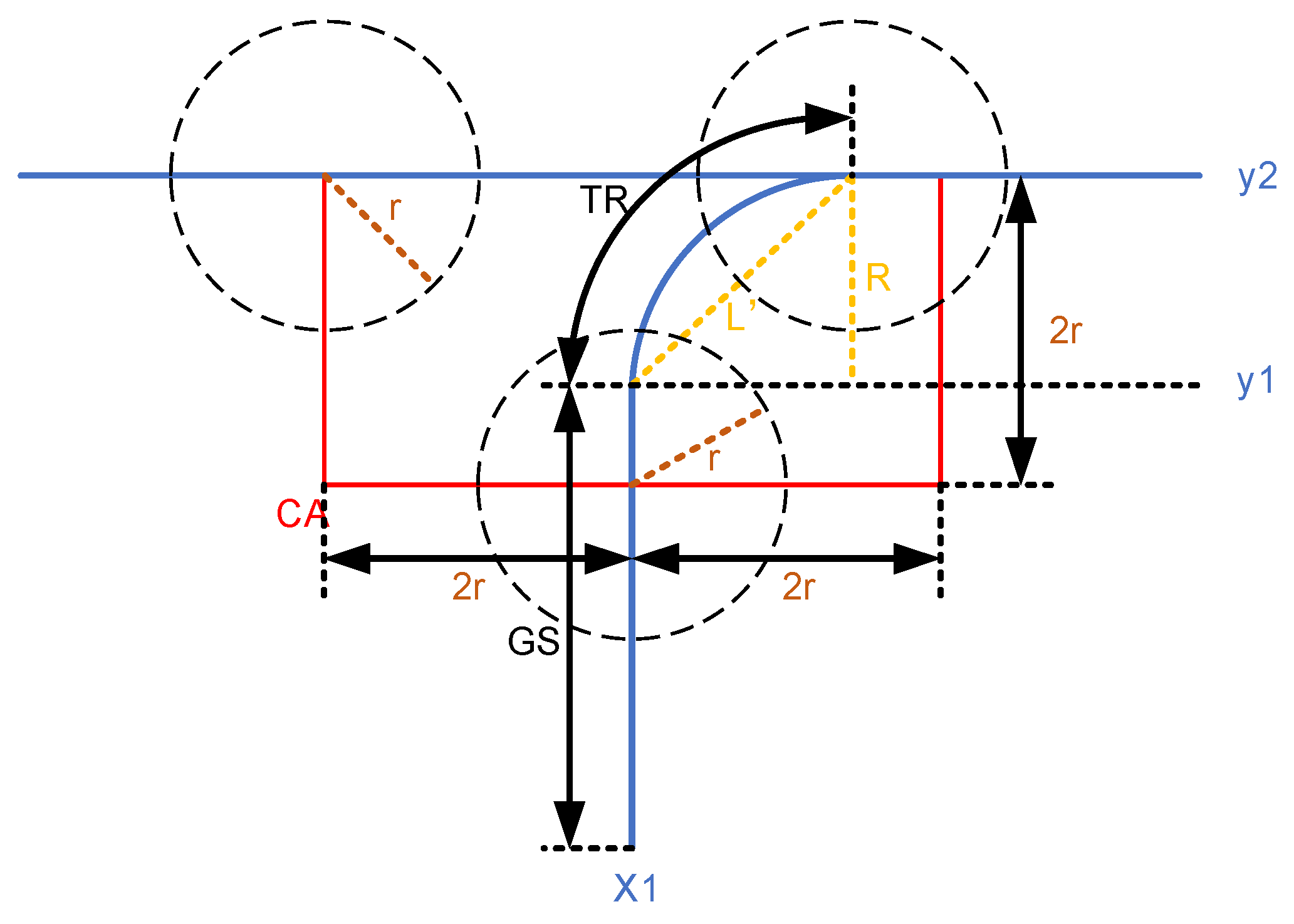
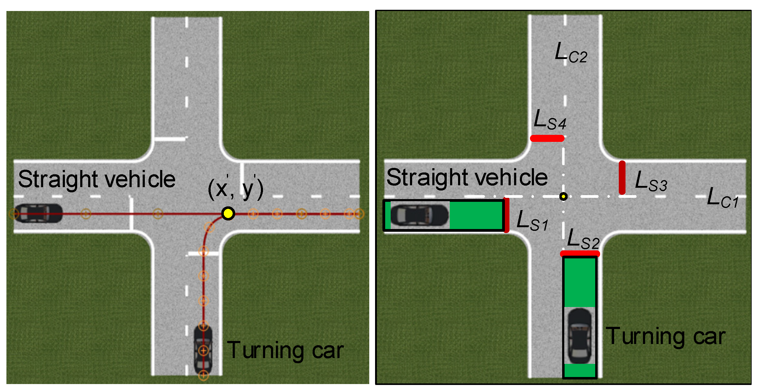
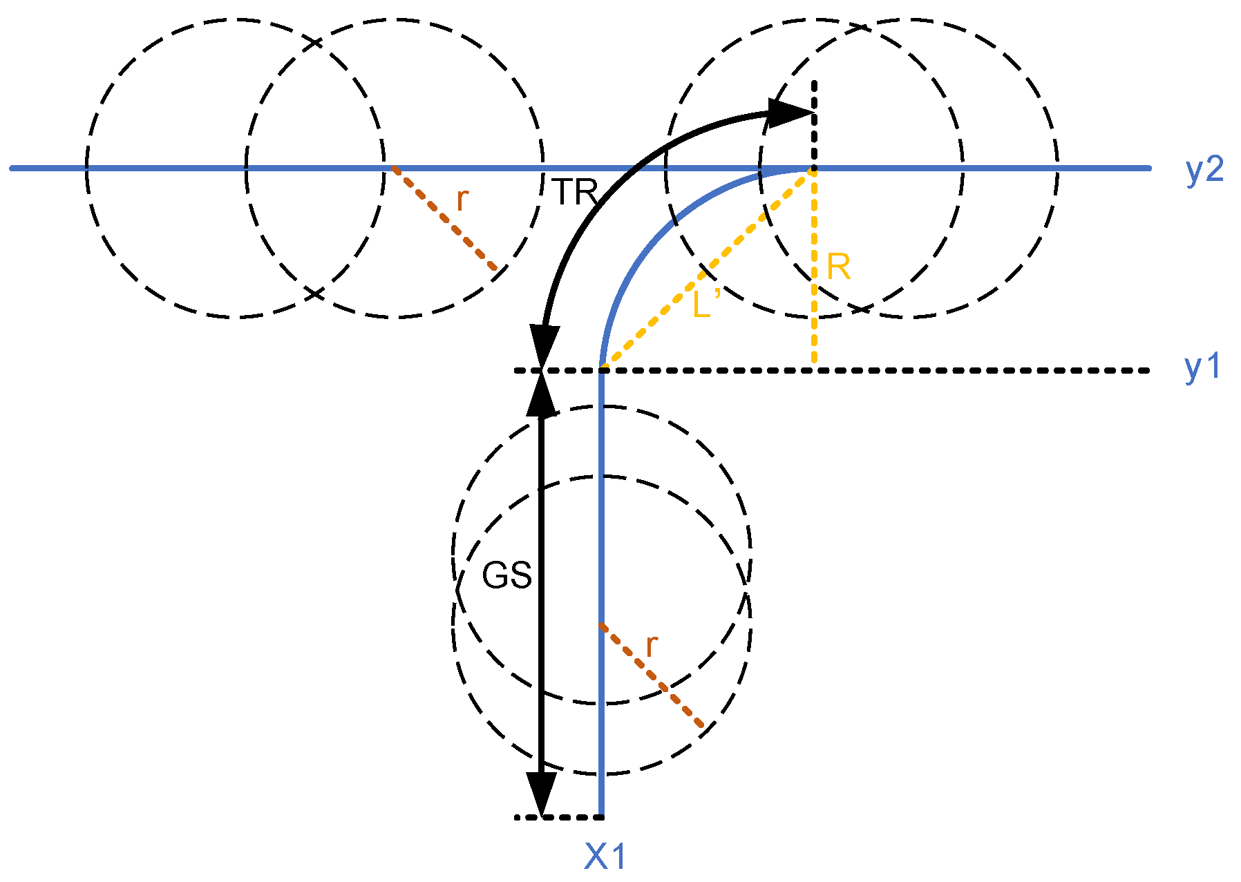
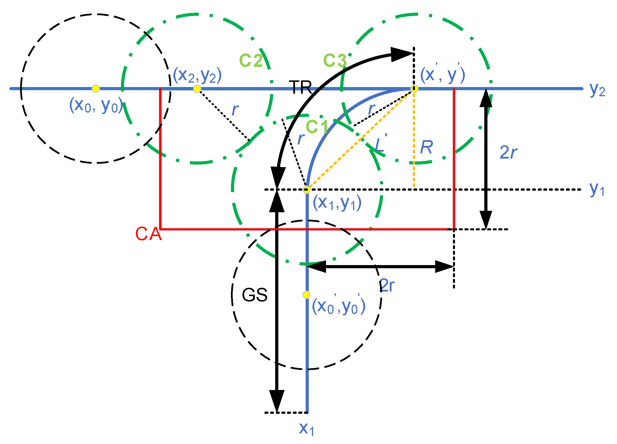
2.1. Circular Model of Vehicle Body

The trajectory shown in Figure 2 shows only the centroid movement process of the straight and turning vehicles without considering the actual geometric size of the vehicle. In a real driving scenario, the geometric size of the vehicle body cannot be ignored to avoid the potential risk of collision in the process of two vehicles converging at the intersection. Therefore, a circular model, which has been widely adopted in studies on vehicle collisions, is used to represent the vehicle body profile hereinafter, as shown in Figure 3. By this manner, the radius of the circular model can be calculated by
r = W 2 + L 2 2
where W and L denote the width and length of the vehicle, respectively; and r denotes the radius of the body circle.
Considering the circular model of the vehicle body, the actual motion trajectory of straight and turning vehicles under the confluence condition at the intersection is shown in Figure 4. The trajectory of the turning vehicle is assumed to be composed of two straight lines and a 1/4 arc, in which TR and GS denote the turning section and straight section of the turning vehicle, respectively; R denotes the radius of the arc; and L represents the chord length of the arc. In the TR phase, the vehicle turns to the right and eventually merges to the same lane as a straight vehicle. As the two vehicles become closer, the risk of collision increases; therefore, this is the area that our research is focused on.
The critical condition of collision judgment can be determined by (2), where ( x 0 , y 0 ) denotes the coordinate of the straight vehicle and ( x 0 , y 0 ) represents the coordinates of the turning vehicle.
( x 0 x 0 ) 2 + ( y 0 y 0 ) 2 = 2 r
According to (2), we can easily establish areas where collisions may occur during the confluence of two vehicles, as shown in Figure 5. The CA area in red enclosed by the lines, which is 2r from the centerline of the trajectories y2 and x1, is the only latent collision area of the two vehicles before the confluence point ( x , y ) , since the distance between the two vehicles will not be less than 2r outside this area.
According to the different positions and speeds of the two vehicles in the confluence process, there are several feasible solutions to (2). Nonetheless, it is difficult to solve all the vehicle positions where the body circles are tangential, while the important points in the CA area can be analyzed. We selected the confluence point ( x , y ) and the turning point of the turning vehicle ( x 1 , y 1 ) for analysis.
By finding the point on the track of the turning vehicle at a distance of 2r from the merging point, it can be observed that when the straight and turning vehicles are located around the merging point and end of the GS segment, the body circles of the two vehicles touch in tangent, as shown in Figure 6. Another important body circle, C2, is obtained by taking the symmetry position of the merging point ( x , y ) about the straight line x = x 1 .
The analysis shows that there will be no collision between the two vehicles before the straight vehicle reaches the position of the C2 body circle. When any of the two vehicles reach the position of C3 in advance, the rear vehicle should pass through the intersection in the vehicle-following mode after the prior one. Hence, the body circles C1, C2, and C3 represent the key positions in the proposed road-geometry model approximately with regard to collision avoidance at intersections. A detailed analysis of the three body circles is presented in the following content.

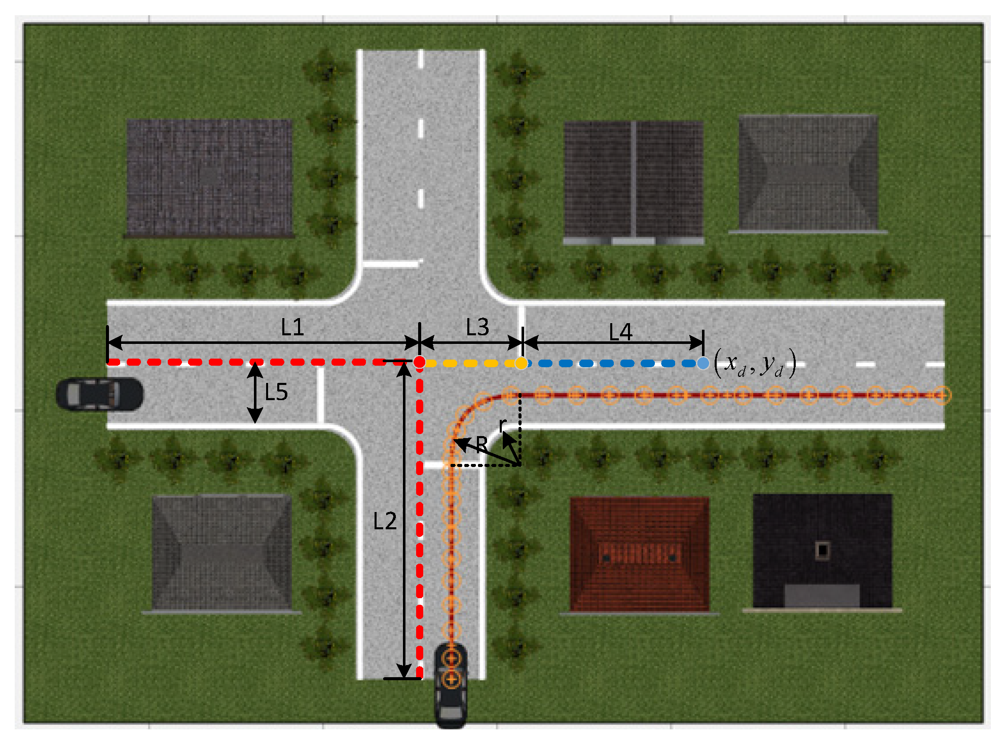
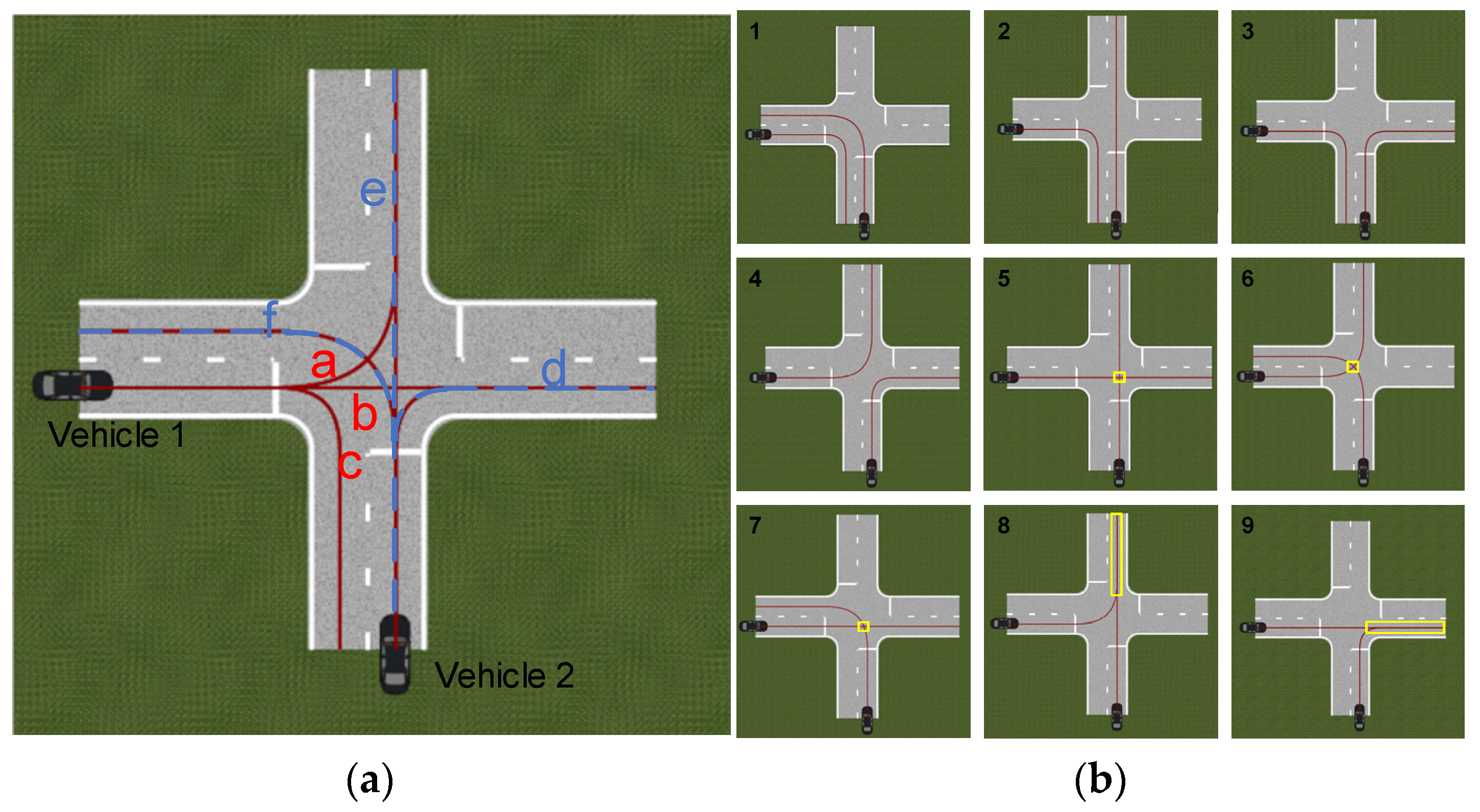
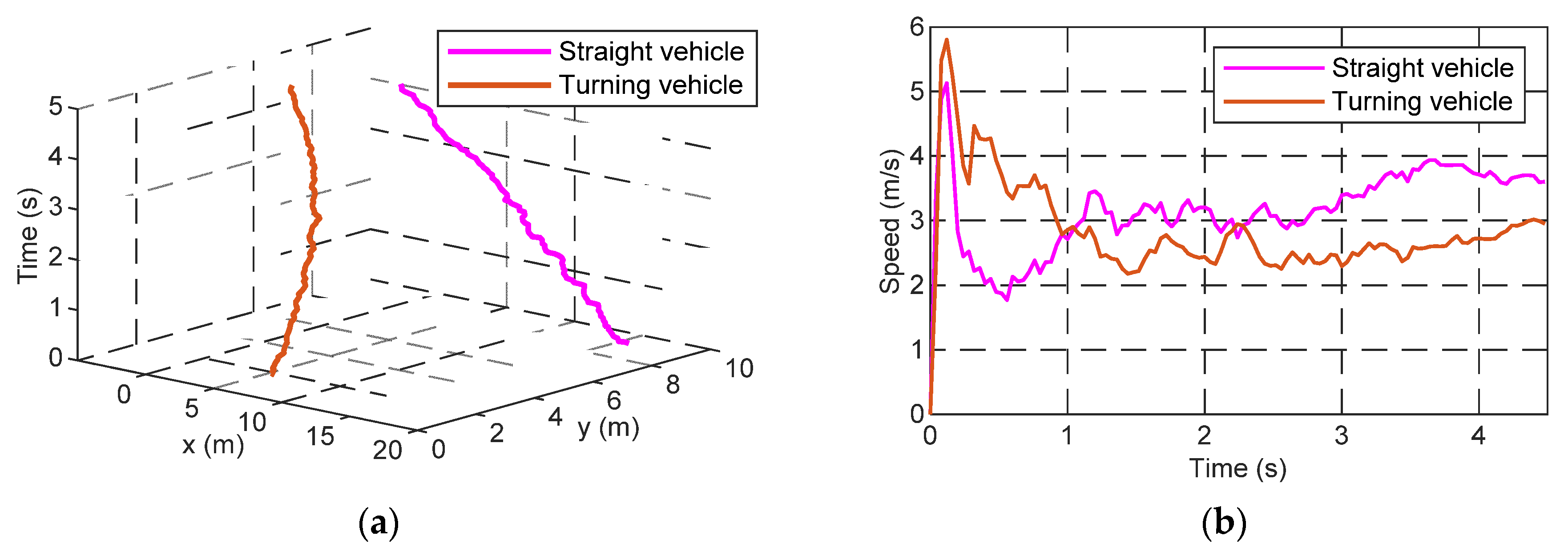
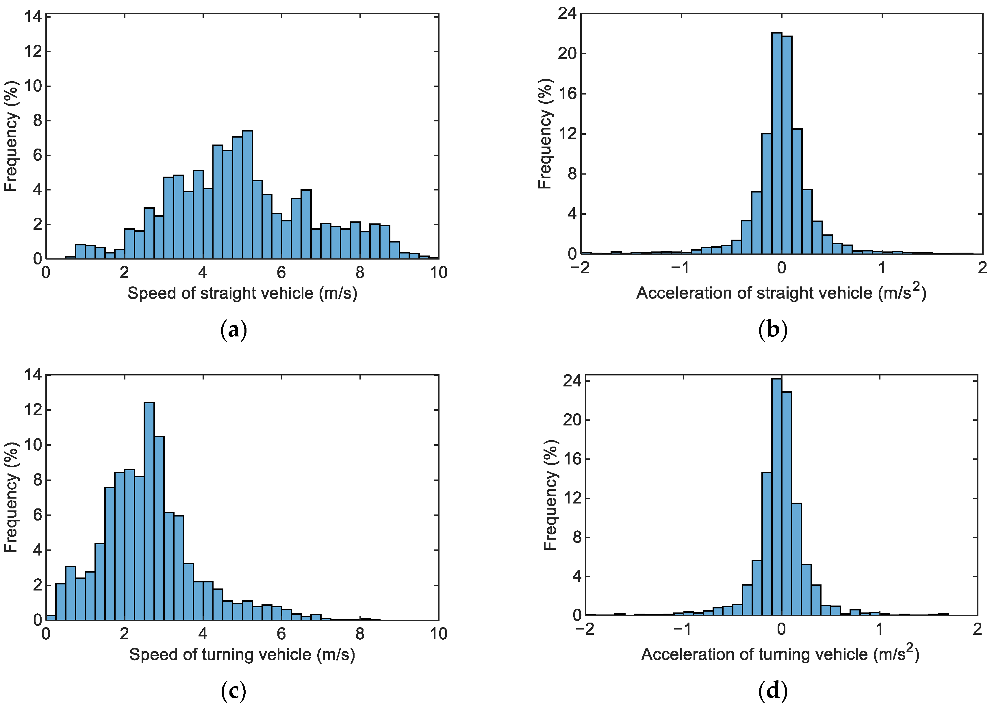
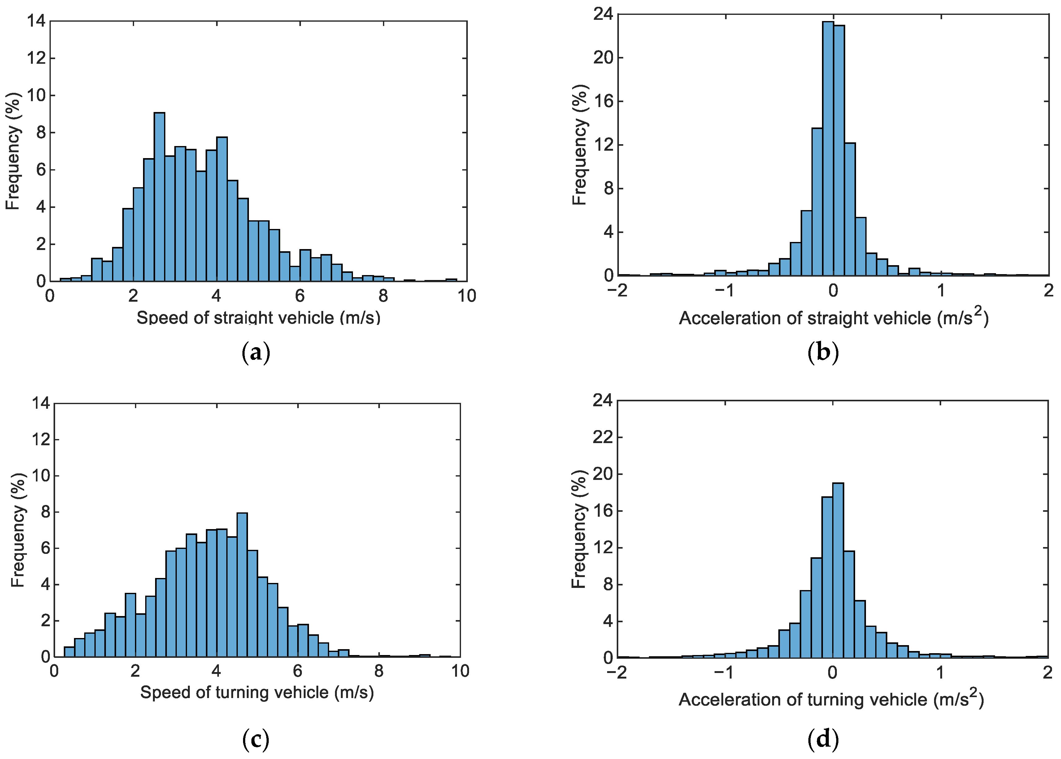
2.2. Statistical Analysis of Intersection Confluence Trajectory Data

To mimic the actual working conditions in this study, the intersection-trajectory dataset published by Open ITS [26] was imported to conduct the driving-behavior analysis at intersections. Open ITS is a traffic-data resource-sharing platform built jointly by different research institutes and enterprises. Open ITS provides trajectory data of intersections involving a total of 60 confluence conditions. Figure 7 shows one example of the dataset, which contains information about the position, speed, and acceleration change with time, of straight and turning vehicles.
A speed that is too high or too low at an intersection is dangerous, and as such it is necessary to determine the speed and acceleration threshold of vehicles driving through the intersection. Grouped statistics are made according to the passing order of vehicles going straight at intersections, and the statistical results are shown in Figure 8 and Figure 9, where Figure 8 shows the speed and acceleration distribution of straight and turning vehicles in the case of a straight vehicle going before a turning vehicle, and Figure 9 sketches the distribution when the straight vehicle gives way.
The statistical results reveal that under the two working conditions the velocity and acceleration are mainly distributed in a certain range. The vehicle speed is mainly distributed in the range of 0 to 8 m/s, and the acceleration is mainly distributed in the range of −2 to 2 m/s2, thereby providing a reference basis for boundary-condition setting.

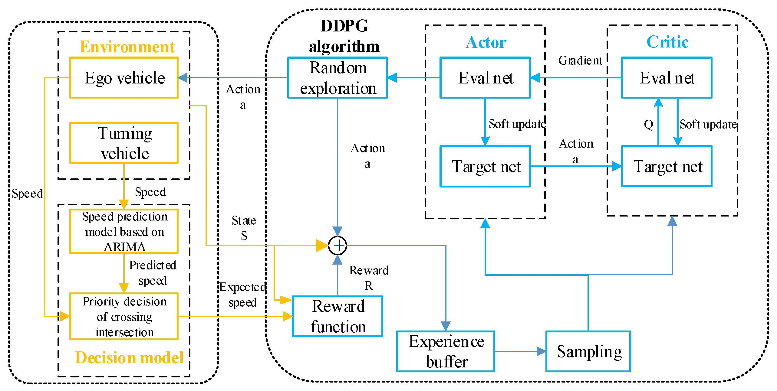
3. Decision Making and Control Based on RL and ARIMA Prediction

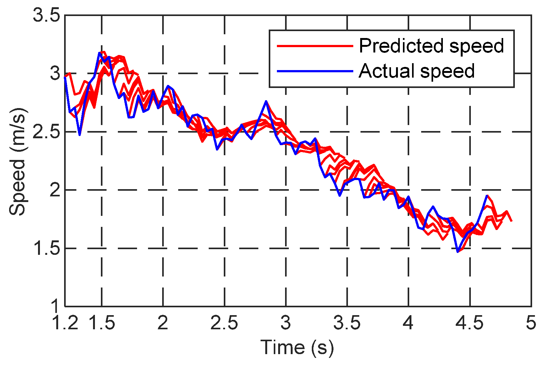
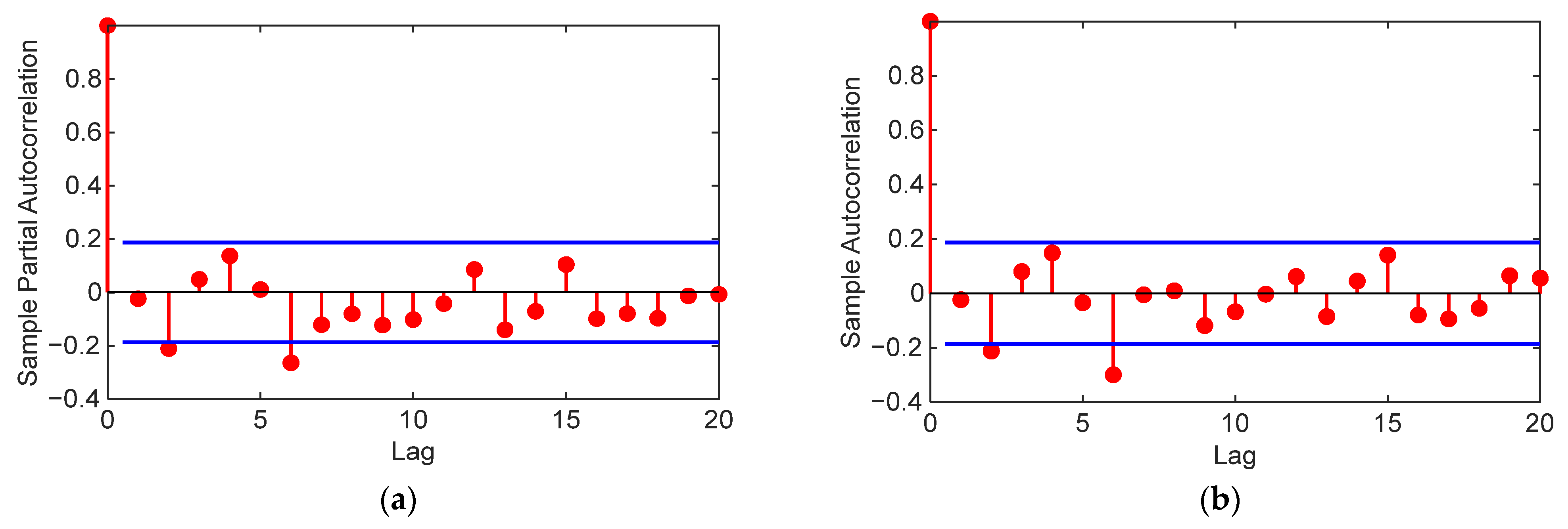
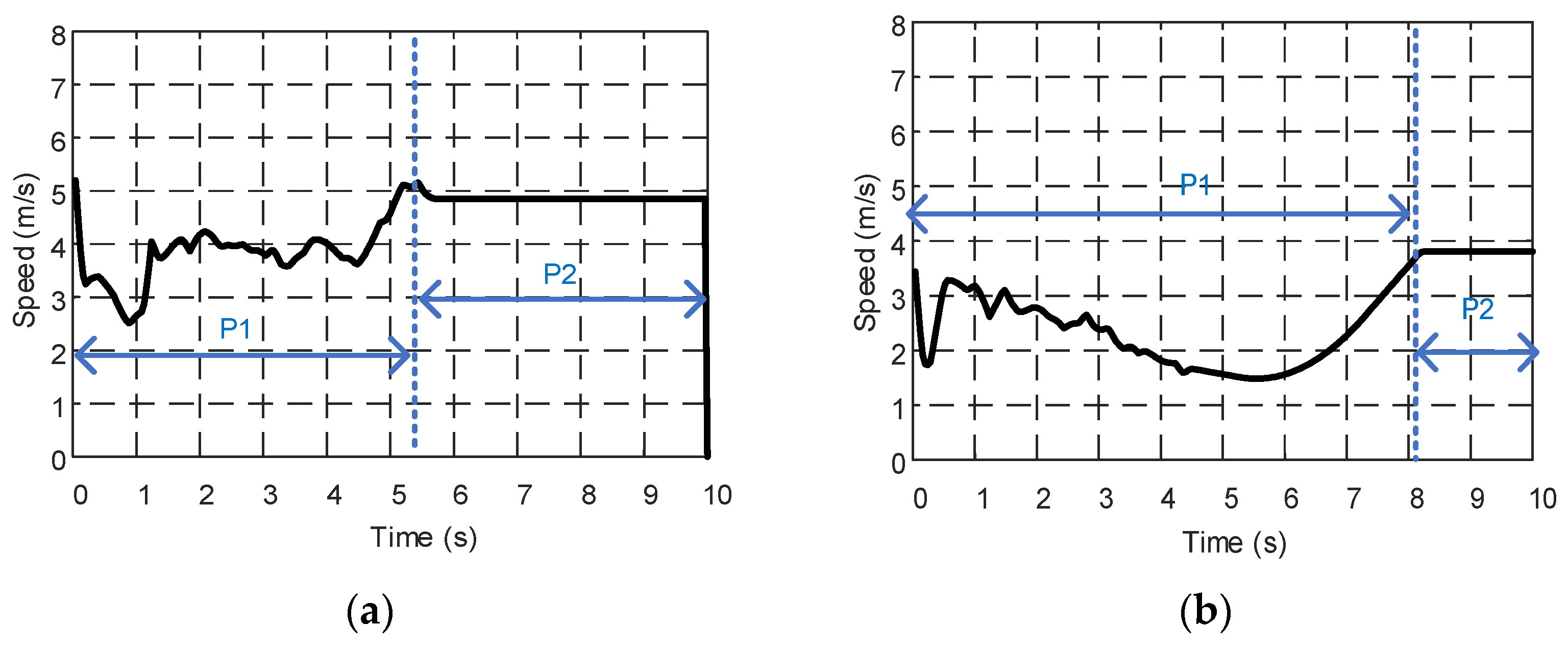
3.1. Turning-Vehicle Speed Prediction

Owing to the limited space and high risk of collision at the intersection, the state of vehicles in the surrounding environment should be predicted from the perspective of safety. Hence, the ARIMA model is considered to predict the future speed of the turning vehicle. Taking the confluence trajectory data from the first data group in the Open ITS dataset as an example, the inductive method based on the self-correlation function and partial self-correlation function is adopted to determine the order of the model [27]. The self-correlation function and partial self-correlation function are shown in Figure 10. As can be found, the second-order difference in the speed of the selected track data is a stationary time series. The blue line in the figure represents the 95% confidence interval. In general, the determination of the order of the ARIMA model is based on the last point outside the confidence interval. Therefore, in this study, both parameters of the second-order-difference ARIMA model of the turning vehicle can be set to 6.
With the established ARIMA speed-prediction model, the future speed of the turning vehicle can be predicted, providing information for the vehicle to decide to go ahead or give way to the turning vehicle at the intersection. The sampling step of speed in the data set is 0.04 s. In order to reduce the computing load of on-board processors and maintain accuracy and predictability, we set the predicted time to 0.2 s to predict the speed after five sampling steps. Figure 11 shows the result of speed prediction. The mean value of the actual vehicle speed is 2.331 m/s, while the mean square speed errors of the rolling prediction model in the next five steps are 0.0243, 0.0325, 0.0370, 0.0410, and 0.0411, respectively. Most of the mean square errors of speed prediction are approximately within 1%, and the maximum is less than 2%, demonstrating superior prediction performance.

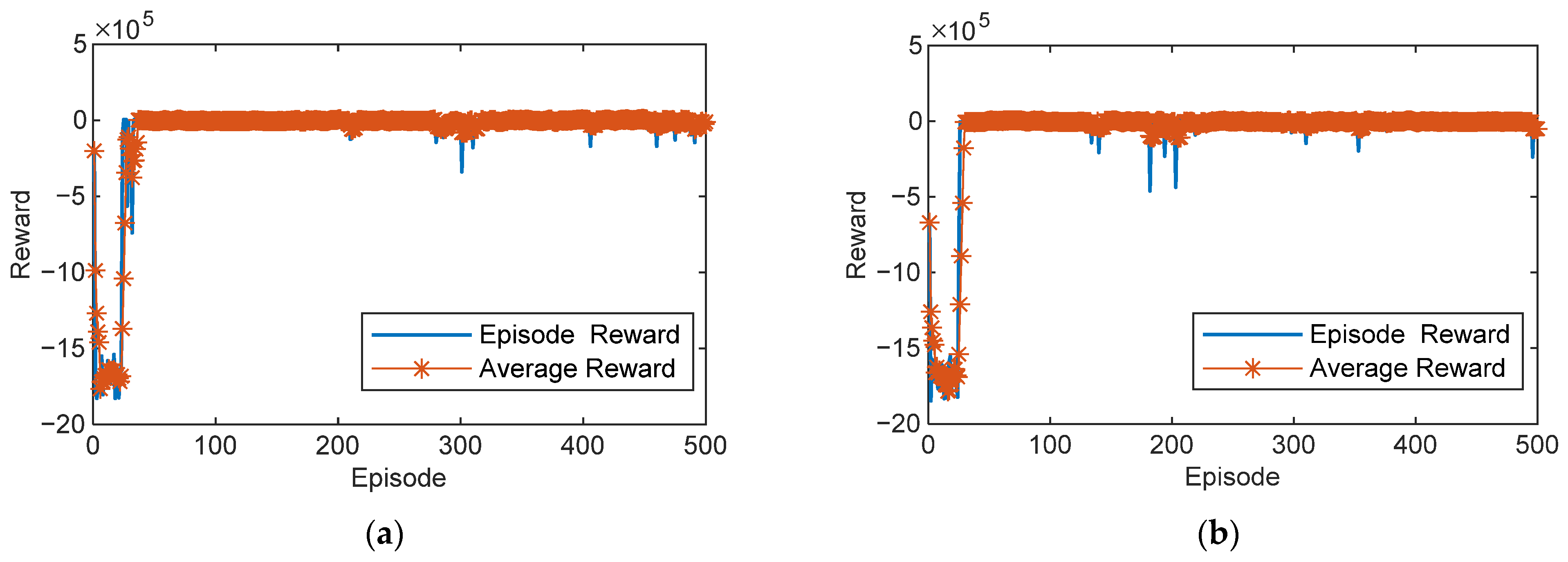
3.2. Decision and Control Based on RL

RL is commonly employed to solve problems with complex decisions and control. In the decision process, the tuples ( S , A , R , S ) represent the basic units of each training, in which S denotes the current state, S denotes the new state that transfers from S taken action A , and a reward R is received according to the actions and states. The proper state space and action space should be carefully constructed in RL for decision making by intelligent vehicles. The construction of the state space is mainly based on the position and speed information of the two vehicles, as shown in (3) to (5). In this paper, the subscript ego represents the ego vehicle, and the subscript env denotes the turning vehicle in the environment.
o b s e r v i s i o n = ( S e g o , S e n v ) T
S e g o = ( x e g o , y e g o , v e g o )
S e n v = ( x e n v , y e n v , v e n v )
where S e g o and S e n v denote the sequence of state of the straight vehicle and turning vehicle, respectively, and ( x , y , v ) denote the abscissa, ordinate, and velocity of the vehicle, respectively. As for the action space, a natural way is to set the action as the throttle percentage and brake-pedal pressure, which can simplify the design of the tracking controller. However, the simultaneous output of the above two actions leads to an unreasonable strategy, such as pressing the throttle and braking simultaneously. Thus, the action space illustrated in (6) to (8) is constructed to avoid the problem, in which A c t i o n _ m i x indicates the brake-pedal pressure or throttle opening of the vehicle, and its value range [ A c t i o n _ min , A c t i o n _ max ] is determined by simulation experiment according to the statistical results depicted in Figure 8 and Figure 9.
A c t i o n = A c t i o n _ m i x ( A c t i o n _ min A c t i o n _ m i x A c t i o n _ max )
T h r o t t l e = { A c t i o n _ m i x 0 A c t i o n _ m i x > 0 A c t i o n _ m i x 0
B r e a k p r e s s = { 0 A c t i o n _ m i x A c t i o n _ m i x > 0 A c t i o n _ m i x 0
The arrival time required for straight and turning vehicles from the current position to the three centers ( x , y ) , ( x 2 , y 2 ) , and ( x 1 , y 1 ) is shown in Figure 6 and can be calculated according to (9) to (15). For straight vehicles, the minimum time to arrive at the key position is calculated with the permitted maximum acceleration a max , which is 2 m/s2 in this study. Here, v p r e represents the prediction result of the ARIMA multistep speed-prediction model [ v p r e 1 , v p r e 2 , , v p r e l 1 , v p r e l ] , and l denotes the predicted length in five steps. In addition, the situation when the straight vehicle reaches the maximum speed v max before arriving at the key position is considered in (9) and (11), and v max is set to 8 m/s according to the conclusion of Section 2.2.
{ T e g o _ x = v max v e g o a max + S 1 ( v max 2 v e g o 2 ) / 2 a max v max v e g o 2 + 2 a max S 1 > v max 2 T e g o _ x = v e g o 2 + 2 a max S 1 a max v e g o 2 + 2 a max S 1 v max 2
S 1 = x x e g o
{ T e g o _ x 2 = v max v e g o a max + S 2 ( v max 2 v e g o 2 ) / 2 a max v max v e g o 2 + 2 a max S 2 > v max 2 T e g o _ x 2 = v e g o 2 + 2 a max S 2 a max v e g o 2 + 2 a max S 2 v max 2
S 2 = x 2 x e g o
T e n v _ y 1 = S 3 v p r e ¯
S 3 = y 1 y e n v
v p r e ¯ = v p r e l
If two vehicles driven by humans arrive at an intersection at different times, we should determine which vehicle should give way according to the “first-in, first-out” rule. If two vehicles arrive at an intersection at the same time, the traffic regulations stipulate that the straight vehicle has the right of way. However, due to the limitation of drivers, it is sometimes difficult for them to accurately judge the order of two vehicles arriving at the intersection; therefore, both vehicles will usually slow down and pass through the intersection sequentially, greatly affecting the traffic efficiency of the unsignalized intersection. Therefore, the following method is proposed to facilitate the safe and orderly movement of traffic. For security reasons, a straight vehicle should speed up and pass through the intersection if there is a certainty; otherwise, it should slow down appropriately to give way.
In this paper, the priority of crossing the intersection that we made is presented as follows: if the time for the straight vehicle arriving at ( x , y ) is less than that of the turning vehicle when reaching ( x 1 , y 1 ) , then the straight vehicle goes ahead. Otherwise, if the time for the straight vehicle to arrive at point ( x 2 , y 2 ) is longer than that for the turning vehicle to arrive at ( x 1 , y 1 ) , then the straight vehicle gives way to the turning vehicle. Consequently, according to the required time calculated before, the decision-making model should be established to output the decision of going ahead or giving way, and the RL agent can be instructed to learn and converge to the planned traffic strategy by calculating the expected acceleration. The expected speed of the intelligent vehicle can be computed using (16), where Δ t denotes the step interval between two decisions. The expected acceleration is calculated by (17), which considers the sequence of the two vehicles reaching the key position. Here, v min denotes the lower limit of the vehicle speed, and K 1 denotes the constant term of inverse proportion function—here set as 1—meaning that the acceleration of the straight vehicle is inversely proportional to the arrival-time difference between the two vehicles.
v r e f = v e g o + a r e f Δ t
{ a r e f = a min × v e g o v min v e g o T e n v _ y 1 < T e g o _ x 2 a r e f = min ( a max , K 1 T e n v _ y 1 T e g o _ x ) T e n v _ y 1 > T e g o _ x K 1 > 0 a r e f = a min × v e g o v min v e g o T e g o _ x 2 < T e n v _ y 1 < T e g o _ x
The mathematical model of the RL reward function determines the convergence direction of the agent during learning. To ensure the efficiency and security of crossing at the intersection, the reward function shown in (18) to (22) is constructed. This reward function consists of aspects in collision, speed, and the position of whether to reach the end point. In addition, it also includes the difference between the reference acceleration calculated by (17) and actual acceleration of the vehicle, which will guide the agent to converge to the direction of the decision-making model. Compared with other rewards, the reward of R f is smaller, thereby accelerating the convergence speed of the agent in the training process, while avoiding limiting the ability of the agent to explore.
R G = { 5000 x e g o > x d x e n v > x d 0 x e g o x d x e n v x d
R C = { 5000 c o l l s i o n = 1 0 c o l l s i o n = 0
R S = { 5000 v e g o > v u p p e r v e g o < v l o w e r 0 v l o w e r v e g o v u p p e r
R f = { 20 | a r e f a e g o | < 0.4 10 | a r e f a e g o | > 1 0 0.4 < | a r e f a e g o | < 1
R r e w a r d = R G + R C + R S + R f
where R G denotes the reward for reaching the end point, R C denotes the penalty of collision, R S represents the penalty for speeding or being too slow, and R f is the reward for actual speed close to reference speed. x d denotes the abscissa of the end point, and v u p p e r and v l o w e r denote the upper and lower limits of speed, respectively. A deep deterministic policy gradient (DDPG) algorithm is employed as the training algorithm of RL. The structure of DDPG is mainly composed of an actor network and a critic network. The actor network is mainly responsible for outputting actions according to the current state, and the critic network accounts for outputting the value of the state-action pair. The flowchart of the decision-and-control model at the intersection based on RL and speed prediction by ARIMA is shown in Figure 12.

3.3. Model-Evaluation Method

To analyze the control effect of the quantitative model, five indexes, including success rate, speed penalty, safety, traffic efficiency, and comfort are considered to evaluate the performance. The success rate of the intersection is calculated by (23), in which 0 and 100 points are scored according to whether the vehicle finally passes the terminal. The speed penalty is evaluated by (24), in which t 1 denotes the sum of the duration when the vehicle speed exceeds and goes below the desired speed range, and t 2 denotes the total time duration when the last vehicle passes the finish line. The minimum distance between two vehicles is adopted as the index to evaluate the driving safety of intelligent vehicles. According to the circular model of vehicle body established in Section 2, the risk of collision increases with the approach of two body circles. Hence, a distance of 1.5 times the radius of the body circle is reserved in this study, and is therefore defined as the optimal interval between the two vehicles. A longer or shorter distance out of the optimum is considered an unsatisfactory scenario. The maximum distance is defined as the distance between the initial positions of two vehicles. The assessment of traffic safety at the intersection is shown in (25), where D is the diameter of the body circle, L max is the distance between the coordinates of the initial positions of two vehicles, and d min represents the minimum distance between two vehicles in the running process. In combination with the intersection simulation scene model, L max can be calculated in a straightforward manner according to (26), in which L is the width of the vehicle model adopted, and L 1 represents the distance from the initial position of straight vehicle to the longitudinal centerline of the intersection, and L 2 represents the distance from the initial position of turning vehicle to the horizontal centerline of the intersection.
S G = { 100 g o a l = 1 0 g o a l = 0
S L = 100 × ( 1 t 1 t 2 )
S S = { 100 × ( 1 1.5 D d min 0.5 D ) d min 1.5 D 100 × ( L max d min L max 1.5 D ) d min > 1.5 D
L max = ( L 1 + 1 2 L ) 2 + ( L 2 1 2 L ) 2
The traffic efficiency of vehicles at intersections is usually calculated based on the time of crossing the intersection. This study evaluates the traffic efficiency of intelligent vehicles based on Equation (27), where T max and T min represent the time duration from T = 0 to the terminal under the condition that the vehicles accelerate or decelerate to the limited speed with the maximum permitted acceleration or deceleration, as expressed in (28) and (29), where v i n i , v u p p e r , and v l o w e r denote the initial speed, upper speed limit, and lower speed limit, respectively, and S denotes the distance from the initial position to the finish line.
S T = 100 × ( 1 T T min T max T min )
T max = v i n i v l o w e r a min + ( S v i n i 2 v l o w e r 2 2 a min ) / v l o w e r
T min = v u p p e r v l o w e r a max + ( S v u p p e r 2 v i n i 2 2 a max ) / v u p p e r
The vehicle-comfort evaluation is relatively complex. In this study, a test standard in [28] is adopted to evaluate the degree of comfort for vehicles in the intersection. The standard stipulates that the root mean square (RMS) value of weighted acceleration is utilized to evaluate the impact of vibration on human comfort and health. The detailed calculation can be described as follows. Given the acceleration sequence a ( t ) in the time domain, the weighted-acceleration time series a w ( t ) is obtained through the filtering network of the frequency-weighting function w ( f ) , as expressed in (31), and the RMS value of the weighted acceleration can be calculated according to (30).
a w = [ 1 T 0 T a w 2 ( t ) d t ] 2
where T denotes the analysis time of vibration.
According to [28], the frequency-weighting functions w ( f ) at different input points and directions of vibration are different. In this study, only the vibration caused by longitudinal acceleration is considered. Thus, the vibration on the seat back is selected as the input point for comfort study. The standard stipulates that the final result of RMS value of the total weighted acceleration should consider the weighting of all the directions in the axial system, of which the calculation is shown in (32). Since the influence of lateral and vertical vibration is ignored in this study, the RMS value of the total weighted acceleration is simplified to (33), and k x = 0.8 is obtained by a look-up table. The relationship between the RMS value of the total weighted acceleration and passenger comfort level specified in [28] is presented in Table 1. Six levels of comfort scoring that evaluate the comfort level from “no discomfort” to “extremely uncomfortable” are defined as 100, 80, 60, 40, 20, and 0 points. Accordingly, the driving comfort of the vehicle is evaluated according to the level of passenger comfort in Table 1.
w c ( f ) = { 1 ( 0.5 < f < 8 ) 8 / f ( 8 < f < 80 )
a v j ¯ = ( k x 2 a w x ¯ 2 + k y 2 a w y ¯ 2 + k z 2 a w z ¯ 2 ) 1 2
a v ¯ = k x a w x ¯
The overall comfort score is calculated by (34), in which S C ( i ) is the comfort score of each time period, and S C ( max ) represents the full score. After the scores of each evaluation index are calculated, the comprehensive score that evaluates the effect of decision making for the straight vehicle can be calculated by (35), where k i denotes the weight coefficient (0.2 in this study). The weight coefficient k i can be adjusted according to the needs of different scenarios. For instance, if passengers pay more attention to comfort and safety when crossing the intersection, but with no requirement for passing time, k 5 , k 3 can be increased and k 4 can be reduced.
S C = i = 1 10 S C ( i ) S C ( max )
S T o t a l = k 1 S G + k 2 S L + k 3 S S + k 4 S T + k 5 S C i = 1 5 k i = 1

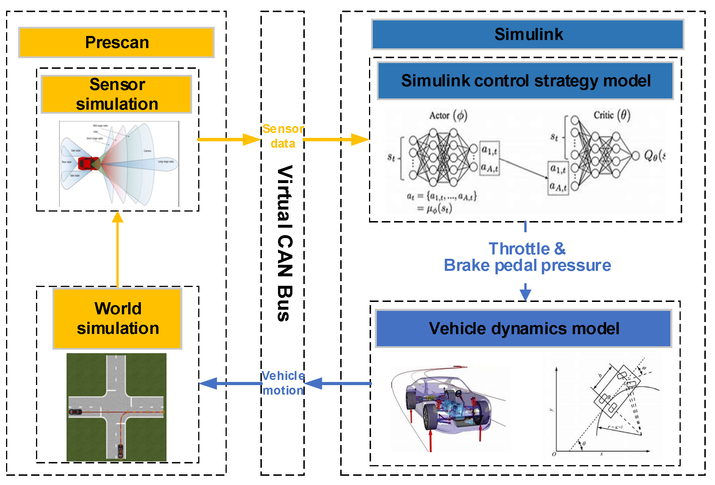
4. Validation and Discussion

In this study, sufficient traffic simulations are conducted to verify the effectiveness of the proposed method. The RL agent is trained using the proposed method under different driving conditions of intersections. Then, the simulation is performed to validate the effectiveness of decision making at the same initial speed. Finally, the overall performance of the proposed method is evaluated comprehensively with the indices mentioned in Section 3.3.

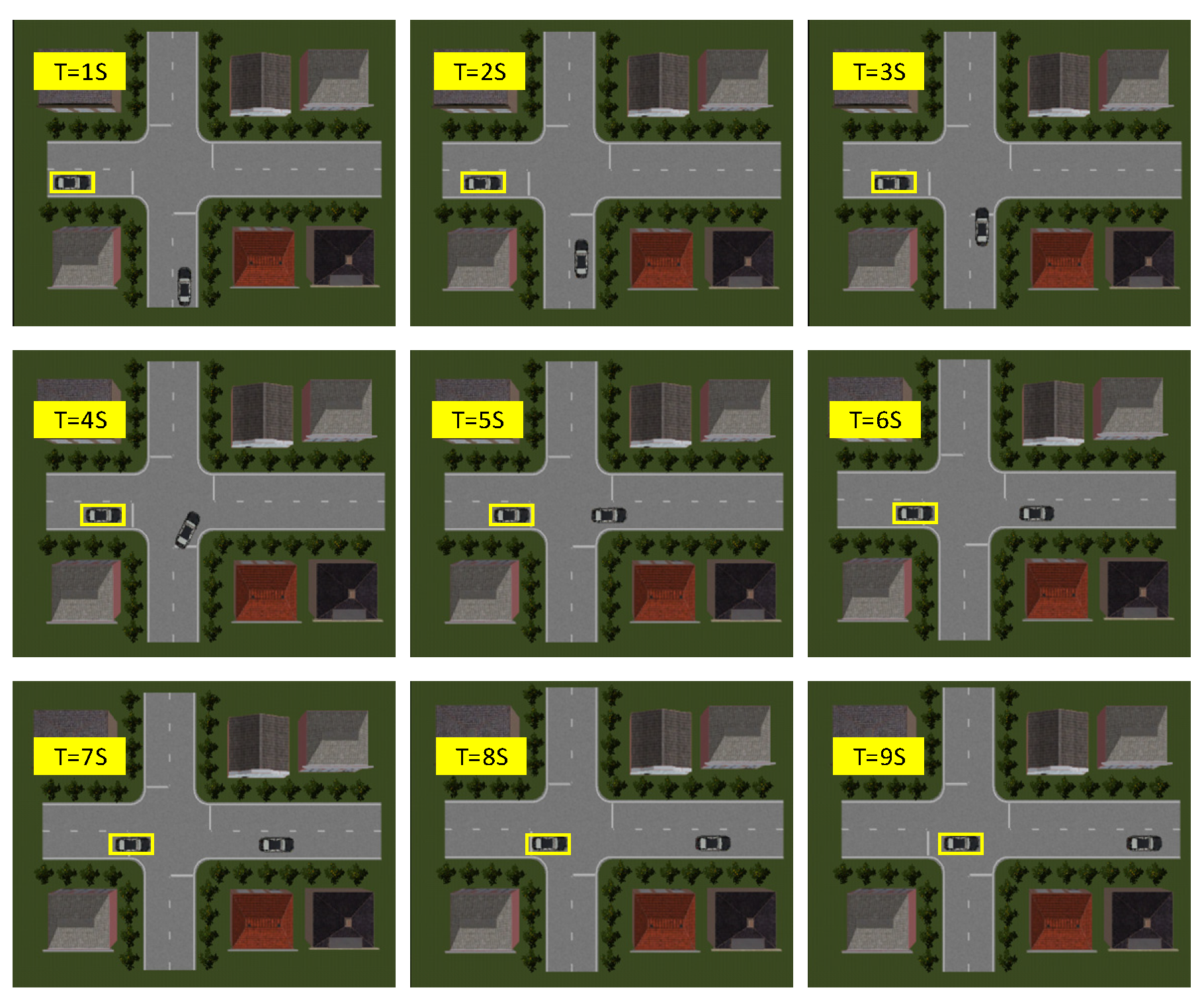
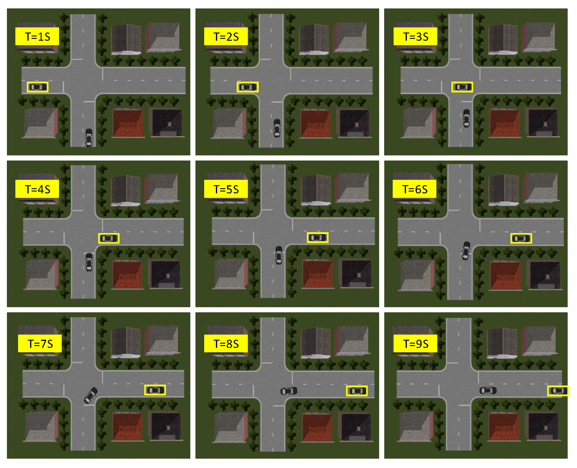
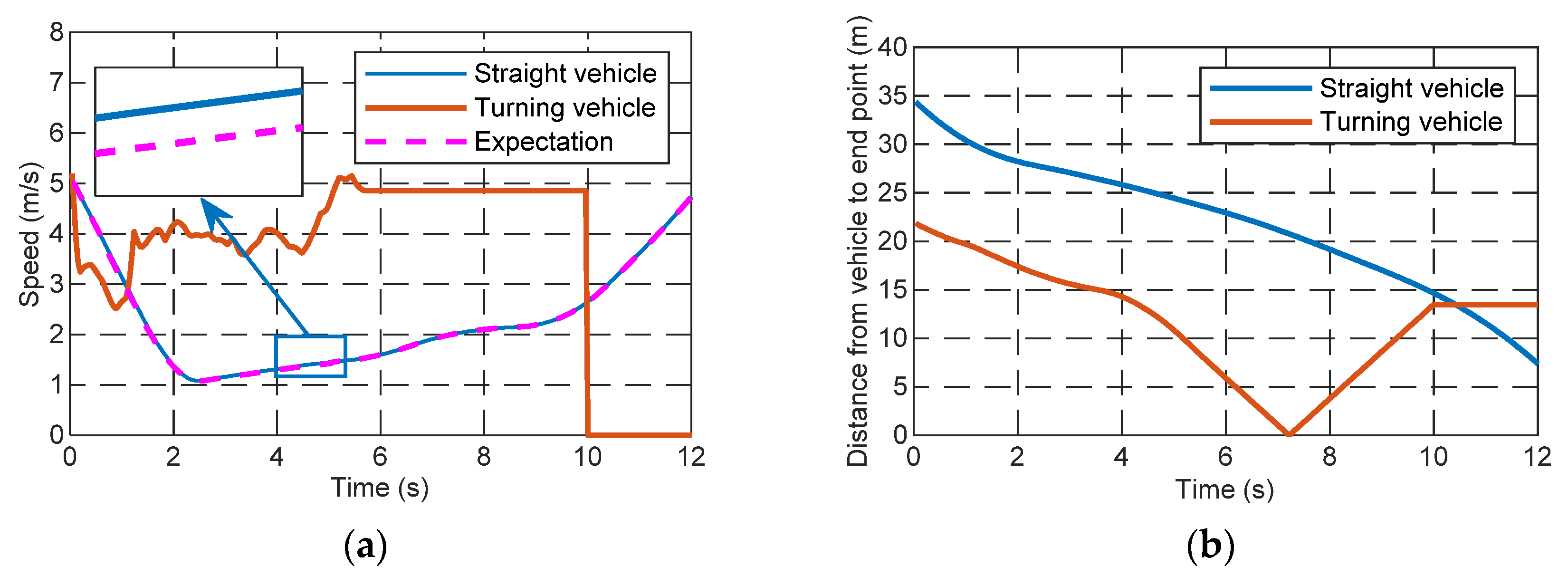
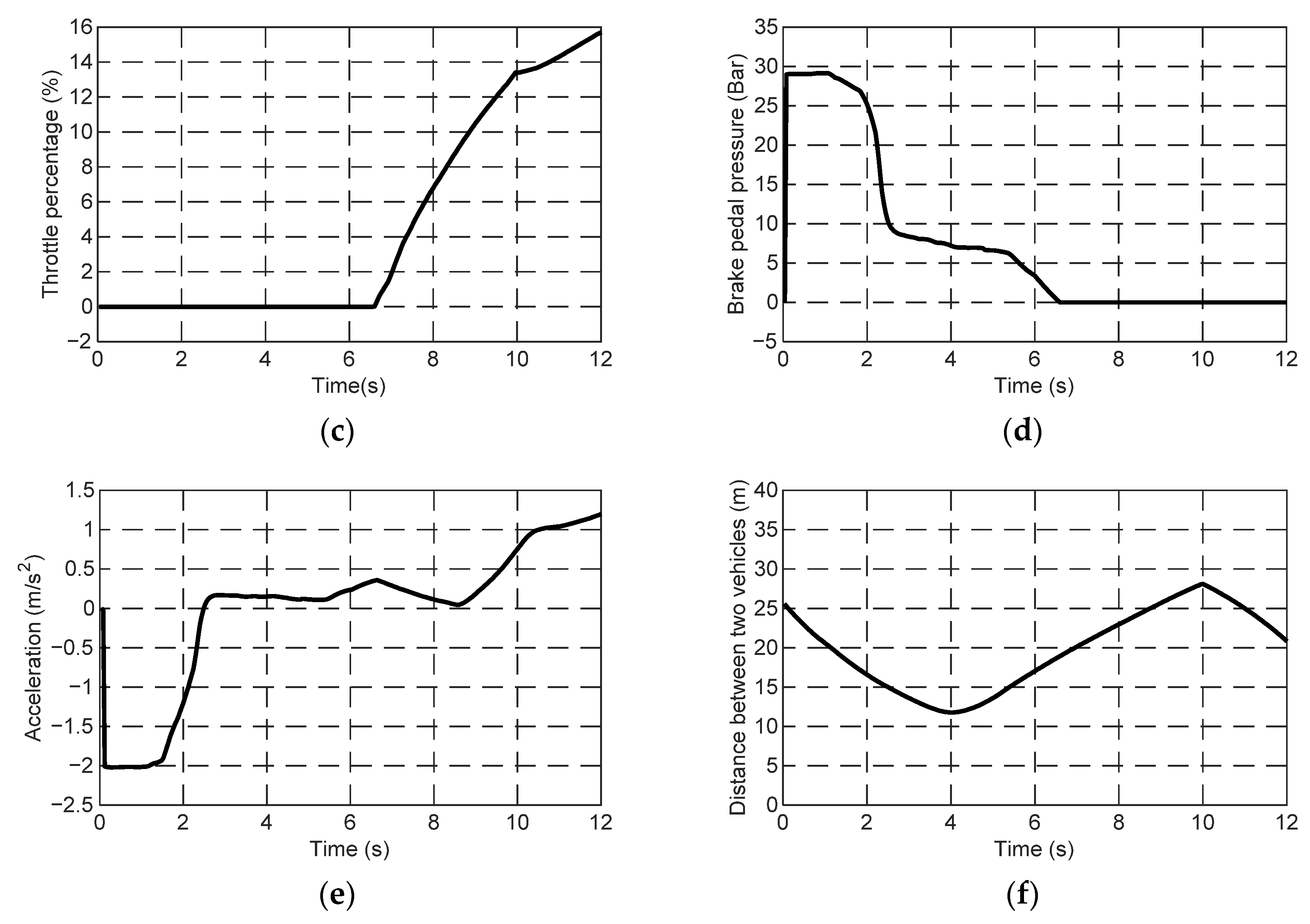
4.1. Simulation Validation

To verify the effectiveness of the proposed method, a number of cosimulation tests are carried out based on Prescan and Matlab/Simulink. In the simulation, Prescan is concerned with the provision of the intersection-simulation scene, and the vehicle information is exchanged between the Prescan and Simulink control models via a virtual CAN bus. A schematic diagram of the cosimulation process is shown in Figure 13.
Before the cosimulation, the scenario model of the road in the simulation should be constructed in Prescan, as shown in Figure 14. The specific values of parameters for each road segment are provided in Table 2.
The trajectory of the turning vehicle in the cosimulation condition is constructed based on the Open ITS dataset. The speed curve is shown in Figure 15, the related parameters in RL are shown in Table 3, and the reward convergence curve during the training process is shown in Figure 16.
The decision-making agent for a straight vehicle is obtained after RL training. In this study, verification experiments are conducted on the trained agents under two conditions to evaluate the control performance. To compare the effectiveness under different working conditions, the initial speeds of the agent in the experiments are kept the same. The speed range of the intersection is set from 0 to 8 m/s, and the initial speed of the vehicle in the verification experiment takes a middle value of 5 m/s within the allowable speed range.
The simulation results under condition I are shown in Figure 17a–f. The simulation results show that the straight vehicle slows down and gives way to the turning vehicle if the turning vehicle reaches the confluence point in advance. However, the straight vehicle still drives at a speed that is slightly higher than the lower speed limitation, rather than braking to stop. After the turning vehicle passes the confluence point on the road, the straight vehicle accelerates to follow the former vehicle as quickly as possible. In Figure 17a, the turning vehicle stops at the terminal of the intersection as the end of the trajectory of the turning vehicle is set at the terminal of the intersection. Figure 17b shows the distances to the terminal of the two vehicles. After passing the destination, the turning vehicle drives toward the end of the virtual scene, and this explains the trend of the speed curve that decreases first and then accelerates to the end. Moreover, no unreasonable strategy that leads to the conflict operation of the throttle and brake pedal can be found in Figure 17c,d, and the last two figures show that the acceleration and distance between the two vehicles are restricted under the limits of the entire process.
Figure 18 shows the simulation animation of the straight vehicle when it passes through the intersection under working condition I. The yellow rectangular area of the figure represents the straight vehicle that passes through the intersection; hence, the traffic priority of the two vehicles can be exhibited in the simulation animation.
The simulation results under working condition II are shown in Figure 19a–f and Figure 20. In working condition II, the speed of the turning vehicle is obviously lower than that of working condition I, and the straight vehicle on a straight road chooses to pass the intersection first. The simulation results show that the speed and acceleration of the intelligent vehicle in working condition II are also within the limitations.
As can be observed from the above simulation results, compared with the method proposed in [29] by sequential MDPs with standard or bipotential features, the proposed method can better smooth the speed curve of vehicles when passing through the intersection and promote the comfort performance. Since the lower limit of the speed is set, and the expected speed is leveraged to guide the agent, the parking at the intersection is effectively avoided, and the stop time at the intersection is also obviously reduced, compared with results presented in [29], thereby improving the traffic efficiency of the intersection.

4.2. Effect Evaluation

The above analysis verifies that the proposed controller is superior in decision making for the straight vehicle, and the trained agent can take the appropriate opportunity to pass the intersection encountering different turning vehicles. Since the simulation durations of working conditions I and II are inconsistent, the acceleration data from 0 to 10 s are selected to calculate the RMS value of weighted acceleration for the convenience of comparison. Owing to the fluctuations in the acceleration results, if the RMS of the weighted acceleration is calculated for the entire length of driving data, the comprehensive comfort evaluation concerning local acceleration fluctuation is intractable. Thus, the RMS of the weighted acceleration is calculated separately with 10 intervals from 0 to 10 s. The calculation results under the two working conditions are listed in Table 4 and Table 5, respectively, and the results are scored according to the scoring standard established in Section 3.3. The results show that the passenger comfort of the straight vehicle is worse at the beginning since the necessary acceleration or deceleration is inevitable to achieve the purpose of going ahead or giving way. After this stage, passenger comfort improves in the later confluence process.
Table 6 shows the comprehensive and individual scores of the indices of the proposed controller under the two conditions. For the success rate and speed penalty, in both conditions, the straight vehicle can successfully reach the ending point within the speed limit, and thus the scores of both items are 100 out of 100. For security, under working condition I, the minimum distance between two vehicles is always longer than the optimal interval, and they are relatively close. While the minimum distance between two vehicles under condition II is less than the optimal interval, thus the safety score under condition II is lower than that for condition I. In terms of traffic efficiency, the acceleration behavior of the straight vehicle under condition II according to the speed prediction of the steering vehicle makes the straight vehicle pass through the intersection ahead of the turning vehicle, which reduces the passage time, and as such it obtains a higher score in traffic efficiency, but at the expense of comfort. Based on the results above, the simulation results under the two working conditions can achieve preferable results in the comprehensive score. The results show that the proposed decision-control strategy can guide the vehicle to pass through an intersection safely and efficiently under different driving conditions.

5. Conclusions

To solve the decision-making and control problem at intersections for straight and turning vehicles, a decision-and-control method based on RL and vehicle-speed prediction is proposed. The road-geometry model of the intersection is built, and the distribution of speed and acceleration and the main factors that influence the decision process are analyzed based on an open-source confluence-trajectory dataset for intersections. Based on the ARIMA method, the speed prediction of the turning vehicle in the future time domain is conducted, and a decision-making method for intersections based on RL and ARIMA is proposed. Cosimulations are performed for the established intersection scene to validate the effectiveness of the proposed algorithm. The simulation results reveal that the trained RL agent can make appropriate decisions to pass the intersection safely and efficiently under two working conditions. Finally, the performance of the proposed method is evaluated based on the proposed evaluation standard from five indices. The results manifest that under different working conditions, the proposed method exhibits superior performance among all indices and comprehensive scores.
However, it is assumed that the sensing of the surroundings is precise and the traffic information can be received by the vehicle. The influence of errors caused by the perceptual layer should be addressed in the next research step. In addition, considering the multivehicle as agents, the interaction and game between vehicles also need to be further investigated.

Author Contributions

Conceptualization, Y.L. and Z.C.; methodology, G.L.; validation, G.L.; formal analysis, W.H.; investigation, Y.Z.; writing—original draft preparation, G.L.; writing—review and editing, Y.W., Y.L. and Z.C.; visualization, G.L.; supervision, Y.L. All authors have read and agreed to the published version of the manuscript.

Funding

This research was funded in part by the National Key R&D Program of China, grant number “2019YFE0121300” and in part by Foundation of State Key Laboratory of Automotive Simulation and Control, grant number “20201101”.

Data Availability Statement

The data presented in this study are available on request from the corresponding author.

Conflicts of Interest

The authors declare no conflict of interest. The funders had no role in the design of the study; in the collection, analyses, or interpretation of data; in the writing of the manuscript, or in the decision to publish the results.

References

  1. Shirazi, M.S.; Morris, B.T. Looking at Intersections: A Survey of Intersection Monitoring, Behavior and Safety Analysis of Recent Studies. IEEE Trans. Intell. Transp. Syst. 2017, 18, 4–24. [Google Scholar] [CrossRef]
  2. He, Y.; Yang, S.; Chan, C.Y.; Chen, L.; Wu, C. Visualization Analysis of Intelligent Vehicles Research Field Based on Mapping Knowledge Domain. IEEE Trans. Intell. Transp. Syst. 2021, 22, 5721–5736. [Google Scholar] [CrossRef]
  3. Zyner, A.; Worrall, S.; Ward, J.; Nebot, E. Long short term memory for driver intent prediction. In Proceedings of the 2017 IEEE Intelligent Vehicles Symposium (IV), Los Angeles, CA, USA, 11–14 July 2017; pp. 1484–1489. [Google Scholar]
  4. Noh, S. Decision-Making Framework for Autonomous Driving at Road Intersections: Safeguarding Against Collision, Overly Conservative Behavior, and Violation Vehicles. IEEE Trans. Ind. Electron. 2019, 66, 3275–3286. [Google Scholar] [CrossRef]
  5. Ma, L.; Xue, J.; Kawabata, K.; Zhu, J.; Ma, C.; Zheng, N. Efficient Sampling-Based Motion Planning for On-Road Autonomous Driving. IEEE Trans. Intell. Transp. Syst. 2015, 16, 1961–1976. [Google Scholar] [CrossRef]
  6. Ramyar, S.; Homaifar, A.; Anzagira, A.; Karimoddini, A.; Amsalu, S.; Kurt, A. Fuzzy modeling of drivers’ actions at intersections. In Proceedings of the 2016 World Automation Congress (WAC), Rio Grande, PR, USA, 31 July–4 August 2016; pp. 1–6. [Google Scholar]
  7. Hult, R.; Zanon, M.; Gros, S.; Falcone, P. Optimal Coordination of Automated Vehicles at Intersections: Theory and Experiments. IEEE Trans. Control Syst. Technol. 2019, 27, 2510–2525. [Google Scholar] [CrossRef]
  8. Zhao, X.; Wang, J.; Yin, G.; Zhang, K. Cooperative driving for connected and automated vehicles at non-signalized intersection based on model predictive control. In Proceedings of the 2019 IEEE Intelligent Transportation Systems Conference (ITSC), Auckland, New Zealand, 27–30 October 2019; pp. 2121–2126. [Google Scholar]
  9. Huang, L.X.; Panagou, D. Automated turning and merging for autonomous vehicles using a nonlinear model predictive control approach. In Proceedings of the 2017 American Control Conference (Acc), Seattle, WA, USA, 24–26 May 2017; pp. 5525–5531. [Google Scholar]
  10. Katriniok, A.; Kleibaum, P.; Josevski, M. Distributed Model Predictive Control for Intersection Automation Using a Parallelized Optimization Approach. IFAC Pap. 2017, 50, 5940–5946. [Google Scholar] [CrossRef]
  11. Schildbach, G.; Soppert, M.; Borrelli, F. A collision avoidance system at intersections using robust model predictive control. In Proceedings of the 2016 IEEE Intelligent Vehicles Symposium (IV), Gothenburg, Sweden, 19–22 June 2016; pp. 233–238. [Google Scholar]
  12. Bouton, M.; Cosgun, A.; Kochenderfer, M.J. Belief state planning for autonomously navigating urban intersections. In Proceedings of the 2017 IEEE Intelligent Vehicles Symposium (IV), Los Angeles, CA, USA, 11–14 June 2017; pp. 825–830. [Google Scholar]
  13. Shu, K.; Yu, H.; Chen, X.; Chen, L.; Wang, Q.; Li, L.; Cao, D. Autonomous driving at intersections: A critical-turning-point approach for left turns. In Proceedings of the 2020 IEEE 23rd International Conference on Intelligent Transportation Systems (ITSC), Rhodes, Greece, 20–23 September 2020; pp. 1–6. [Google Scholar]
  14. Kye, D.K.; Kim, S.W.; Seo, S.W. Decision making for automated driving at unsignalized intersection. In Proceedings of the 2015 15th International Conference on Control, Automation and Systems (Iccas), Busan, Korea, 13–16 October 2015; pp. 522–525. [Google Scholar]
  15. Hubmann, C.; Quetschlich, N.; Schulz, J.; Bernhard, J.; Althoff, D.; Stiller, C. A POMDP maneuver planner for occlusions in urban scenarios. In Proceedings of the 2019 IEEE Intelligent Vehicles Symposium (IV), Paris, France, 9–12 June 2019; pp. 2172–2179. [Google Scholar]
  16. Hubmann, C.; Schulz, J.; Becker, M.; Althoff, D.; Stiller, C. Automated Driving in Uncertain Environments: Planning With Interaction and Uncertain Maneuver Prediction. IEEE Trans. Intell. Veh. 2018, 3, 5–17. [Google Scholar] [CrossRef]
  17. Mnih, V.; Kavukcuoglu, K.; Silver, D.; Graves, A.; Antonoglou, I.; Wierstra, D.; Riedmiller, M. Playing Atari with Deep Reinforcement Learning. arXiv 2013, arXiv:1312.5602. [Google Scholar]
  18. Silver, D.; Huang, A.; Maddison, C.J.; Guez, A.; Sifre, L.; Van Den Driessche, G.; Schrittwieser, J.; Antonoglou, I.; Panneershelvam, V.; Lanctot, M.; et al. Mastering the game of Go with deep neural networks and tree search. Nature 2016, 529, 484–489. [Google Scholar] [CrossRef] [PubMed]
  19. Isele, D.; Rahimi, R.; Cosgun, A.; Subramanian, K.; Fujimura, K. Navigating occluded intersections with autonomous vehicles using deep reinforcement learning. In Proceedings of the 2018 IEEE International Conference on Robotics and Automation (ICRA), Brisbane, QLD, Australia, 21–25 May 2018; pp. 2034–2039. [Google Scholar]
  20. Shi, Y.; Liu, Y.; Qi, Y.; Han, Q. A Control Method with Reinforcement Learning for Urban Un-Signalized Intersection in Hybrid Traffic Environment. Sensors 2022, 22, 779. [Google Scholar] [CrossRef] [PubMed]
  21. Chen, W.; Lee, K.; Hsiung, P. Intersection crossing for autonomous vehicles based on deep reinforcement learning. In Proceedings of the 2019 IEEE International Conference on Consumer Electronics—Taiwan (ICCE-TW), Yilan, Taiwan, 20–22 May 2019; pp. 1–2. [Google Scholar]
  22. Zhou, M.; Yu, Y.; Qu, X. Development of an Efficient Driving Strategy for Connected and Automated Vehicles at Signalized Intersections: A Reinforcement Learning Approach. IEEE Trans. Intell. Transp. Syst. 2020, 21, 433–443. [Google Scholar] [CrossRef]
  23. Bucolo, M.; Buscarino, A.; Famoso, C.; Fortuna, L.; Frasca, M. Control of imperfect dynamical systems. Nonlinear Dyn. 2019, 98, 2989–2999. [Google Scholar] [CrossRef]
  24. Liu, Y.; Zhou, B.; Wang, X.; Li, L.; Cheng, S.; Chen, Z.; Li, G.; Zhang, L. Dynamic Lane-Changing Trajectory Planning for Autonomous Vehicles Based on Discrete Global Trajectory. IEEE Trans. Intell. Transp. Syst. 2021. [Google Scholar] [CrossRef]
  25. Xu, X.; Zuo, L.; Li, X.; Qian, L.; Ren, J.; Sun, Z. A Reinforcement Learning Approach to Autonomous Decision Making of Intelligent Vehicles on Highways. IEEE Trans. Syst. Man Cybern. Syst. 2020, 50, 3884–3897. [Google Scholar] [CrossRef]
  26. OpenITS. Available online: https://www.openits.cn/ (accessed on 13 January 2022).
  27. Tsay, R.S.; Tiao, G.C. Consistent estimates of autoregressive parameters and extended sample autocorrelation function for stationary and nonstationary ARMA models. J. Am. Stat. Assoc. 1984, 79, 84–96. [Google Scholar] [CrossRef]
  28. Method of Running Test—Automotive Ride Comfort. Available online: http://std.samr.gov.cn/gb (accessed on 13 January 2022).
  29. Yang, S.; Yoshitake, H.; Shino, M.; Shimosaka, M. Smooth and stopping interval aware driving behavior prediction at un-signalized intersection with inverse reinforcement learning on sequential MDPs. In Proceedings of the 2021 IEEE Intelligent Vehicles Symposium, Nagoya, Japan, 11–17 July 2021; pp. 586–593. [Google Scholar]
Figure 1. The relationship between two vehicles when passing through the intersection: (a) the possible driving directions of vehicle and (b) collision area under different conditions.
Electronics 11 01203 g001
Figure 2. Road-geometry model of intersection confluence condition.
Electronics 11 01203 g002
Figure 3. Circular model of vehicle body.
Electronics 11 01203 g003
Figure 4. Vehicle trajectory in confluence condition based on vehicle body circular method.
Electronics 11 01203 g004
Figure 5. The latent collision area of two vehicles.
Electronics 11 01203 g005
Figure 6. Vehicle body circles C1, C2, and C3 at the critical position.
Electronics 11 01203 g006
Figure 7. One example of Open ITS: (a) position of straight and turning vehicles, (b) acceleration of straight and turning vehicles.
Electronics 11 01203 g007
Figure 8. Statistical histogram of track information when the straight vehicle goes ahead: (a) speed of straight vehicle, (b) acceleration of straight vehicle, (c) speed of turning vehicle, and (d) acceleration of turning vehicle.
Electronics 11 01203 g008
Figure 9. Statistical-distribution histogram of track information when the straight vehicle gives way: (a) speed of straight vehicle, (b) acceleration of straight vehicle, (c) speed of turning vehicle, and (d) acceleration of turning vehicle.
Electronics 11 01203 g009
Figure 10. Analysis results after the second-order difference of the original velocity sample: (a) sample partial-autocorrelation function and (b) sample autocorrelation function.
Electronics 11 01203 g010
Figure 11. Speed-prediction results based on ARIMA model.
Electronics 11 01203 g011
Figure 12. The flowchart of decision-and-control model at intersection based on RL and speed prediction by ARIMA.
Electronics 11 01203 g012
Figure 13. Cosimulation schematic diagram for Simulink and Prescan.
Electronics 11 01203 g013
Figure 14. Scenario model in cosimulation.
Electronics 11 01203 g014
Figure 15. Speed curve of turning vehicle in cosimulation: (a) condition I and (b) condition II.
Electronics 11 01203 g015
Figure 16. Reward convergence of training process under different conditions: (a) condition I and (b) condition II.
Electronics 11 01203 g016
Figure 17. Simulation results of condition I: (a) vehicle velocity, (b) distance to destination, (c) throttle curve, (d) brake-press curve, (e) acceleration curve, and (f) distance between two vehicles.
Electronics 11 01203 g017aElectronics 11 01203 g017b
Figure 18. Simulation animation of condition I.
Electronics 11 01203 g018
Figure 19. Simulation results of condition II: (a) vehicle speed, (b) distance to destination, (c) throttle percentage, (d) brake-pedal pressure, (e) vehicle acceleration, and (f) distance between two vehicles.
Electronics 11 01203 g019
Figure 20. Simulation animation of condition II.
Electronics 11 01203 g020
Table 1. Relationship between the RMS value of the total weighted acceleration and passenger comfort level in [28].
RMS Value of Total Weighted AccelerationPassenger Comfort Level
<0.315No discomfort
0.315~0.63Little discomfort
0.5~1Some discomfort
0.8~1.6Uncomfortable
1.25~2.5More uncomfortable
>2Extremely uncomfortable
Table 2. Road model parameters in cosimulation.
ParameterDescriptionValue (m)
L 1 Distance from the initial position of straight vehicle to the center of the intersection18
L 2 Distance from the initial position of the turning vehicle to the center of the intersection18
L 3 Distance from road center to confluence point5.5
L 4 Distance from the point of confluence to the end of the confluence10.5
L 5 Road width3.5
R Radius of curvature at the turn of the road centerline4
r r o a d Radius of curvature at road edge bends2.25
Table 3. Related parameters in RL.
ParameterValue
Time duration of simulation16 s
Simulation step size0.04 s
Maximum number of training episodes500
Input-layer size6
Output-layer size1
Number of neurons144
Learning rate10−3
Discount factor0.9
Gradient threshold1
Experience-pool size106
Batch size64
Table 4. Calculation results of RMS of weighted acceleration when straight vehicle gives way.
Period of Acceleration (s)RMS of Weighted AccelerationPassenger ComfortScore
0–10.8890Some discomfort60
1–20.8131Some discomfort60
2–30.1932No discomfort100
3–40.0642No discomfort100
4–50.0540No discomfort100
5–60.0641No discomfort100
6–70.1522No discomfort100
7–80.0822No discomfort100
8–90.0194No discomfort100
9–100.2068No discomfort100
Table 5. Calculation results of RMS of weighted acceleration when straight vehicle goes ahead.
Period of Acceleration (s)RMS of Weighted AccelerationPassenger ComfortScore
0–10.5836Little discomfort80
1–20.6878Some discomfort60
2–30.8845Some discomfort60
3–40.5815Little discomfort80
4–50.4682Little discomfort80
5–60.3745Little discomfort80
6–70.2100No discomfort100
7–80.0510No discomfort100
8–90.6160Little discomfort80
9–100.2760No discomfort100
Table 6. Comparison of results for decision-control model under two driving conditions.
Working Condition IWorking Condition II
Success rate100100
Speed penalty100100
Security80.3570.04
Traffic efficiency65.6595.80
Passenger comfort9282
Comprehensive score87.6089.57
Publisher’s Note: MDPI stays neutral with regard to jurisdictional claims in published maps and institutional affiliations.

