Adaptive Fuzzy PID Control Strategy for Vehicle Active Suspension Based on Road Evaluation

Abstract

The paper proposes a fuzzy proportion integral differential (PID) control strategy based on road estimation to meet the different performance requirements of active suspension for comfort and safety under different road conditions in view of the uncertainty of vehicle suspension parameters and random road perturbations. First, flexible neural tree (FNT) is used to estimate the vertical disturbance of road within uncertain vehicle parameters in which the Fourier transform of the autocorrelation function is used to fit the road power spectrum density (PSD). In order to compensate for the delay and realize the real-time estimate of road conditions, an online fuzzy evaluation strategy for road condition is developed by integrating the fitted road PSD and the real-time suspension performance. After that, an adaptive fuzzy PID control strategy is developed based on the adaptive suspension control performance, which is supposed to realize the adaptive adjustment of control parameters for different road conditions. The simulation experimental results show that the online fuzzy evaluation strategy can effectively reflect the change in road condition, and the proposed adaptive fuzzy PID control strategy can work for adjusting the parameters adaptively, according to the changes in road conditions and therefore meet the control performance requirements under different road conditions.

1. Introduction

The suspension system, as an important component of the vehicle, connects the vehicle tires to the body by means of springs, damping and other components, which are used to reduce the impact of the road on the body, and increase the stability, safety and driving comfort of the vehicle. The existing vehicle suspension technology is mainly divided into passive suspension systems, semi-active suspension systems and active suspension systems. Passive suspension normally consists of springs and dampers, which, though simple and inexpensive, can only passively absorb energy and soften impacts [1]. Semi-active suspensions can change the suspension stiffness or damping parameters to improve the adaptability of the suspension under different road conditions [2]. The active suspension system, a combination of suspension control and vehicle status based on the information of the road and vehicle condition, relies on its own actuator to generate actuation forces between the vehicle and tires by following an active control strategy and adaptively generating adjustable suspension control forces, with the smoothness and handling stability of the vehicle [3] taken into account.

In response to the complexity of the suspension system as well as the external disturbances, adaptive control strategies have been widely adopted to devise active suspension control strategies, which are mainly two specific control methods: the online self-tuning control and the model reference adaptive control. The online self-tuning control is to change the parameters of the controlled object by means of online identified system parameter design rules [4], which can enhance the certain robustness under the condition of uncertainty and non-linearity of the system parameters. The model reference adaptive control evaluates the suspension performance in real time by using a reference model established in advance, and the results are used as the basis for adaptive adjustment [5]. Both control methods are effective in the evaluation of the suspension status, but require a mathematical model for the suspension system; however, the vehicle suspensions are frequently affected by wearing, spring load quality and other uncertainties.

To tackle the uncertainty of the suspension, fuzzy control is used in the active suspension control strategies with such characteristics as non-linearity and uncertainty. Li et al. [6] established a suspension model and fuzzified the suspension speed difference and suspension speed. They conducted a simulation experiment of fuzzy control, which showed that fuzzy control can effectively increase the stability and adjustment speed of the suspension. Na et al. [7] proposed a new adaptive fuzzy control scheme for active suspension systems, which can effectively control the stability of the vehicle in the case of time delay or uncertainty of suspension parameters. Although the fuzzy controllers have a low overshoot, strong robustness and the ability to overcome the non-linearity of the system, to improve the accuracy of fuzzy control still requires a greater number of quantization steps to increase the rule search range, reduce the decision speed and cope with the control under high motorization of vehicles [8]. Being able to deal with the conflicts between control accuracy and speed and to overcome the impact of uncertainties in the control parameters, the design of fuzzy PID control strategies for active vehicle suspensions has attracted widespread attention [9]. The fuzzy PID controller automatically adjusts the PID parameters online to suit the operating environment and the changing system parameters by using fuzzy inference decisions from system errors and changes in external excitation [10]. Yang [11] modeled a 1/4 semi-active suspension system and adopted fuzzy PID control, in which the velocity and acceleration in the vertical direction of the body are fuzzified as input quantities, achieving excellent control performance. Xu [12] linearized the active suspension system and fuzzed the body vertical speed error and the change rate of error to design a fuzzy PID controller, which enables the suspension system to have higher performance in driving comfort. Although the above methods contribute greatly to the accuracy and adaptability for the suspension control, they only overcome the uncertainty within their own parameters but are not adaptable to external excitations without actively pre-adjusting the control parameters to respond quickly to changes in external excitations.

The main role of the vehicle suspension is to eliminate the body vibration caused by irregular excitation of the road. Obtaining accurate road input can provide feedforward information for the control strategy design of suspension vibration damping. As for high-mobility vehicles, traditional contact measurements fail to provide online detection of the road [13]. Inertial profilers and LIDAR can be used to detect the road and obtain time–domain information in real time. Papadimitrakis et al. [14] proposed a road preview model predictive controller that introduced radial signals, used LiDAR to predict the road ahead, and proposed a predictive control scheme for the whole vehicle active suspension system. The accuracy of measurement is high; however, the cost of the system sensors is relatively high, and the accuracy is susceptible to the influence of the external environment, such as the weather [15]. In recent years, scholars have conducted research of the measurement of road roughness based on the suspension response, in which the suspension response is obtained by means of onboard sensors, such as acceleration sensors or dynamic displacement sensors. For example, Qin et al. [16] proposed a road classification strategy based on the acceleration measurement of unsprung mass, which combines the frequency domain classifier of random forest with the classifier of road PSD to achieve road classification with few sensed data. Dong et al. [17] proposed a FNT-based road classifier, which employs sliding windows to extract road features to improve the classification accuracy. A control method using state predictors was also proposed in [18], in which Kalman filters are used to estimate road types in order to switch between energy-saving and high-performance control modes. Liu et al. [19] proposed a method for the online estimation of road profile lines based on the dynamic response of vehicles. They used the transmission characteristics of the system to estimate road disturbances, and calculate the power spectrum to evaluate the road roughness. The above methods consider the impact of the non-linearity of the vehicle suspension model and its parametric time-varying characteristics on road detection, and use a sliding window to improve the robustness of the road detection against changes in body parameters. However, significant time delays in detection results appear when road conditions change significantly, which will inevitably weaken control performance.

Considering the aforementioned problems, this paper designs a fuzzy PID vehicle active suspension control strategy based on road detection to effectively cope with road changes and improve the performance of vibration damping, oriented to the uncertainty of suspension parameters and random disturbance of road. The main contributions of this paper are as follows:

(1)

A FNT-based road PSD fitter is proposed, considering the vehicle parameter uncertainty. A sampling window is introduced to train the FNT structure and parameters by using different vehicle speeds, sprung masses and the outputs of the semi-active suspension system as inputs to the FNT for obtaining information of road vertical disturbance estimation; the road PSD is fitted by Fourier transform with the autocorrelation function. This road PSD fitter has a simple network structure that provides fast and accurate road information for control strategy design.

(2)

A strategy for online road condition fuzzy evaluation is worked out by combining road spectral density fitting values and real-time suspension performance with the intention to compensate effectively the time delay caused by road PSD fitting and achieve online evaluation of road conditions.

(3)

An adaptive fuzzy PID damping control strategy is developed. The adaptive control strategy is introduced to weigh the different performance requirements of vehicle suspension for driving safety and comfort under different road conditions; the fuzzy PID vibration damping control strategy is devised based on this to realize the adaptive adjustment of control parameters for road conditions and control performance changes.

The rest of this paper is organized as follows. The road model and active suspension model are constructed, and the general framework and objectives of the control strategy design are presented in Section 2. A FNT-based road PSD fitter is designed in Section 3. An adaptive fuzzy PID control strategy for the active suspension system is devised in Section 4. The effectiveness of the designed adaptive fuzzy PID control strategy is verified in a simulation environment in Section 5. Conclusions are given in Section 6.

2. Problem Description

2.1. Random Road Disturbance

Random road disturbances directly affect the dynamic performance of active suspension systems. For real roads, the road roughness function $q\left(I\right)$ is a random function defined as the variation of the relative height q of the road to the baseline level and along the road alignment I with a mean value of zero and following a normal distribution.

The time domain disturbance curves are different under different road conditions and generally described in the form of road PSD. The road PSD $G_q\left(n\right)$ can be expressed by fitting the following equation [20]:

$$G_q\left(n\right)=G_q\left(n_0\right){\left(\frac{n}{n_0}\right)}^{-W}=G_q\left(n_0\right){n_0}^W\frac{v}{f^W},$$

(1)

where n is the number of waves contained in each meter, called the spatial frequency; $n_0$ is the reference spatial frequency; $G_q\left(n_0\right)$ is the value of the road spectrum at the reference spatial frequency, called the road roughness factor; and W is the frequency factor, generally set as 2.

According to the power spectral density characteristics of the road vertical velocity, a time–domain road roughness model can be simulated with the white noise method. Assuming that $w\left(t\right)$ is a Gaussian white noise with unit intensity of 1, $Z_r\left(t\right)$ is the vertical displacement of the road, and the vehicle speed v is a constant value, the simulated time–domain model of the road disturbance is defined as

$${\dot{z}}_r\left(t\right)=2\pi n_0\sqrt{G_q\left(n_0\right)v}w\left(t\right).$$

(2)

In order to make the road power spectrum approach follow the actual road conditions, the lower cut-off time frequency $f_0$ can be introduced on the basis of the road model. The improved road excitation model is given as

$${\dot{z}}_r\left(t\right)=2\pi n_0\sqrt{G_q\left(n_0\right)v}w\left(t\right)-2\pi n_{1}v{z}_r\left(t\right),$$

(3)

where $n_1=0.01$ m${}^{-1}$ is the cutoff spatial frequency under road roughness.

2.2. Dynamic Model of Active Suspension

For the vertical vibration caused by an uneven road, the 1/4 active suspension model is chosen as the control model in this case, and the architecture is shown in Figure 1. In this model, the sprung and unsprung masses are denoted as $m_s$ and $m_u$, respectively. The suspension system is described by a linear spring with a stiffness factor $k_s$ and a linear damper with a damping factor $c_s$. The tire is described by a linear spring with a vertical stiffness factor $k_t$ and a linear damper with a damping factor $c_t$. The active control force is generated by the actuator u.

As the tires stay in contact with the road, the differential equation for the dynamics of the 1/4 active linear suspension system is established based on Newton’s laws of motion, which is described as

$$\begin{array}{c}{\ddot{z}}_s\left(t\right)=\frac{k_s}{m_s}(z_{\mathrm{u}}\left(t\right)-z_s\left(t\right))+\frac{c_s}{m_s}({\dot{z}}_{\mathrm{u}}\left(t\right)-{\dot{z}}_s\left(t\right))+\frac{1}{m_s}u\left(t\right)\hfill \\ {\ddot{z}}_u\left(t\right)=\frac{-k_s}{m_u}(z_{\mathrm{u}}\left(t\right)-z_s\left(t\right))+\frac{-c_s}{m_u}({\dot{z}}_{\mathrm{u}}\left(t\right)-{\dot{z}}_s\left(t\right))+\frac{k_t}{m_u}(z_r\left(t\right)-z_u\left(t\right))+\frac{c_t}{m_u}({\dot{z}}_r\left(t\right)-{\dot{z}}_u\left(t\right))-\frac{1}{m_u}u\left(t\right)\hfill \end{array},$$

(4)

Meanwhile, control performance is selected as

$${\overline{y}}_c\left(t\right)=\left[\begin{array}{c}{\overline{y}}_{c1}\left(t\right)\hfill \\ {\overline{y}}_{c2}\left(t\right)\hfill \\ {\overline{y}}_{c3}\left(t\right)\hfill \end{array}\right]=\left[\begin{array}{c}\begin{array}{c}{\dot{z}}_s\left(t\right)\\ z_u\left(t\right)-z_s\left(t\right)\end{array}\hfill \\ z_r\left(t\right)-z_u\left(t\right)\hfill \end{array}\right].$$

(5)

The performance indicators to be considered in the design of the active suspension system include the passenger comfort, the road grip of the vehicle tires, and the suspension wear consumption. The passenger comfort is related to the vertical speed of the sprung mass ${\dot{z}}_s\left(t\right)$. The grip of the tires has a strong correlation with driving safety, where grip is reflected by the tires’ dynamic deflection $z_u\left(t\right)-z_r\left(t\right)$, and the suspended deflection $z_s\left(t\right)-z_u\left(t\right)$ affects the ride comfort and the wear of the suspension system, where excessive extension of the suspension accelerates the wear of the suspension system and also seriously affects the ride comfort. The suspension dynamic deflection and suspension speed were selected as measurement indicators, considering the physical realizability, as they reflect the dynamic performance of the vehicle and facilitate the setup of sensors with the acquisition of indicators. The observed outputs are defined as

$${\overline{y}}_m\left(t\right)=\left[\begin{array}{c}{\overline{y}}_{m1}\left(t\right)\hfill \\ {\overline{y}}_{m2}\left(t\right)\hfill \end{array}\right]=\left[\begin{array}{c}{z}_u\left(t\right)-z_s\left(t\right)\\ {\dot{z}}_s\left(t\right)\end{array}\right].$$

(6)

Notice that the system output $y_m$ is affected by road disturbances and vehicle suspension parameters, specifically vehicle driving speed, $m_s$ and $m_u$.

When fitting road disturbances on the basis of $y_m$, the effect of the vehicle suspension parameters should be fully considered. To establish the state–space equations, the state variables are selected

$$\overline{x}={[(z_u-z_s),{\dot{z}}_s,(z_r-z_u),{\dot{z}}_u]}^T.$$

(7)

Thus the continuous-time vehicle suspension system can be expressed as

$$\left\{\begin{array}{c}\dot{\overline{}}x\left(t\right)=\overline{A}\overline{x}\left(t\right)+\overline{B}u\left(t\right)+\overline{D}v\left(t\right)\hfill \\ {\overline{y}}_c=C\overline{x}\left(t\right)\hfill \\ {\overline{y}}_m=\overline{C}\overline{x}\left(t\right)\hfill \end{array}\right..$$

(8)

where

$$\begin{array}{c}\overline{A}=\left[\begin{array}{cccc}0& -1& 0& 1\\ \frac{k_s}{m_s}& -\frac{c_s}{m_s}& 0& \frac{c_s}{m_s}\\ 0& 0& 0& -1\\ -\frac{k_s}{m_u}& \frac{c_s}{m_u}& \frac{k_t}{m_u}& -\frac{c_t}{m_u}-\frac{c_s}{m_u}\end{array}\right],\overline{B}=\left[\begin{array}{c}0\\ \frac{1}{m_s}\\ 0\\ -\frac{1}{m_u}\end{array}\right],\overline{D}=\left[\begin{array}{c}0\\ 0\\ 1\\ \frac{c_t}{m_u}\end{array}\right],\hfill \\ C=\left[\begin{array}{cccc}0& 1& 0& 0\\ 1& 0& 0& 0\\ 0& 0& 1& 0\end{array}\right],\overline{C}=\left[\begin{array}{cccc}1& 0& 0& 0\\ 0& 1& 0& 0\end{array}\right].\hfill \end{array}$$

Assuming that the system sampling period is T, according to the Equation (7), we can obtain

$$x\left((k+1)T\right)=e^{\overline{A}T}x\left(kT\right)+\left({\int }_0^T{e}^{\overline{A}t}\overline{B}dt\right)u\left(kT\right)+\left({\int }_0^T{e}^{\overline{A}t}\overline{D}dt\right)v\left(kT\right).$$

(9)

The discrete model of the active suspension is

$$\left\{\begin{array}{c}x(k+1)=Ax\left(k\right)+Bu\left(k\right)+Dv\left(k\right)\hfill \\ y_c=Cx\left(k\right)\hfill \\ y_m=\overline{C}x\left(k\right)\hfill \\ x\left(0\right)=x_0\hfill \end{array}\right.,$$

(10)

where $x\left(k\right)$, $u\left(k\right)$, and $v\left(k\right)$ represent the state variables of the discrete active suspension system, the control input and the road excitation input, respectively; $A=e^{\overline{A}T}$, $B={\int }_0^T{e}^{\overline{A}t}\overline{B}dt$, $D={\int }_0^T{e}^{\overline{A}t}\overline{D}dt$.

2.3. Control Targets and General Framework

The main target of this study is to design an adaptive fuzzy PID controller to respond quickly to the different performance requirements for driving comfort and safety under different road conditions by effectively combining road information and suspension status to improve the performance of the system in terms of vibration damping and stability. The control architecture consists of two parts: the road PSD fitting part and the active suspension adaptive fuzzy PID control strategy. The general framework is shown in Figure 2.

Notice that the main advantage of this framework is to use road grade recognition and body state as fuzzy.

The main purpose of the road power spectral density fitting section is the provision of essential information of the road conditions ahead for the suspension damping control strategy. Firstly, the sensor receives the suspension response signal from the front half of the semi-active suspension system. Then, the signal is used as an input to the FNT together with the vehicle parameters to fit the vertical disturbance of the road. Finally, the vertical disturbance is used as an input to obtain the road power spectral density by means of a Fourier transformation on a self-consistent function.

The latter part is combined with the PSD fitting results of the former part to prejudge the road conditions and adopt different control objectives for different roads. Firstly, the results of road power density estimate and suspension online performance evaluation are fuzzified to obtain online fuzzy evaluation of road condition, which will adjust the control objective of the controller. Then the fundamental domain is adaptively adjusted by the real-time suspension displacement signal of the vehicle, which adjusts the road surface of different variation range to the same range. Finally, the performance deviation and its rate of change are fuzzified, and fuzzy rules are designed to realize the real-time adaptive adjustment of PID parameters, so that the controller can produce a control force to achieve different control effects on different road surfaces and the suspension system can quickly adapt to the internal response of the vehicle and the external changing road excitation.

3. FNT-Based Algorithm for Road Power Spectral Density Fitting

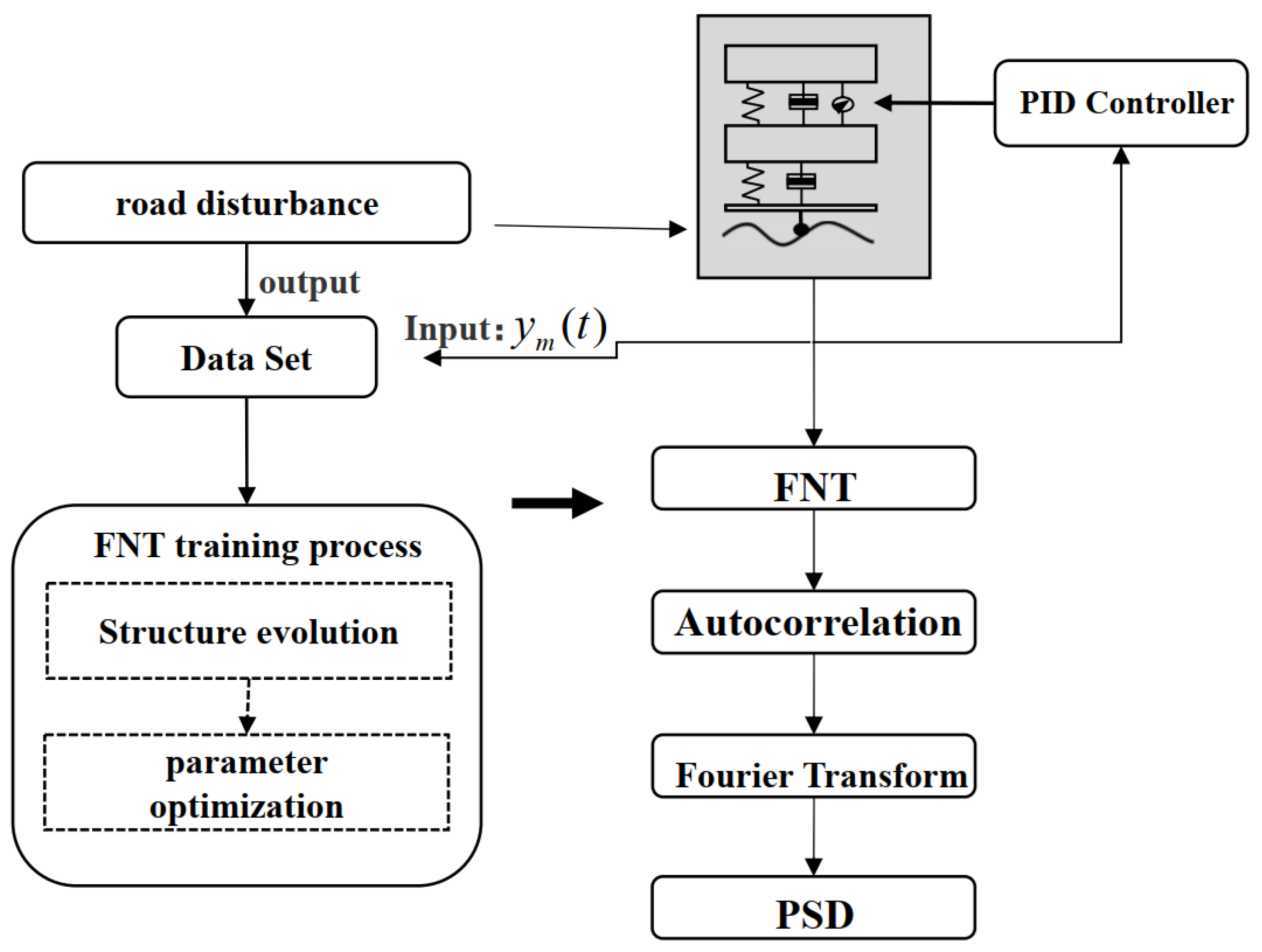
The continuous excitation of the road is the main source of body vibration. The road condition information provided by road detection techniques can provide accurate feedforward information for the design of adaptive control strategies for suspension systems. For semi-active suspension systems under the effect of uncertain parameters, a FNT-based algorithm for fitting the power spectral density of the road is proposed in this section, and the architecture is shown in Figure 3.

Firstly, the spring load speed, suspension deflection, spring mass and vehicle speed of the semi-active suspension are used as inputs, and the road vertical displacement perturbation information is used as an output to build the data set for training the FNT. The training process mainly consists of the structure evolution and the parameters optimization. Then the sensor collects the output $y_m$, vehicle speed and sprung mass of the suspension system in real time and fits the road vertical displacement by trained FNT. Finally, to extract further road features and eliminate noise effects, the time domain signal of the road vertical displacement perturbation is converted to road power spectral density values using the Fourier transform of the autocorrelation function.

3.1. FNT-Based Estimation of Road Vertical Displacement in Time Domain

In this study, FNT is employed to estimate the road vertical displacement. FNT is a neural network with a variable network structure, which is trained to simplify the structure and cut out unnecessary branches so that the network has as simple a structure as possible with high accuracy. A structural diagram of the flexible neural tree is shown in Figure 4, which is described as

$$S=F\cup T=\{{+}_1,{+}_2,...,{+}_N\}\cup \{x_1,...,x_n\},$$

(11)

where $+N$ is a non-leaf node with N child nodes and $x_n$ is a leaf node. The evolutive FNT process consists of two main parts: structural evaluation and parameter optimization. Firstly, random instructions are selected to create the neural tree. In the creation process of the neural tree, if ${+}_i$ is selected, i random connection weights $w_i$ and excitation random numbers ai and bi are generated, and the excitation of neuron $+i$ is given by

$$ne{t}_i=\sum _{j=1}^i{w}_j\ast x_j,$$

(12)

where $x_j$ is the input of node ${+}_i$, and the output of node ${+}_i$ is described as

$$ou{t}_i=e^{-{\left(\frac{ne{t}_i-a_i}{b_i}\right)}^2},$$

(13)

Before starting to optimize the tree structure, a population of tree structures needs to be generated. Then the genetic programming (GP) algorithm is used to evolve the structure of the FNT. GP is a learning algorithm inspired by biological evolution. It imitates random mutation and reproduction in biological evolution and selects the most suitable individuals to produce offspring through the fitness algorithm, which shown in Algorithm 1. Since this is a heuristic algorithm, we repeated it 50 times and used the best of them. Specific parameter values are shown in

Table 1. GP parameter values.

Parameter	Population Size	Max Generation	Max Tree Depth	Cross Rate	Mutation Rate
Value	40	40	3	0.8	0.2

.

Algorithm 1: The genetic programming (GP).

1.  Initialize population; 2.  fort = 1: maximum generation 3.        for i = 1: population size 4.           Get fitness evaluation $fi{t}_i$ for the i-th individual; 5.           if $fi{t}_i<fitnes{s}_{threshold}$ then probabilistically selected based on fitness; 6.           Generates the next generation through crossover and reproduction; 7.           Create a new population; 8.           Individuals are randomly selected for mutations; 9.           else Return the individual with the highest fitness; 10.       end 11.    end 12. end

After a better tree structure is determined, the particle swarm optimization (PSO) is used to optimize the parameters. The PSO algorithm is a kind of evolutionary algorithm. It starts from the random solution, finds the optimal solution through iteration, and evaluates the quality of the solution through fitness. It is easy to implement, with high precision, fast convergence, and good performance in solving practical problems. The pseudocode of PSO is shown in Algorithm 2. The PSO algorithm designs a massless particle that has only two properties: speed and position. Each particle represents a potential solution to the task within the search space. In the D-dimensional space, the position vector and velocity vector of the i-th particle can be expressed as $x_i=(x_{i1},x_{i2},\dots ,x_{iD})$ and $v_i=(v_{i1},v_{i2},\dots ,v_{iD})$, respectively. All particles in a swarm adjust their speed and position based on the current individual extremum they find and the current global optimal solution shared by the whole swarm. The velocity and position of the i-th particle are updated as follows:

$$\begin{array}{c}{v}_i(t+1)=w{v}_i\left(t\right)+c_1{r}_1(p_i-x_i\left(t\right))+c_2{r}_2(p_g-x_i\left(t\right)),\hfill \\ x_i(t+1)=x_i\left(t\right)+v_i(t+1),\hfill \end{array}$$

(14)

where w is the inertia weight, representing the influence of the previous velocity on the new one; $c_1$ and $c_2$ are learning factors, representing the update speed; $p_i$ represents the best previous position of the i-th individual, and $p_g$ denotes the best previous position of all particles in the current generation; $r_1$ and $r_2$ represent random values in the range $[0,1]$, respectively. Finally, we repeated the PSO algorithm 50 times and used the best one. Specific parameter values are shown in

Table 2. PSO parameter values.

Parameter	Population Size	Max Generation	w	${\mathit{c}}_1$	${\mathit{c}}_2$
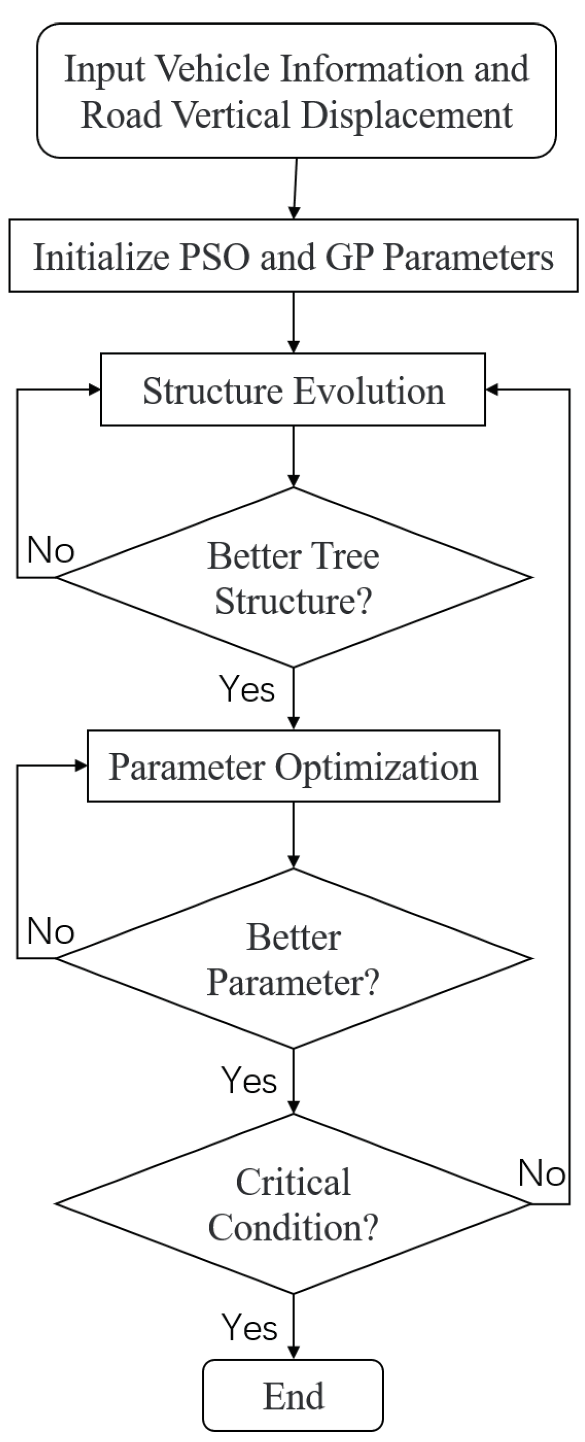
Value	20	200	0.73	1.49	1.49

. The road vertical displacement estimate algorithm, which is showed in Figure 5, can be described as following Algorithm 3.

Algorithm 2: Particle swarm optimization (PSO).

1.  Initialize population 2.  fort = 1: maximum generation 3.     for i = 1: population size 4.        if $f\left(x_{i,d}\left(t\right)\right)<f\left(p_i\left(t\right)\right)$ then $(p_i\left(t\right)=x_{i,d}\left(t\right)$ 5.           $f(p_g\left(t\right)=min(f\left(p_i\left(t\right)\right)$ 6.        end 7.        for d = 1: dimension 8.           $v_i(t+1)=w{v}_i\left(t\right)+c_1{r}_1(p_i-x_i\left(t\right))+c_2{r}_2(p_g-x_i\left(t\right))$ 9.           $x_i(t+1)=x_i\left(t\right)+v_i(t+1)$ 10.          if $(v_{i,d}(t+1)>v_{max}$ then $(v_{i,d}(t+1)=v_{max}$ 11.          else if $(v_{i,d}(t+1)<v_{max}$ then $(v_{i,d}(t+1)=v_{min}$ 12.          end 13.          if $(x_{i,d}(t+1)>v_{max}$ then $(x_{i,d}(t+1)=x_{max}$ 14.          else if $(x_{i,d}(t+1)<v_{max}$ then $(x_{i,d}(t+1)=x_{min}$ 15.          end 16.       end 17.    end 18. end

Algorithm 3: Road vertical displacement estimate algorithm based on FNT.

Input:    Sprung speed, ${\dot{z}}_s$; Suspension deflection, l$z_s-z_u$; Speed of vehicle, v; Sprung mass, $m_s$;     1: Initializing the parameters of PSO and GP; 2: Optimize the structure: If find the most suitable neural tree or reach the evolutionary algebra, then skip to step 3, else return to step 1; 3: Parameter optimization: PSO is used to optimize variable parameters; 4: If the number of iterations reaches the maximum or no better parameter is found, then skip to step 5, else return to step 3; 5: If the result reaches the preset condition or the number of times reaches the set value, then output the road Vertical disturbance d, else return to step 1. Output:    road vertical disturbance, d;

3.2. Road Power Spectral Density Fitting

Although the road vertical displacement signal can describe the time–domain characteristics of the road, the suspended time–domain signal is susceptible to the effects of pothole impact and noise, with large errors on the fitting effect. To minimize these disturbances and extract accurate road features and the frequency domain features of the road, the PSD is selected to describe the unevenness of the road. The signal power spectrum, which describes the signal power per unit frequency band, is a characteristic of road disturbance. The effect of low-frequency shock signals and high-frequency noise can be reduced by screening the power density in a certain frequency range. The correlated power spectrum estimation method adds a second truncated window to the autocorrelation function, which results in a smoother power spectrum and excellent noise resistance. The autocorrelation method is used in this subsection to convert the vertical displacement $d\left(k\right)$ of the road into a power spectral density value.

According to the Wiener–Sinchin theorem, the power spectral density of a signal is the Fourier transform of the autocorrelation function of the signal, so a segment of the road vertical displacement signal is first taken for the autocorrelation function analysis, and then the power spectral density of the segment is obtained by Fourier transform

$$\widehat{r}\left(m\right)=\frac{1}{N}\sum _{k=0}^{N-1-\left|m\right|}d\left(k\right)d(k+m),$$

(15)

where $d\left(k\right)$ is the vertical displacement of the road fitted by FNT, k is the serial number of the signal, N is the window size of the frequency conversion, and m is the translation distance. The Fourier transform of the autocorrelation function is sought to obtain the power spectral density

$$\widehat{S}\left(w\right)=\sum _{m=0}^M\widehat{r}\left(m\right)e^{-jwm},$$

(16)

where M is the upper limit of the frequency and the resulting $\widehat{S}\left(w\right)$ is an estimate of the road power spectral density for the window.

4. Adaptive Fuzzy PID Controller

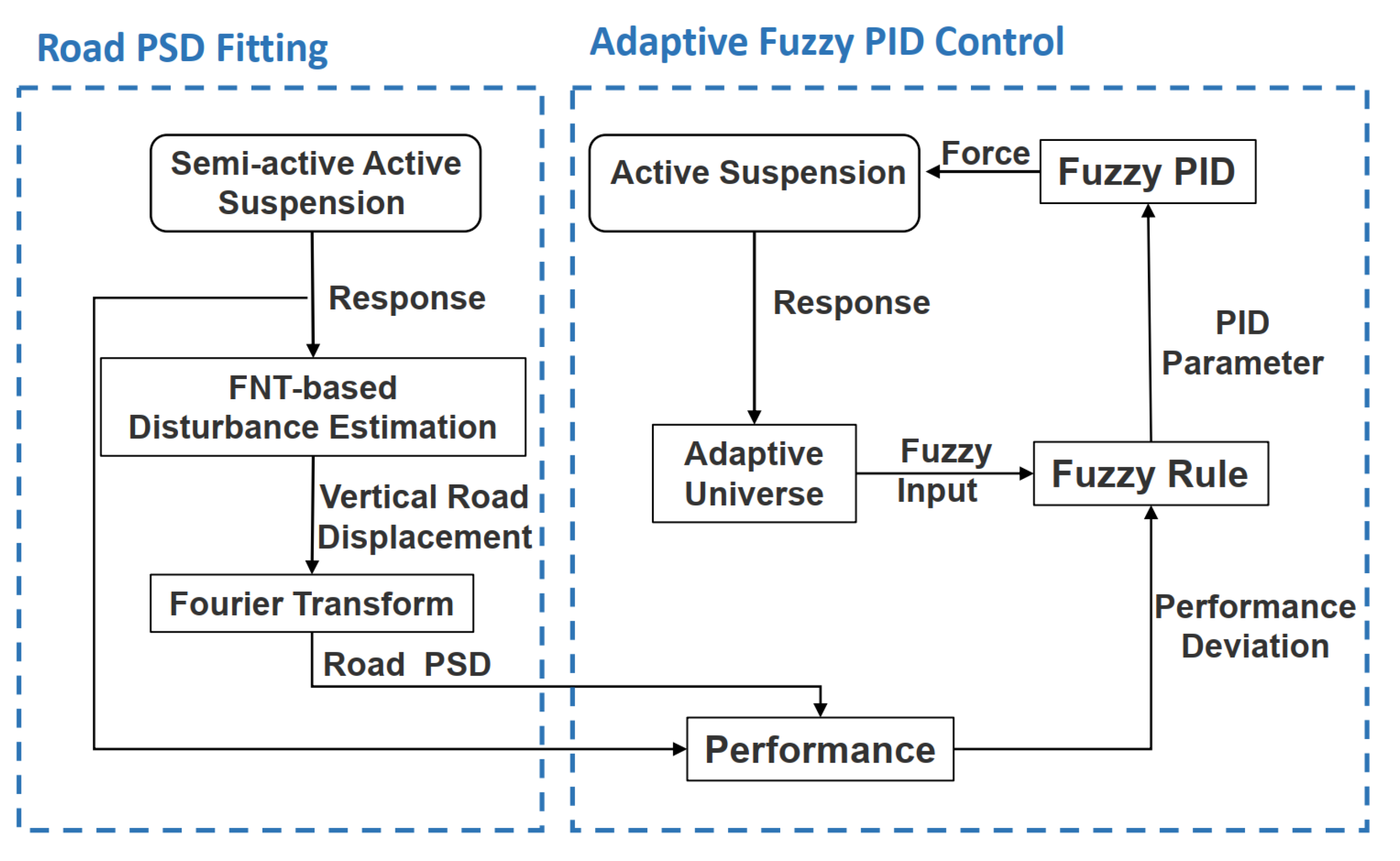
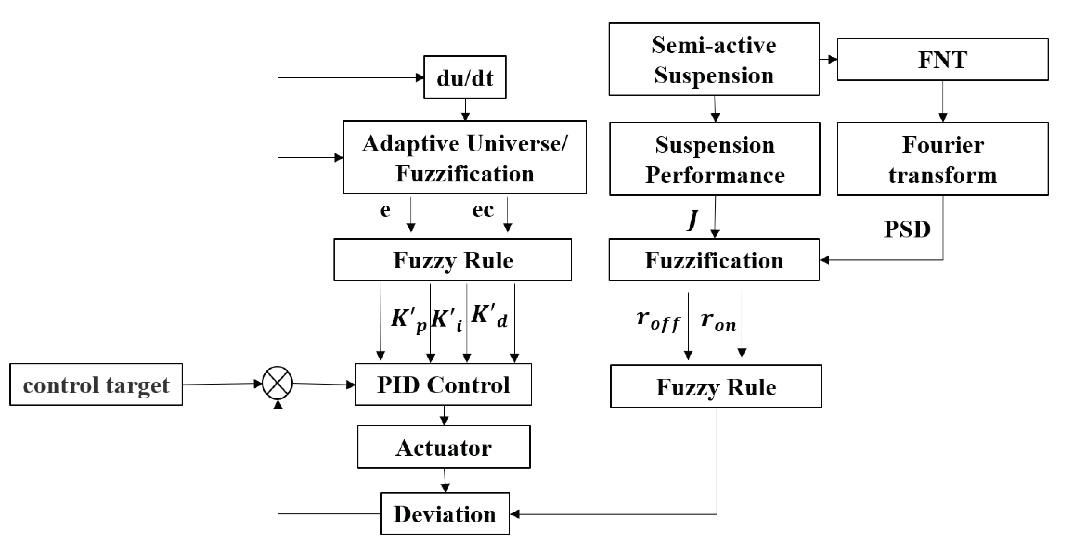
The adaptive fuzzy PID controller has two main parts: the online fuzzy evaluation of road conditions and the adaptive fuzzy PID control strategy. Its controller principle is shown in Figure 6.

Online fuzzy evaluation: Based on the dynamic information of the semi-active suspension received from the front half of the vehicle, the online performance prediction of the suspension system and the road PSD mean values obtained by FNT and Fourier transformation are fuzzed, and the road conditions are evaluated online fuzzy.

Adaptive fuzzy PID control strategy: Based on the fuzzy evaluation of road conditions, the fuzzy PID controller adaptively adjusts the control performance weighting for vehicle driving safety and comfort. The deviation of the performance indicators and their change rates are fuzzified in the basic domain of adaptive adjustment.

Fuzzy rules of fuzzy PID are designed based on the obtained fuzzy information to realize the real-time adjustment of the PID parameters $kp$, $ki$, and $kd$ so that the suspension system adaptively balances the weight of safety, comfort and suspension wear in the control according to the feedforward and feedback information to meet the control requirements of the suspension on different roads.

4.1. Real-Time Suspension Performance Fuzzy Evaluation Strategy

By combining the road power spectrum estimation with the real-time suspension performance, this subsection proposes an online fuzzy evaluation strategy for the road to reduce the time delay caused by a large sliding window and provides real-time road condition information for the control strategy.

First, the road PSD estimates are mapped from the basic definition domain to the fuzzy definition domain by introducing a quantization factor $r_{off}$, which describes the offline road conditions. Specifically, the energy signal in 10–80 Hz range is selected in the power spectrum by using the logarithm of the average power to quantify the road conditions. Meanwhile, $r_{off}$ is described as

$$r_{off}=\frac{1}{S}\sum _{w=10}^{80}lg\widehat{S}\left(w\right)$$

(17)

where S is the number of frequencies.

By using the obtained $r_{off}$ to describe the road condition information, the following membership functions are introduced, which includes “good road condition $S_{off}^1\left(r_{off}\right)$” and “poor road condition $S_{off}^2\left(r_{off}\right)$”, denoted as

$$S_{off}^1\left(r_{off}\right)=\frac{R_{off}^H-r_{off}}{R_{off}^H-R_{off}^L},S_{off}^2\left(r_{off}\right)=\frac{r_{off}-R_{off}^L}{R_{off}^H-R_{off}^L}$$

(18)

where $R_{o}f{f}^H$ and $R_{o}f{f}^L$ are the maximum and minimum values of the road power spectral density, respectively.

Real-time suspension dynamic performance $J\left(k\right)$ is introduced into the online road condition assessment in order to better capture changes in the road conditions and reduce the time delay caused by the estimation of the road power spectrum. The real-time suspension dynamic performance $J\left(k\right)$ is defined as

$$J\left(k\right)=max\left(\left|\left|y_{m1}\left(k\right)-y_{m1}\left(k-1\right)\right|-\left|y_{m1}(k-1)-y_{m1}\left(k-2\right)\right|\right|\right),k\in [k_0-T_j,k_0],$$

(19)

where $k_0$ is the current ordinal number and $T_j$ is the performance window size, which could be as small as possible to meet the real-time requirements. Based on the performance metric $J\left(k\right)$ measured in real time, the following membership functions are introduced, which includes “good performance $S_{on}^1\left(J\left(k\right)\right)$” and “poor performance $S_{on}^2\left(J\left(k\right)\right)$” and is described as

$$S_{on}^1\left(J\left(k\right)\right)=\frac{{log}_{2}J\left(k\right)-{log}_2{J}_{min}}{{log}_2{J}_{max}-{log}_2{J}_{min}},S_{on}^2\left(J\left(k\right)\right)=\frac{{log}_2{J}_{max}-{log}_{2}J\left(k\right)}{{log}_2{J}_{max}-{log}_2{J}_{min}}$$

(20)

where $J_{\min }$ and $J_{\max }$ are the maximum and minimum values of the suspension performance $J\left(k\right)$. Based on the above membership function, the following adaptive adjustment model for control performance weights is described as

$$\begin{array}{c}Rulei:IF{r}_{off}\left(k\right)is{S}_{off}^l\left(r_{off}\left(k\right)\right)andJ\left(k\right)is{S}_{on}^r\left(J\left(k\right)\right)\hfill \\ THEN\hfill \\ e_i\left(k\right)={\alpha }_i\times y_c\left(k\right)={\left[\begin{array}{c}{\alpha }_{i1}\hfill \\ {\alpha }_{i2}\hfill \\ {\alpha }_{i3}\hfill \end{array}\right]}^T\left[\begin{array}{c}\begin{array}{c}{\ddot{z}}_s\left(k\right)\\ z_s\left(k\right)-z_u\left(k\right)\end{array}\hfill \\ z_u\left(k\right)-z_r\left(k\right)\hfill \end{array}\right]\hfill \end{array}$$

where $l=1,2$, and $r=1,2$.

By using the fuzzy blending approach, the overall performance evaluation value $e\left(k\right)$ of the system can be described as

$$e\left(k\right)=\sum _{i=1}^4{\mu }_i(r_{off}\left(k\right),r_{on}\left(k\right))e_i\left(k\right)$$

(21)

where

$$\begin{array}{c}{\mu }_1(r_{off}\left(k\right),J\left(k\right))=S_{off}^1\left(r_{off}\left(k\right)\right)\times S_{on}^1\left(J\left(k\right)\right),\hfill \\ {\mu }_2(r_{off}\left(k\right),J\left(k\right))=S_{off}^1\left(r_{off}\left(k\right)\right)\times S_{on}^2\left(J\left(k\right)\right),\hfill \\ {\mu }_3(r_{off}\left(k\right),J\left(k\right))=S_{off}^2\left(r_{off}\left(k\right)\right)\times S_{on}^1\left(J\left(k\right)\right),\hfill \\ {\mu }_4(r_{off}\left(k\right),J\left(k\right))=S_{off}^2\left(r_{off}\left(k\right)\right)\times S_{on}^2\left(J\left(k\right)\right).\hfill \end{array}$$

4.2. Adaptive Fuzzy PID Controller

According to the adaptive fuzzy PID controller control schematic, the following adjustment rules are obtained for the two-input, three-output fuzzy controller.

$$\left\{\begin{array}{c}{K}_p^{{}^{\prime }}\left(k\right)=K_{p0}+\Delta K_p\left(k\right)\times q_p\hfill \\ K_i^{{}^{\prime }}\left(k\right)=K_{i0}+\Delta K_i\left(k\right)\times q_i\hfill \\ K_d^{{}^{\prime }}\left(k\right)=K_{d0}+\Delta K_d\left(k\right)\times q_d\hfill \end{array}\right.,$$

(22)

where $k_{p0}$, $k_{i0}$, and $k_{d0}$ represent the initial scale, integration and differentiation coefficients of the PID controller; $K_p{\left(k\right)}^{{}^{\prime }}$, $K_i{\left(k\right)}^{{}^{\prime }}$, and $K_d{\left(k\right)}^{{}^{\prime }}$ represent the adjusted parameters; $\Delta K_p\left(k\right)$, $\Delta K_i\left(k\right)$, and $\Delta K_d\left(k\right)$ are the PID control quantities output from the fuzzy controller; and $q_p$, $q_i$, and $q_d$ are the amplification scale factors.

From the basic principle of PID control, it can be seen that the adjustment of the PID parameters in real time should follow the principles under the action of different input quantities and error variations:

(1)

When E and $EC$ are in the same direction, the actual value of the system will deviate further from the set value. At this time, the controller needs to quickly reduce the error so as to expedite the response of the system, so the control amount needs to be increased and reversed.

(2)

When E and $EC$ are reversed, the actual value of the controlled system will change in the direction of stability, in which case the controller should reduce the control amount.

(3)

When E is large, overshoot can be suppressed in advance by differential action in order to overcome inertia-induced overshoot.

Based on the above principles, a fuzzy rule obtained by simple reasoning is shown in

Table 3. Fuzzy rule table of $K_p$, $K_i$, and $K_d$.

$\mathit{EC}$	E
	PB	NB	NM	NS	ZO	PS	PM
NB	PB/NB/PB	PB/NB/PB	PB/NB/PB	PB/NB /ZO	PM/NM/PB	PS/NS/PM	ZO/ZO/NS
NM	PB/NB/PB	PB/NB/PB	PM/NM/PM	PM/NM/ZO	PS/NS/PB	ZO/ZO/PS	ZO/ZO/NM
NS	PB/NB/PB	PM/NM/PM	PS/NS/PM	PS/NS/ZO	ZO/ZO/PM	ZO/ZO/ZO	NS/PS/NB
M	PM/NM/NB	PS/NS/NM	PS/NS/NS	ZO/ZO/ZO	NS/PS/NS	NS/PS/NS	NM/PM/NB
PS	PS/NS/NB	ZO/ZO/ZO	ZO/ZO/PM	NS/PS/ZO	NM/PM/PM	NM/PM/NM	NB/PB/PB
PM	ZO/ZO/NM	ZO/ZO/PS	NS/PS/PB	NM/PM/ZO	NM/PM/PM	NB/PB/PB	NB/PB/PB
PB	ZO/ZO/NS	NS/PS/PM	NM/PM/PB	NB/PB/ZO	NB/PB/PB	NB/PB/PB	NB/PB/PB

. The fuzzy rules refer to the literature [21], in which the fuzzy PID control is also the control of the object in the high-speed state. The control rules combine the previous PID regulation experience and improve the overshoot caused by inertia, so as to speed up the regulation and reduce the overshoot.

Based on the above rules, this section designs a fuzzy controller with E and $EC$ as fuzzy inputs and $\Delta K_p\left(k\right)$, $\Delta K_i\left(k\right)$, and $\Delta K_d\left(k\right)$ as outputs, where E and $EC$ are described by seven fuzzy subsets, and also by seven fuzzy subsets for $\Delta K_p\left(k\right)$, $\Delta K_i\left(k\right)$, and $\Delta K_d\left(k\right)$, whose definition domains are all set to $[-1,1]$ and defined as

$$\left\{\begin{array}{c}E,EC=\{NB,NM,NS,ZO,PS,PM,PB\},E,EC\in [-1,1]\hfill \\ \Delta K_p,\Delta K_i,\Delta K_d=\{NB,NM,NS,ZO,PS,PM,PB\},\Delta K_p,\Delta K_i,\Delta K_d\in [-1,1]\hfill \end{array}\right.,$$

(23)

where NB, NM, NS, ZO, PS, PM and PB are used to represent the seven levels from positive to negative, as shown in the Equation (27).

To obtain the input fuzzy quantities E and $EC$, the paper uses $e\left(k\right)$ with its variation $e\left(k\right)-e(k-1)$ as the input variables for fuzzy control and defines their corresponding fundamental domains as $[-x_{em}\left(k\right),x_{em}\left(k\right)]$ and $[-x_{ecm}\left(k\right),x_{ecm}\left(k\right)]$. Since the response range of the vehicle suspension varies considerably when the vehicle is driven on different roads, the effective values of $x_{em}\left(k\right)$ and $x_{em}\left(k\right)$ change as the road changes, and the size of the fundamental domain needs to be adaptively adjusted in real time as follows.

$$\left\{\begin{array}{c}{x}_{em}\left(k\right)=max\left(e\left(k\right)\right),k\in [k-T_f,k]\hfill \\ x_{ecm}\left(k\right)=max[e\left(k\right)-e(k-1)],k\in [k-T_f,k]\hfill \end{array}\right.$$

(24)

where $T_f$ is the adaptive adjustment window.

In order to achieve fuzzy control, it is necessary to adjust the input variables from the fundamental domain to the definition domain.

$$\left\{\begin{array}{c}E=p_{e}e\left(k\right)\hfill \\ EC=p_{ec}[e\left(k\right)-e(k-1)]\hfill \end{array}\right.$$

(25)

where $p_e=1/x_{em}$ and $p_{ec}=1/x_{ecm}$. To map the specific values of the fuzzy output to the fuzzy sets, a quantization function needs to be introduced. In this paper, a linear approach to quantization is used

$$f\left(x\right)=\left\{\begin{array}{c}0x\le -1\hfill \\ \frac{x+1}{2}-1<x\hfill \\ 1x\ge -1\hfill \end{array}\right.<1$$

(26)

Next comes the determination of the membership degree of E and $EC$ on the fuzzy subsets. In this experiment, a triangular membership function is used, and Figure 7 shows the image of the membership function with the following equation:

$$g(f\left(x\right),a,b,c)=max(0,min(\frac{f\left(x\right)-a}{b-a},\frac{c-f\left(x\right)}{c-b}))$$

(27)

where a, b and c are the parameters of the triangular membership function and x is the fuzzy input.

To simplify the calculation process, the output $\Delta K_p\left(k\right)$, $\Delta K_i\left(k\right)$, and $\Delta K_d\left(k\right)$ also use a triangular membership function, as shown in Figure 7, and are defuzzified using the center of gravity method, which is described as

$$w_0=\frac{{\displaystyle \sum _{i=0}^n}g(w_i,a_i,b_i,c_i)\ast w_i}{{\displaystyle \sum _{i=0}^n}g(w_i,a_i,b_i,c_i)},$$

(28)

where $w_0$ is the exact value of the fuzzy controller output after defuzzification; $w_i$ is the value in the domain of the fuzzy control quantity; $g(w_i,a_i,b_i,c_i)$ is the membership degree of $w_i$ in the membership function with parameters $a_i,b_i,c_i$.

Overall, this section obtains the PID parameter adjustments $\Delta K_p\left(k\right)$, $\Delta K_i\left(k\right)$, $\Delta K_d\left(k\right)$ by adaptive fuzzy rules using $e\left(k\right)$ and $e\left(k\right)-e(k-1)$ as fuzzy inputs, and uses the adjusted parameters $K_p{\left(k\right)}^{{}^{\prime }}$, $K_i{\left(k\right)}^{{}^{\prime }}$, and $K_d{\left(k\right)}^{{}^{\prime }}$. Thus the PID controller $u\left(k\right)$ is obtained as

$$u\left(k\right)=K_p^{{}^{\prime }}\left(k\right)[e\left(k\right)-e(k-1)]+K_i^{{}^{\prime }}\left(k\right)e\left(k\right)+K_d^{{}^{\prime }}\left(k\right)[e\left(k\right)-2e(k-1)+e(k-2)]+u(k-1).$$

(29)

It should be noted that the controller uses FNT with a simple structure to recognize the vertical displacement of the road surface, and uses a small sampling window to extract the PSD of the road surface, which reduces the computational complexity and improves the computational speed. In order to improve the matching speed of the fuzzy rules, the four fuzzy inputs are slitted into two fuzzy systems, which reduces the number of fuzzy rules and improves the operation speed.

5. Simulation and Analysis

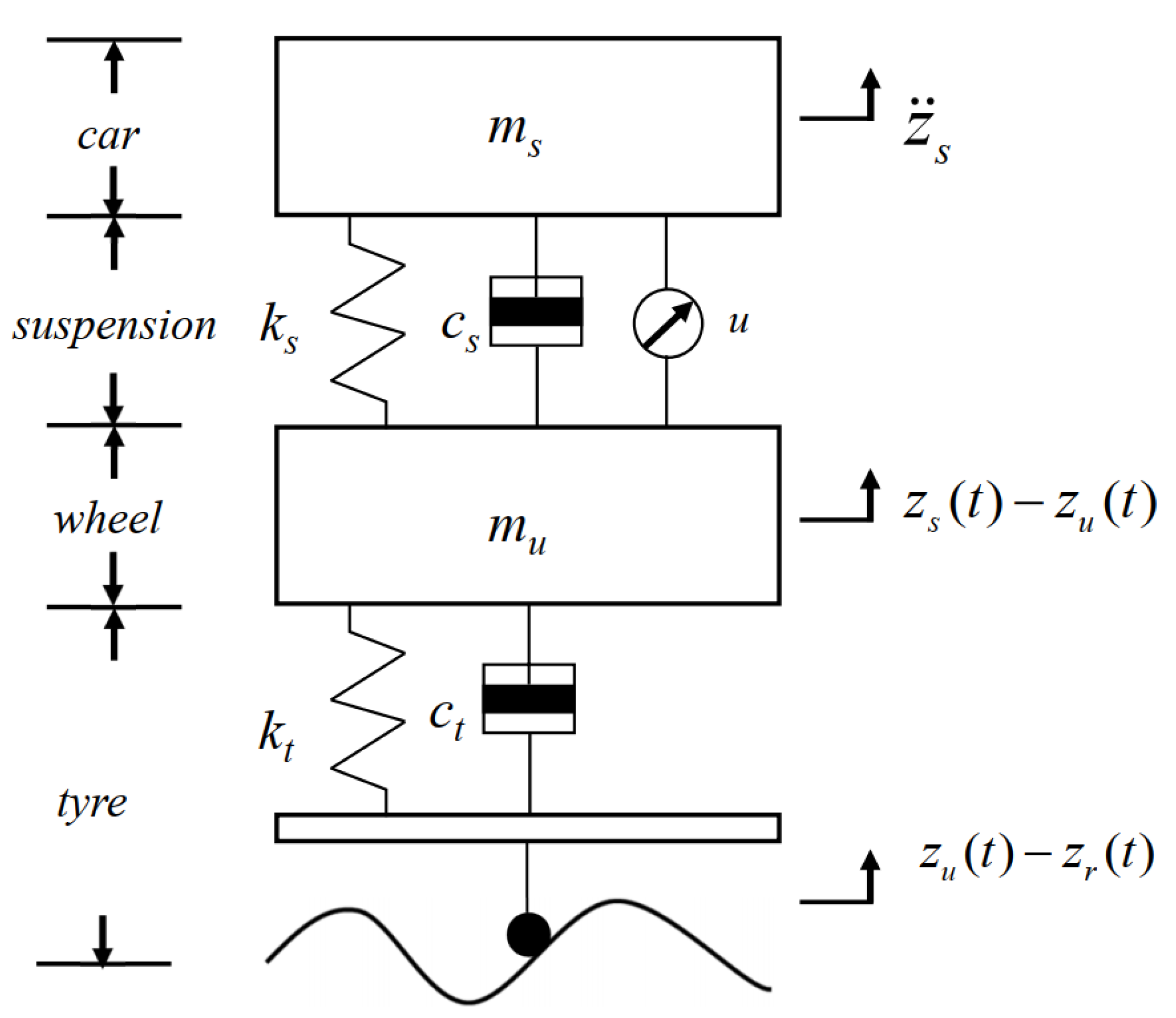
In this paper, a classical quarter suspension system is introduced to verify the performance of the fuzzy PID control strategy in the case of different level roads; the suspension system parameters are shown in

Table 4. Parameters for a 1/4 vehicle model.

Parameter	Symbol	Value	Unit
Sprung mass	$m_s$	972.2	kg
Unsprung mass	$m_t$	113.6	kg
Damping coefficient of suspension	$c_s$	1095	Ns/m
Damping coefficient of pneumatic tire	$c_t$	14.6	Ns/m
Spring stiffness	$k_s$	42,719.6	N/m
Tire stiffness	$k_t$	10,115	N/m

.

To verify the effectiveness of the proposed fuzzy PID control strategy for damping on different road conditions, a simulated test road is constructed in MATLAB/SIMULINK. The simulated road consists of 10 different levels of road under ISO8608 for a total of 2 km, which fully considers a variety of road changes. The road surface is continuously disturbed, and multiple road surfaces and road switching are considered. The vehicle is driven at a constant speed of 20 m/s, and the road level changes every 10 seconds.

In order to analyze the quality of damping, we focus on the following performance indicators:

(1)

The adjustment time $T_{p-n}=t_{sp}-t_{en}$ for the suspension system from good road to poor road; $t_{sp}$ is the time when the suspension system starts to move to the small oscillation range, and $t_{en}$ is the time when the large oscillation range resumes.

(2)

The adjustment time $T_{n-p}=t_{sn}-t_{ep}$ for the suspension system from poor road to good road; $t_{sn}$ is the time when the suspension system starts to move out of the large oscillation range, and $t_{ep}$ is the time to regain the small oscillation range.

(3)

RMS of the sprung speed of the suspension during the whole distance.

$$s_{rms}=\sqrt{\frac{1}{N}\sum _{t=0}^{t_n}{y}_{c1}{\left(k\right)}^2}$$

(30)

(4)

RMS of suspension dynamic deflection during the whole distance.

$$x_{rms}=\sqrt{\frac{1}{N}\sum _{t=0}^{t_n}{y}_{c2}{\left(k\right)}^2}$$

(31)

(5)

RMS of dynamic tire deflection on roads from G to H.

$$z_{rms-n}=\sqrt{\frac{1}{M}\sum y_{c3}{\left(k_N\right)}^2}$$

(32)

where $K_N$ is the ordinal number on roads from G to H.

5.1. Analysis of Road Fitting

This subsection verifies the effectiveness of the proposed FNT-based road fitting algorithm. The data set used for this training road fitter is obtained under MATLAB/SIMULINK. The road contains 20,000 pieces of data of A–H grade 8 highway under ISO8606 standard [20], of which 80% is the training sets and 20% is the verification sets. The sprung mass $m_s$ varies from 600 to 1000 kg, the vehicle speed v varies from 5 to 25 m/s, and the sensor uses 200 Hz as a sampling rate.

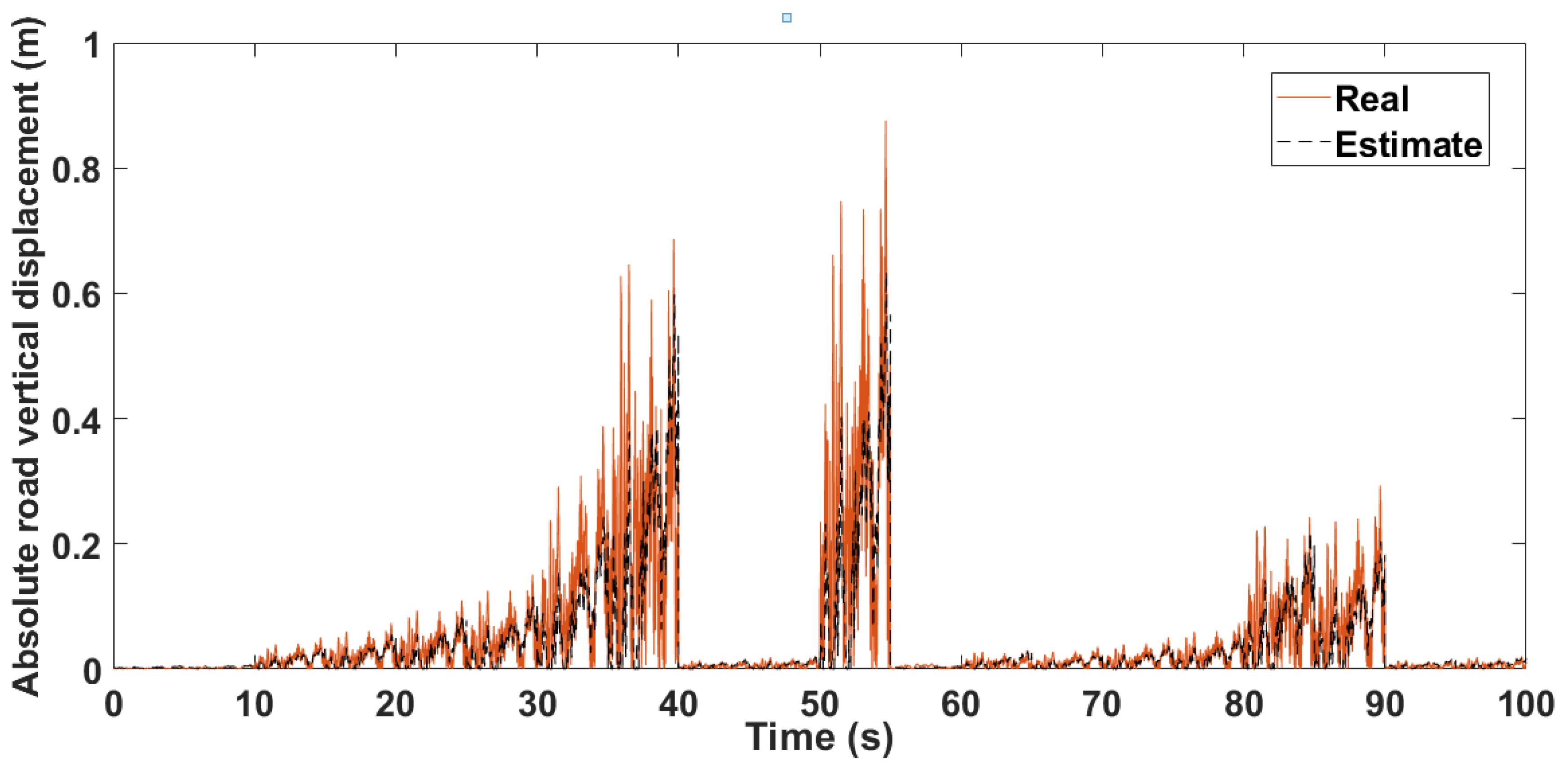
By using the FNT-based road estimation algorithm in the time domain, the estimated road vertical displacement is compared with the real road vertical displacement as shown in Figure 8. The RMS of the test error is 0.0592, which is a good fit.

After obtaining the road vertical displacement, the Fourier transform of autocorrelation is used to obtain the PSD. In order to verify the effect of the Fourier transform of autocorrelation, it is compared with the periodogram method in terms of noise resistance performance as shown in Figure 9. After a comparison of the time domain signal with the addition of random noise, it is found that the latter has better noise resistance and better smooth performance.

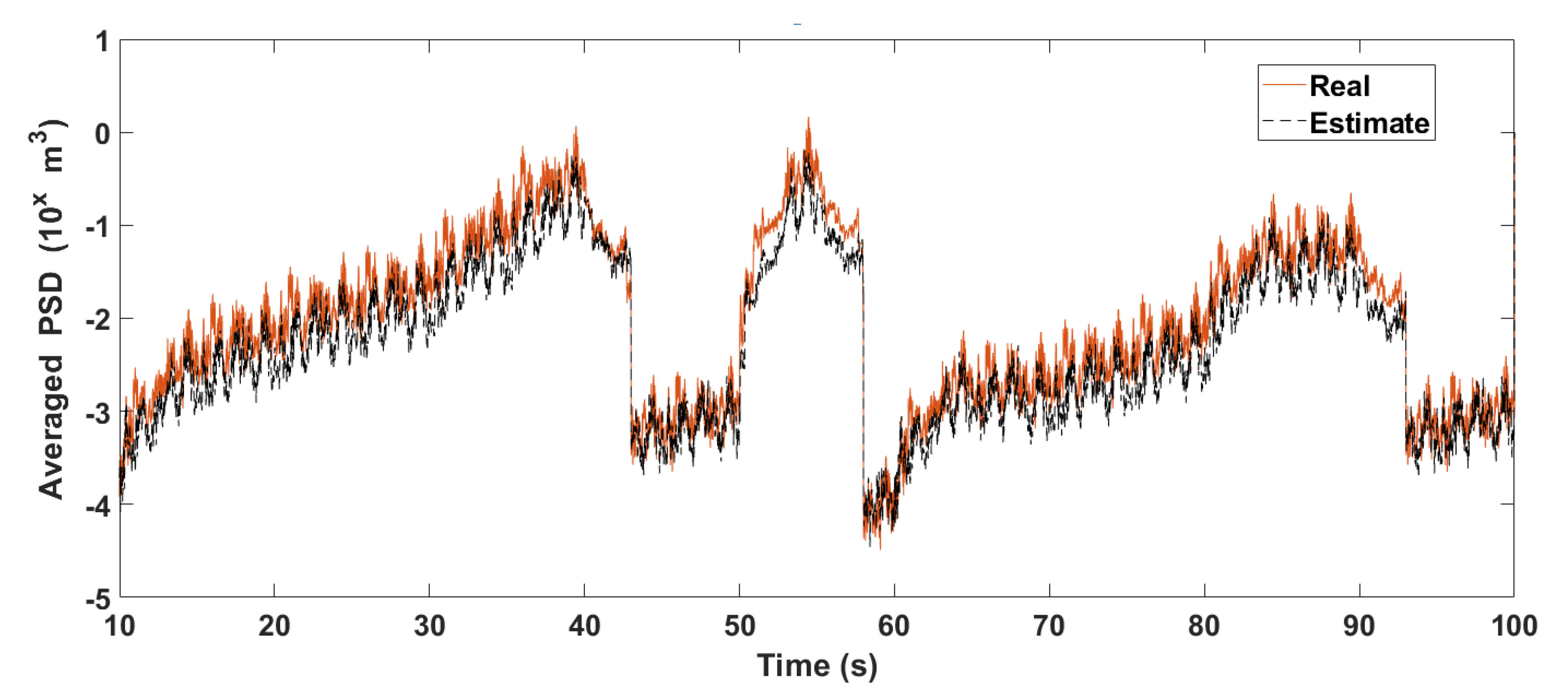
The error RMS of the effect of the added noise on the original power density spectrum is 0.1429 when the periodogram method is used, and 0.1429 when the correlated power spectrum estimation method is used, demonstrating the better noise resistance of the correlated power spectrum method. The Fourier transform of autocorrelation is used to transform the fitted road disturbance in the frequency domain, and the average road PSD $\widehat{s}\left(w\right)$ is obtained. The comparison between the real $\widehat{s}\left(w\right)$ and the fitted $\widehat{s}\left(w\right)$ is shown in Figure 10, with an error RMS of $0.3182$, which shows a good fit of the PSD.

5.2. Analysis of PID Control Effects

This subsection tests the control effectiveness of the proposed adaptive fuzzy PID control strategy.

The control performance of the suspension system is measured when the vehicle is driven on the simulated road. In order to highlight the adaptive control effect of this method when facing different road conditions, four special situations during the test are selected to demonstrate the control effect. The main parameter settings of the adaptive fuzzy PID controller are shown in

Table 5. Adaptive fuzzy PID controller setting parameters.

Parameter	${\mathit{K}}_{\mathit{p}0}$	${\mathit{K}}_{\mathit{i}0}$	${\mathit{K}}_{\mathit{d}0}$	${\mathit{q}}_{\mathit{p}}$	${\mathit{q}}_{\mathit{i}}$	${\mathit{q}}_{\mathit{d}}$
Value	3000	1000	300	1	0.1	0.1

.

In order to prove the effectiveness of the proposed controller, the following scenarios are considered.

Scenario 1: In 60 s, the vehicle moves from the H-level road to D-level road in order to test the rapid stability of the suspension system for road changes. The sprung speed is selected here as stable performance, as shown in Figure 11A. The specific performance indicators are shown in

Table 6. Performance of suspension in test.

	${\mathit{T}}_{\mathit{p}-\mathit{n}}$	${\mathit{T}}_{\mathit{n}-\mathit{p}}$	${\mathit{s}}_{\mathbf{rms}}$	${\mathit{z}}_{\mathbf{rms}-\mathit{n}}$	${\mathit{x}}_{\mathbf{rms}}$
passive control	3 s	7 s	1.5176	2.7021	0.2195
PID control	1.5 s	2.5 s	0.5127	0.6801	0.1171
Our method	0.7 s	1 s	0.0926	0.1517	0.1379

.

Scenario 2: In 50 s, the vehicle moves from the C-level road to H-level road. The sprung speed is shown in Figure 11B, and the specific performance indicators are shown in Table 6.

According to the above results, it can be observed that compared with the PID suspension and passive suspension, the fuzzy PID control method based on road surface estimation can stabilize the suspension faster and better when the road surface changes greatly because the method can carry out rapid estimate and correct control of the road so that the suspension is better adaptable to the changing road.

Scenario 3: In 30 s, the vehicle moves from the E-level road to G-level road in order to show the improvement in the safety. The tire deflection is selected here as the grip performance. The specific display is shown in Figure 11C, and the specific performance indicators are shown in Table 6.

According to the test results, our control method shows an adaptable performance in adjusting the weights when the road is poor, making the suspension performance more grippy and ensuring the safety of the vehicle when the road is poor.

Scenario 4: To test the effect of the control method on the wear and service life of the suspension system, we tested the suspension deflection while the vehicle is running, as shown in the Figure 11D for the first 30 s, with the specific performance indicators shown in Table 6.

The specific indicators of the simulation tests are shown in Table 6 from which it can be observed that, compared to the passive control and the PID control, our method displays a greater improvement in speed adjustment when the road changes, better performance in controlling the sprung speed with better comfort, and better tire grip when the road is poor, thus ensuring the safety of the vehicle. The suspension deflection is close to the effect of the PID control, verifying its lifetime performance.

In addition, in order to verify the effectiveness of our method, we compare it with the switched reluctance method (SR) [22] and observer-based multi-objective integrated (OMI) [23] method under the same random road environment. The comparison results are shown in

Table 7. Comparison with SR and OMI.

	${\dot{\mathit{s}}}_{\mathit{rms}}$	${\mathit{z}}_{\mathit{rms}}$	${\mathit{x}}_{\mathit{rms}}$
Our method	0.4293	0.0019	0.0163
SR method	0.2956	0.0011	0.0019
OMI method	0.5856	0.0026	0.0156

, where ${\dot{S}}_{RMS}$ represents the RMS of suspension acceleration. Although the control comfort and grip performance of our method are not as good as the SRM method, the performance is better than the OMI method. These two methods focus on vibration reduction control of road surface at the same level, while our method focuses on the rapid adjustment ability of suspension system when road switch, and our method has better adaptability in the face of complex and changeable road surfaces. It is worth mentioning that our method uses the PID controller combined with a sensor, which is more cost effective than other methods and easier to apply in a wide range.

6. Conclusions

It is well known that the PID controller is the most widely used controller in the industrial field, and has been applied to a variety of vehicle suspension controls. It has high application value to improve the PID controller to overcome its shortcomings.

In this paper, the road power spectrum analysis was combined with the online suspension real-time performance to obtain real-time fuzzy road information, which was used to adjust the control performance of fuzzy PID so as to develop a new road condition-based fuzzy PID control strategy. By using the road condition-based fuzzy PID controller proposed, the safety, comfort and stability of the vehicle can be attained under different road conditions. According to the numerical simulation results, the proposed control strategy can improve the performance of the vehicle significantly, compared with the passive control of the suspension and the PID control of the suspension, owning to its different priorities of control performance trade-offs for different road conditions.

This paper is under the assumption that the suspension system is an ideal model and ignores external interference factors, such as friction. The test road surface is also ideal without external interference. Meanwhile, this study could meet the requirements of special vehicles in complex and changeable road conditions for driving, especially in field roads to better guarantee driving safety. In the future work, the real suspension system could be used for experimental simulation based on the data obtained from real detection. Furthermore, the road recognition results should be integrated with other control strategies to reduce vehicle suspension deflection and service wear.