Abstract
This paper proposes a novel robust latent common subspace learning (RLCSL) method by integrating low-rank and sparse constraints into a joint learning framework. Specifically, we transform the data from source and target domains into a latent common subspace to perform the data reconstruction, i.e., the transformed source data is used to reconstruct the transformed target data. We impose joint low-rank and sparse constraints on the reconstruction coefficient matrix which can achieve following objectives: (1) the data from different domains can be interlaced by using the low-rank constraint; (2) the data from different domains but with the same label can be aligned together by using the sparse constraint. In this way, the new feature representation in the latent common subspace is discriminative and transferable. To learn a suitable classifier, we also integrate the classifier learning and feature representation learning into a unified objective and thus the high-level semantics label (data label) is fully used to guide the learning process of these two tasks. Experiments are conducted on diverse data sets for image, object, and document classifications, and encouraging experimental results show that the proposed method outperforms some state-of-the-arts methods.
1. Introduction
Collecting massive labeled data is an expensive and time-consuming process in realistic scenarios [1]. Meanwhile, visual classification models often are required to be well trained for accurate prediction by sufficient labeled data. In this case, there is an urgent need to use labeled and relevant data from various data sets for facilitating the training process [2]. However, in some complex applications, the data from different data sets have different distributions. Thus, the key point of the problem is how to recover the knowledge gained from existing or well-constructed data sets for a novel task. Transfer learning is such a technique that attempts to learn an appropriated model for target application by recovering the knowledge from the source domain [3,4] In other words, transfer learning attempts to transfer the knowledge from the source domain where the data are labeled to a different but related target domain for obtaining a better model [5,6].
A major problem in transfer learning is how to decrease the different probability distributions of data in source and target domains. Intuitively, finding a better data representation that not only reduces the discrepancy distributions among different domains as best as we can but also simultaneously preserves essential properties (such as local geometric properties and intrinsic discriminable structure of data) of different domains is a feasible solution [7] which makes the model trained from the labeled source domain use for target domain directly. Many conventional subspace learning methods aim to find a good data representation (low dimensional subspace) that can preserve some specific properties of original data and thus they can be used for transfer learning [8,9,10,11]. Transfer subspace learning methods use the idea of subspace learning to find an appropriate data representation, i.e., latent common subspace, for the data of source and target domains in which the different distributions of the source and target data are also reduced as much as possible [12,13,14]. Nonetheless, these proposed transfer subspace learning methods only focus on low-level features (visual features) of data from the source and target domains, which are independent of the subsequent tasks such as visual classification. Thus, the high-level semantic information (label information) is not fully exploited to guide classifier learning [15,16].
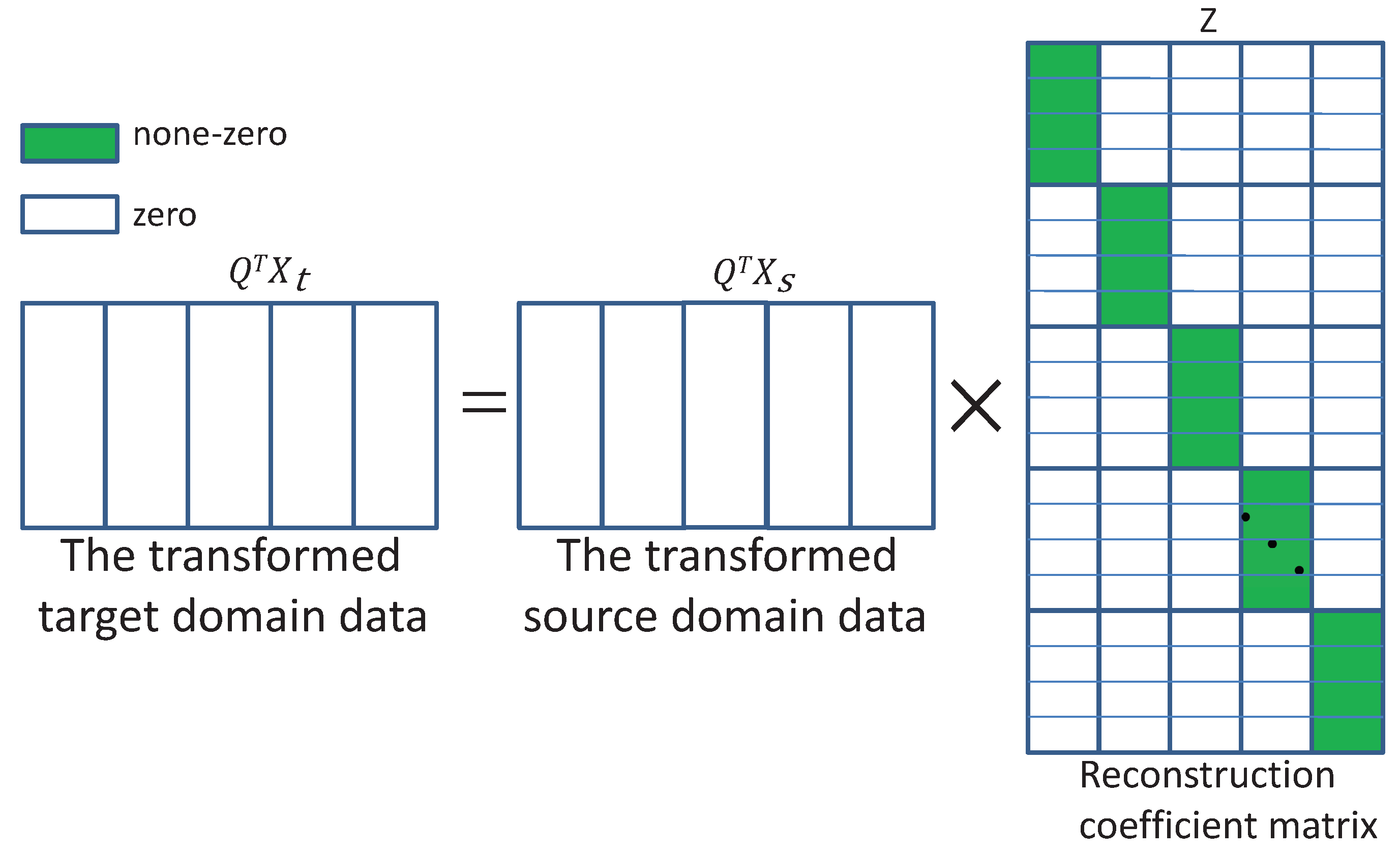
It is well known that in transfer learning a good feature representation should be transferable [2,3,5]. However, to learn a discriminative classifier, we need to learn a discriminative feature representation. Therefore, we assume that we can learn a discriminative and transferable feature representation from the original feature representation. To this end, this paper attempts to find an appropriate data feature representation for reducing the difference in probability distributions between different domains. Therefore, this paper proposes a novel transfer learning method called robust latent common subspace learning (RLCSL) by finding a proper data feature representation that can not only reduce the distribution discrepancy but also improve the discriminative ability of the new feature representation. In this way, the new feature representation is beneficial for the subsequent learning task, i.e., classifier learning. Previous transfer subspace learning methods merely focus on the transferable feature representation learning. However, the proposed method uses data reconstruction to find a latent common subspace where the data from source and target domains have similar probability distributions by using the low-rank constraint. Moreover, the data from different domains but with the same label can be aligned together by using the sparse constraint. Current locality reconstruction methods only work on the scenario that the data come from the same domain, i.e., the data have a similar distribution. For example, locally linear embedding (LLE) [17] and non-negative matrix factorization (NMF) [18] cannot guarantee a neighborhood-to-neighborhood reconstruction. To this end, the proposed method imposes low-rank and sparse constraints on the reconstruction coefficients which can make the reconstruction coefficient matrix obtain a block-wise structure as shown in Figure 1. Therefore, the neighborhood-to-neighborhood reconstruction can be obtained. Specifically, we introduce the low-rank and sparse constraints to constrain the reconstruction coefficient matrix to achieve this goal so that the reconstruction process can automatically select the neighbor data sharing the same label but from different domains to complete the reconstruction as much as possible [15,19]. To enhance the robustness of our algorithm, we also introduce a sparse matrix to simulate the noise for reducing the effect of noisy data during the data reconstruction. To learn a suitable classifier parameter, we integrate the classifier learning and feature representation learning into a unified optimization objective. The whole framework of our method is demonstrated in Figure 2. We apply the proposed RLCSL method to the task of transfer learning. Massive experiments are conducted on the image data, object data, and document data and encouraging experiment results show the outstanding performance of our method.
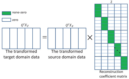
Figure 1.
The transformed target domain data is represented by the transformed source domain data and the reconstruction coefficient matrix has a block-wise structure.

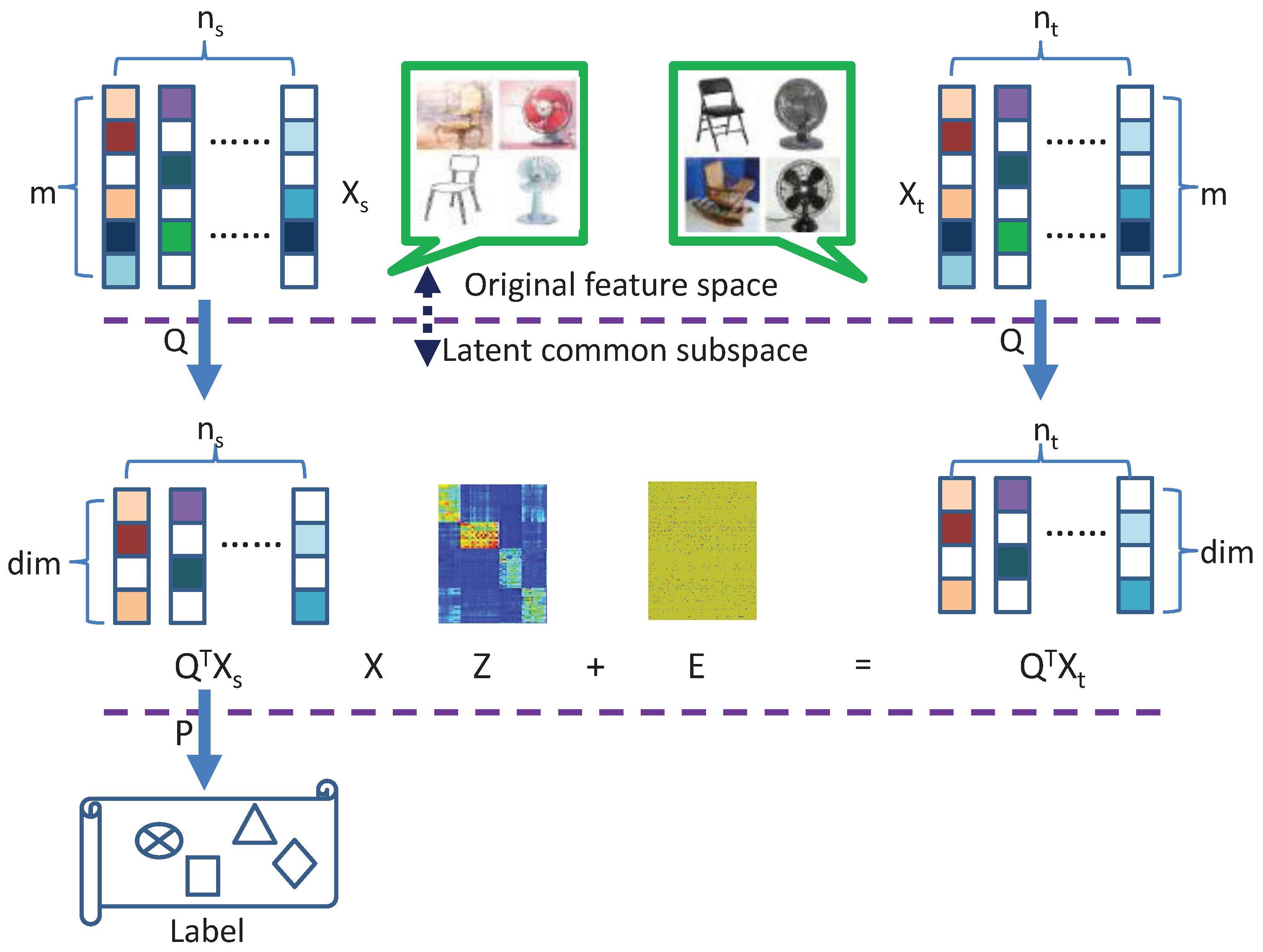
Figure 2.
Framework of the proposed method. Transformed matrix Q is used to respectively project the data from different domains into the latent common subspace and then the new feature representation in the latent common subspace is projected into the label space by using transformation matrix P and thus transformed matrix P is also used to learn the classifier parameter. By imposing the low-rank and sparse constraints on the reconstruction matrix Z, the transformed target domain data can be sparsely represented by the transformed source domain data. Therefore, the matrix Z has a sparse block-diagonal structure.
The main contributions of this paper are summarized as follows.
(1) We impose the low-rank constraint on the reconstruction coefficient matrix to make data from different domains interlace well for obtaining a transferable feature representation. Moreover, by imposing a sparse constraint on reconstruction coefficient matrix, the data from different domains but with the same label can be aligned together for learning a discriminative feature representation.
(2) The classifier learning and feature representation learning are integrated into a unified optimization objective for achieving the best of them.
(3) Massive experiments demonstrate that the proposed method outperforms the state-of-the-art transfer learning methods.
The remainder of this paper is organized as follows. Section 2 reviews some related works. Section 3 introduces the basic idea of robust latent common subspace learning and some related discussions. Massive experiments are conducted in Section 4. Section 5 gives the limitations of the proposed method. Finally, we present the conclusion of the paper in Section 6.
2. Related Works
Recently, transfer learning has been widely studied in the field of machine learning and computer vision. In this section, we review some related works on transfer learning.
Two outstanding surveys of transfer learning can be found in [20,21]. The properties of domains and tasks are commonly used as a common way to classify the type of transfer learning. For example, inductive transfer learning aims to use the data in the same domain for various tasks [22,23,24,25]. Inductive learning can be also used as a supervised multi-task learning model if the data from both source and target domains have class labels [26]. Self-taught learning is a special case of inductive learning if only the data from the target domain have class labels [25]. Inductive transfer learning can be referred to as domain adaptation, where the source domain is transformed by manipulating the distribution or feature representation of the source domain [2,3,4,5,7]. A significant amount of research work is being devoted to solving the domain adaptation problem by attempting to resolve the divergence between the source and target domains [27,28,29,30,31]. The idea behind all these methods is that they learn one or more subspaces to mitigate the domain shift [2]. When label information is applicable for source and target domains, these methods can not only pass down the discriminative power but also align source and target data well.
Recently, iterative modification of the classifier is a basic way to perform transfer learning [32,33,34]. In these methods, an iterative strategy is used to adapt the knowledge from the source domain to the target domain gradually. However, these methods severely depend on the quality of the model obtained by subsequent iterations. The subspace learning method is commonly used in transfer learning by discovering the common subspace for the source and target data. The objective of subspace learning is to find a subspace in which the desired data property is preserved. For example, locality preserving projection (LPP) [35], neighborhood preserving embedding (NPE) [36], and isometric projection (ISOP) [37] are proposed to find a subspace where the intrinsic geometry structure of data is preserved. Linear discriminant analysis (LDA) [10], local discriminant embedding (LDE) [38], and locality Fisher discriminant analysis (LFDA) [39] are proposed to improve the algorithmic discriminant ability by using the label information. Recently, low-rank constraint-based subspace learning methods exploit the low-rankness to find the subspace structure of data [2,4,40,41]. Compared to conventional subspace learning methods which assume a specific noise such as Gaussian noise, low-rank constraint subspace learning methods can effectively deal with different types of noise with large magnitudes. Since our paper is based on subspace learning, we will introduce many subspace learning-based transfer learning methods. For example, Si et al. applied many traditional subspace learning methods to solve the problem of transfer learning by learning a subspace to reduce the divergence of the distribution [42]. Shao et al. proposed a generalized transfer subspace learning via low-rank constraint (LTSL) [2]. In LTSL, a unified transformation is utilized to transform both source and target data into a common subspace. The use of the low-rank constraint is done to guarantee good data alignment. Robust visual domain adaptation with low-rank construction (RDALR) is proposed to strictly transform the source domain data into the target domain [4]. The low-rank constraint imposed on the reconstruction coefficient matrix is to ensure that the source domain and target domain have a similar distribution. Kan et al. proposed a domain adaptation method, called targetized source domain (TSD) bridged by common subspace, for face recognition [3]. The idea behind TSD is to convert the source domain images to the target domain while preserving its supervisory information. The sparse reconstruction is used in TSD which is more flexible as a non-parameter measurement. Transfer component analysis (TCA) is also a transfer subspace learning method that learns a latent common subspace to reduce the difference between the margin distributions of the source and target domains [7]. Although the above methods are closely related to our method, i.e., reducing the differences in the marginal distributions of the source and target domains by learning a common subspace, they significantly differ from our proposed method in the following aspects. First, these methods learn a latent common subspace in which the distribution divergence between the source domain and target domain can be reduced. However, our proposed method learns a latent common subspace in which the distribution discrepancy can be reduced and the discriminative ability of new feature representation can be also largely improved. Second, these methods adopt a two steps strategy to address the problem of transfer learning. However, our proposed method unifies these two steps into an optimization objective to seek the best of them.
3. Robust Latent Common Subspace Learning
3.1. Notation
Denote as the i-th singular value of matrix Z, we define and as the unclear norm and -norm of matrix Z, respectively. Denote F as the binary label matrix, we define it as follows: for each sample , is the corresponding label. Suppose that is from the k-th class (), then only the k-th entry of is one and all the other entries are zero. Denote as the noise matrix, we define as -norm of matrix E. A description of many variables used in this paper is shown in Table 1.

Table 1.
Description of different variables.
3.2. Objective Function
A classifier with better classification performance in visual object recognition tasks always requires finding a good feature representation. Especially when the data from different domains have different distributions [15], which is a difficult task to learn a good feature representation. To this end, we propose to learn a latent common space in which the following properties should be preserved.
(1) The distribution discrepancy between source and target domains is reduced as soon as possible.
(2) The neighborhood-to-neighborhood reconstruction should be emphasized to keep enough discriminant information for classifier learning [3].
(3) The noisy information should be filtered as much as possible.
To achieve the above purposes, we use transformation matrix to transform the data from different domains into a latent common subspace. Similar to works in [2,3,4], we also suppose the dimensionalities of data from source and target domains are the same for the convenient statement. In real applications, we can use two different transformation matrices to transform data from different domains into the latent common subspace. For each sample , is the corresponding representation in the latent common subspace. To satisfy the first property, we assume that the transformed target data can be linearly reconstructed by the transformed source data in the latent common subspace. A naive least-square criterion-based reconstruction is not suitable for the neighborhood-to-neighborhood reconstruction which may over-fit the data and ignore structure information in both source and target domains. LTSL [2] and RDALR [4] impose the low-rank constraint on the reconstruction coefficient matrix so as to reduce the distribution discrepancy between source and target domains. Although the low-rank constraint can make the distance between the means of transformed source domain data and transformed target domain data close in the latent common subspace, the neighborhood to neighborhood reconstruction may be lost owing to the global low-rank constraint. To this end, we impose the joint low-rank and sparse constraints on the reconstruction coefficient matrix such that the first two properties are satisfied simultaneously. Thus, we have the following objective function
where and are the non-negative regularization parameters that aim to balance the corresponding terms. It is well known that if the data points are neighborhood, then they have the same label with a high probability. By using the constraint , each transformed data point from the target domain tends to select nearest neighbors from the transformed source domain for performing sparse reconstruction. This guarantees that the neighborhood-to-neighborhood reconstruction can be preserved to provide enough discriminative ability for the new feature representation, i.e., or . In other words, each transformed data point from the target domain select the transformed data points from the source domain with the same label to perform the reconstruction. Thus, the transformed data points from different domains but with the same label can be aligned together. Moreover, the use of low-rank constraints can ensure that the data from both domains can be interlaced with each other so that the distribution discrepancy between source and target domains is also reduced [2].
In order to fulfill the third property, we introduce a sparse matrix to fit the noise so that the effect of noisy data points can be reduced. As displayed in Figure 2, the noisy data points do not participate in the reconstruction process, which is formulated as
where is the non-negative regularization parameter.
We introduce a linear function to forecast the mapping relationship between the latent common subspace and the label space, that is,
The least-squares loss function is utilized to learn P. Thus, we propose the following objective function
where is the non-negative trade-off parameter. In order to make sure that the problem is solvable, we impose the orthogonal constraint on the transformation matrix Q, and thus reformulate Formula (4) as the following problem:
From the above formulation, it is clear that we actually learn two transformation matrices Q and P in which Q is used to transform the data from the original feature space into the latent common subspace and P is used to learn the classifier parameter. The second (the low-rank constraint) and third (the sparse constraint) terms can effectively guarantee that the first and second properties are fulfilled. The fourth term ensures that the learning process is robust. The fifth term can be used to prevent the over-fitting problem by minimizing the Frobenius norm of matrix P.
The optimization problem in Formula (5) is intractable to be resolved, due to the fact that the rank minimization problem is not convex. Following [2], we could replace this rank minimization by its surrogate, nuclear norm minimization, and reformulate it as
where represents the nuclear norm of a matrix. By learning matrix Q, we can obtain a discriminative and transferable feature representation which is benefit from that we impose the joint sparse and low-rank constraints on reconstruction coefficient matrix Z.
3.3. Optimization Algorithm
Problem (6) could be addressed by using the popular alternating direction method (ADM) [2,4,40,41]. However, ADM requires introducing two extra variables for solving (6) and the time-consuming matrix inversions are required in each iteration. To this end, we introduce a linearized alteration direction method with adaptation penalty (LADMAP) [43] to solve (6). Moreover, we introduce two extra variables W and H to make the objective function separable (please note that with the setting , we can obtain the classifier W for classifying the target data directly).
The augmented Lagrangian function of problem (7) is
where , , , and are Lagrange multipliers and is a penalty parameter. The LADMAP is utilized to alternately update the variables W, Q, P, Z, H, and E, through minimizing ℏ with other fixed variables. Therefore, we obtain six update steps corresponding to all variables, and all steps have closed form solution.
Step 1. Update Q: The solution of Q can be obtained by solving (9).
By setting the derivation , we obtain
Step 2. Update P: The solution of P can be obtained by solving (11).
By setting the derivation , we obtain
where I is the identity matrix with an appropriate size.
Step 3. Update W: The solution of W can be obtained by solving (13).
By setting the derivation , we obtain
Step 4. Update Z: The solution of Z can be obtained by solving (15).
where . Here, the quadratic term can be represented by its first order approximation at the previous iterate and then an additional approximation term is appended, i.e.,
where and . is the partial differential of with respect to Z and .
Problem (16) can be solved through singular value thresholding (SVT) [2].
where is the thresholding operator with respect to , where is the soft-thresholding operator and is the singular value decomposition of X.
Step 5. Update H:H can be updated through solving the optimization problem (18) with the closed form solution.
which can be solved by the following Lemma 1.
Lemma 1
([41]). Let A be a given matrix and if the optimal solution to
is , then the ith column of is
where and are the ith columns of matrix B and A, respectively.
Step 6. Update E: E can be updated by solving the optimization problem (21) with the closed form solution (22).
where and .
Step 7. Update , , , and : We update the Lagrange multipliers and penalty parameter as follows ().
The complete algorithm is outlined in Algorithm 1.
3.4. Classification
Once the optimal solution W is obtained, we first obtain and , respectively. Then and are respectively used as training set and test set and the nearest neighbor classification (NN) [2] is utilized as the baseline classifier to classify .
| Algorithm 1: Solving RLCSL by LADMAP. |
Input: Data set matrix and ; Source domain data label indicator matrix F; Parameters , , , and the latent common subspace ; Initialization:; ; ; ; ; ; ; ; ; ; ; ; ; ; while not converged do 1. Fix the others and update Q by solving (9) orthogonal Q. 2. Fix the others and update P by solving (11). 3. Fix the others and update W by solving (13). 4. Fix the others and update Z by solving (15). 5. Fix the others and update H by solving (18). 6. Fix the others and update E by solving (21). 7. Update the multipliers as follows 8. Update the parameter follows 9. Check the convergence conditions where 10. Update k: . end while Output: W. |
3.5. Computation Complexity, Memory Requirement, and Convergence
(1) Computation Complexity: For simplicity, we assume that both and are of matrices. From the subsequent experiments, we know that the dimensionality of the latent common subspace is very small, i.e., . The main computation burdens of Algorithm 1 are:
(1) Matrices multiplication and inverse in steps (1), (2), and (3).
(2) SVD computation of an matrix in step (4).
We discuss each part in detail. The main computation cost of steps (1), (2), and (3) are respectively (c is the number of classes), , and . The SVD computation in step (4) takes and thus the main computation cost of step (4) is . When the number of samples, i.e., n is large, its computation overhead becomes prohibitively high. Fortunately, Liu et al. [41] provide a better way to deal with the problem in step (4).
For any optimal solution to the following problem,
We have
which indicates that the optimal lies the space spanned by . So, we can compute the orthogonal basis of in advance and a compact can be obtained by: , where is the orthogonal columns of . In this way, we have rewritten the original problem in (24) as
where . After solving for the solution for (24) can be recovered by . M is of full column rank if we give an appropriate dictionary [2]. Because the number of rows of is at most and thus the computation cost of SVT in one iteration in (26) is . Combining the above results, the total computation complexity of Algorithm 1 is about , in which N is the number of iterations.
(2) Memory Requirement: For the memory requirement, we give the memory requirements of main variables in Table 2. From Table 2, we can see that the main memory requirements are about . We also give the quantitative assessment for the case of by using MATLAB function of [user,sys]=memory and the result indicates that MemAvailableAllArrays: 3.244 .
Table 2.
Memory requirement (byte (B)) of different variables.
(3) Convergence: The convergence properties of the inexact ALM have been well investigated in [41] for the case that the number of variables is at most two. Nevertheless, there are six variables for problem (6). Moreover, the objective function in (6) is un-smooth which makes that convergence cannot be guaranteed. Based on the theoretical results in [2,41,44], two conditions are sufficient for Algorithm 1 to converge which are as follows
(1) The dictionary is of full column rank.
(2) The optimality gap in each iteration step is monotonically decreasing, i.e.,
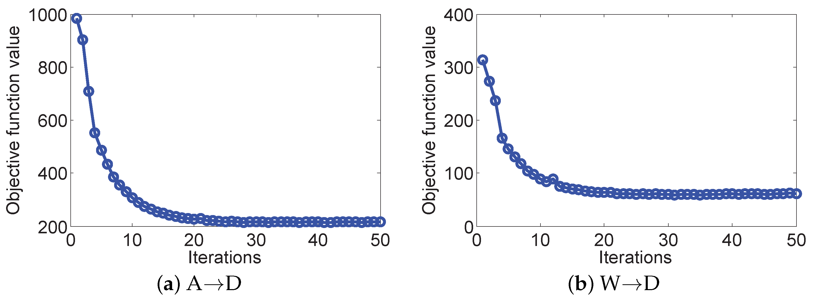
where , , , and are the solutions generated in the k-th iteration. We previously showed that the first condition is easy to obey. The second condition is hard to be proved directly, and thus in the section of the experiment we show that this condition can hold in real-world applications. Figure 3 displays the convergence curves of our method on two different cases. It can be seen that the object value decreases monotonically with the increase in the number of iterations. This demonstrates that the proposed optimization algorithm is efficient and has a fast convergence behavior, say within 20 iterations.
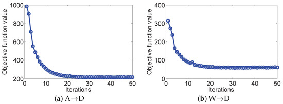
Figure 3.
Convergence curves of our method on different cases. (a) A→D with SURF feature and (b) W→D with CNN feature.
3.6. Connections to Existing Works
As discussed in Section 2, our proposed method significantly differs from previous transfer learning methods such as LTSL [2], RDALR [4], and TSD [3] in the following aspects.
(1) A great deal of work has been proposed for visual object classification, e.g., scene classification and image tagging [15,45] by transforming the data from different domains into the latent common subspace to reduce the distribution difference. Although these methods can push the data from different domains together, the data from different domains but with the same label cannot align together. Therefore, our proposed method uses matrix Q to transform the data from the original feature space into the latent common subspace for reducing the distribution discrepancy. More importantly, we impose the joint low-rank and sparse constraints on the reconstruction coefficient matrix to guarantee that: (a) the data from different domains can be closely interlaced; (b) the data from different domains but with the same label can be aligned together to seek the neighborhood to neighborhood reconstruction.
(2) Conventional transfer learning methods [8,22,46,47,48] mainly learn a transformation to reduce the distribution but ignore the classifier learning. In the proposed method, the new feature representation learning and classifier learning are integrated into the unified optimization framework. Thus, we can learn a suitable feature representation and use it as the input for learning the discriminative classifier parameter.
To our knowledge, LTSL [2] and RDALR [4] are most closely related to our RLCSL. For the clearness of comparison, the difference between these methods are as follows:
(1) Difference from LTSL [2] (lost local structure information): In LTSL, a unified transformation is used to transform the data from both the source and target domains into a common subspace where the discrepancy of the source and the target domains is decreased with a low-rank constraint, and the classification is performed in the common subspace. RLCSL first uses a transformation matrix to transform the data from both the source and target domains into the latent common subspace for eliminating or reducing the distribution discrepancy and simultaneously the classifier is learned from the latent common subspace by another transformation matrix. In this way, the common subspace learned by RLCSL is more discriminative to fit the labels than LTSL. In addition, in our RLCSL, the sparse constraint can effectively improve the discriminative ability of the new feature representation.
(2) Difference from RDALR [4]: In RDALR, only the source data are transformed into an intermediate subspace, which has too little freedom to pull the source domain close enough to the target domain. Moreover, when the source domain data are transformed into the target domain, the data of different subjects may overlap each other and thus it is difficult to separate them. In contrast, our method transforms both of them into a latent common subspace, which can make them close enough to each other. Additionally, a specific linear classifier is learned to ensure that they are separated as much as possible.
It is necessary to note that LTSL and RDALR only use the low-rank constraint to address the transfer learning problem which cannot guarantee that the data from the same subject in one domain may choose the data points of the same subject from another domain. By using the sparse constraint, RDALR tends to select the data points from different domains but the same subject for reconstruction. This is useful to find the discriminant structure of the data from different domains [3].
4. Experiments
In this section, we conducted massive experiments on three different data sets, i.e., object recognition, image classification, and text classification, to evaluate the classification performance of RLCSL.
4.1. Data Set Preparation
Text Data set: Reuters-21,578 [22,49] is a benchmark text corpora that is widely used for testing the performance of transfer learning. Reuters-21,578 is a complex text data set with many top and subcategories. The three largest top categories are orgs, people, and place, each of which is comprised of many subcategories.
Object Data set: Office is the visual domain benchmark data, including common object categories from three different domains, i.e., Amazon, DSLR, and Webcam. In this data set, each domain contains 31 object categories, such as laptop, keyboard, monitor, bike, etc., and the total number of images is 4652. In the Amazon domain, each category has 90 images on average while in DSLR or Webcam each category has 30 images on average. Caltech-256 is also a standard data set for object recognition, which has 30,607 images from 256 categories. In our experiments, the public Office + Caltech data sets released by Gong [50] are adopted. SURF features are extracted and quantized into an 800-bin histogram with codebooks computed with K-means on a subset of images from Amazon. Then the histograms are standardized by z-score. In sum, we have four domains: A (Amazon), D (DSLR), W (Webcam), and C (Caltech-256). In addition to the SURF feature, we also selected the convolutional neural network (CNN) feature to test the performance of different methods. For the CNN feature, eight layers with five convolutional layers and three fully connected layers of CNN were trained on the ImageNet in [51]. Our experiments used the output of the 6th layer with 4096 dimensionalities. More details of the architecture and training protocol can be found in [51].
Image Data set: MSRC and VOC2007 [52] are used in our experiments. The MSRC data set is released by Microsoft Research Cambridge, containing 4323 images labeled by 18 classes. The VOC2007 data set consists of 5011 images annotated with 20 concepts. These two data sets share six common semantic classes: airplane, bicycle, bird, car, cow, and sheep.
Table 3 shows the detailed introduction of these data sets.
Table 3.
Detailed information of different data sets (note the number in parentheses is the dimensionality).
4.2. Comparison Methods
In order to evaluate the validity of the proposed RLCSL method with different configurations of these data sets, we compared RLCSL with some competitive state-of-the-art methods including geodesic flow kernel (GFK) + NN [50], transfer component analysis (TCA) + NN [7], transfer subspace learning (TSL) + NN [42], low-rank transfer subspace learning (LDA) + NN (LTSL) [2], robust visual domain adaptation with low-rank reconstruction (RDALR) + NN [4], transfer feature learning with joint distribution adaptation (JDA) [53], scatter component analysis (SCA) [54], discriminative transfer subspace learning via low-rank and sparse representation (DTSL) [55], joint feature selection and subspace learning (FSSL) [56], transfer joint matching (TJM) for unsupervised domain adaptation [52], and 1-nearest neighbor classification (NN) and principle component analysis (PCA) + NN. In the experiment, TSL adopts Bregman divergence instead of maximum mean discrepancy (MMD) as the distance for comparing distributions. NN is chosen as the baseline classifier because there is no need for parameter tuning. Please note that partial experiments results are quoted from [54].
4.3. Experiments on the Office, Caltech-256 Data Sets
By randomly selecting 2 different domains as the source domain and target domain respectively, we constructed 12 different cross-domain object data sets, e.g., A→D, A→W, A→C, ⋯, C→W. The experimental results of single source domain and single target domain on these 12 cross-domain object data sets are shown in Table 4.
Table 4.
Classification accuracies (%) of different methods on the Office and Caltech-256 data sets.
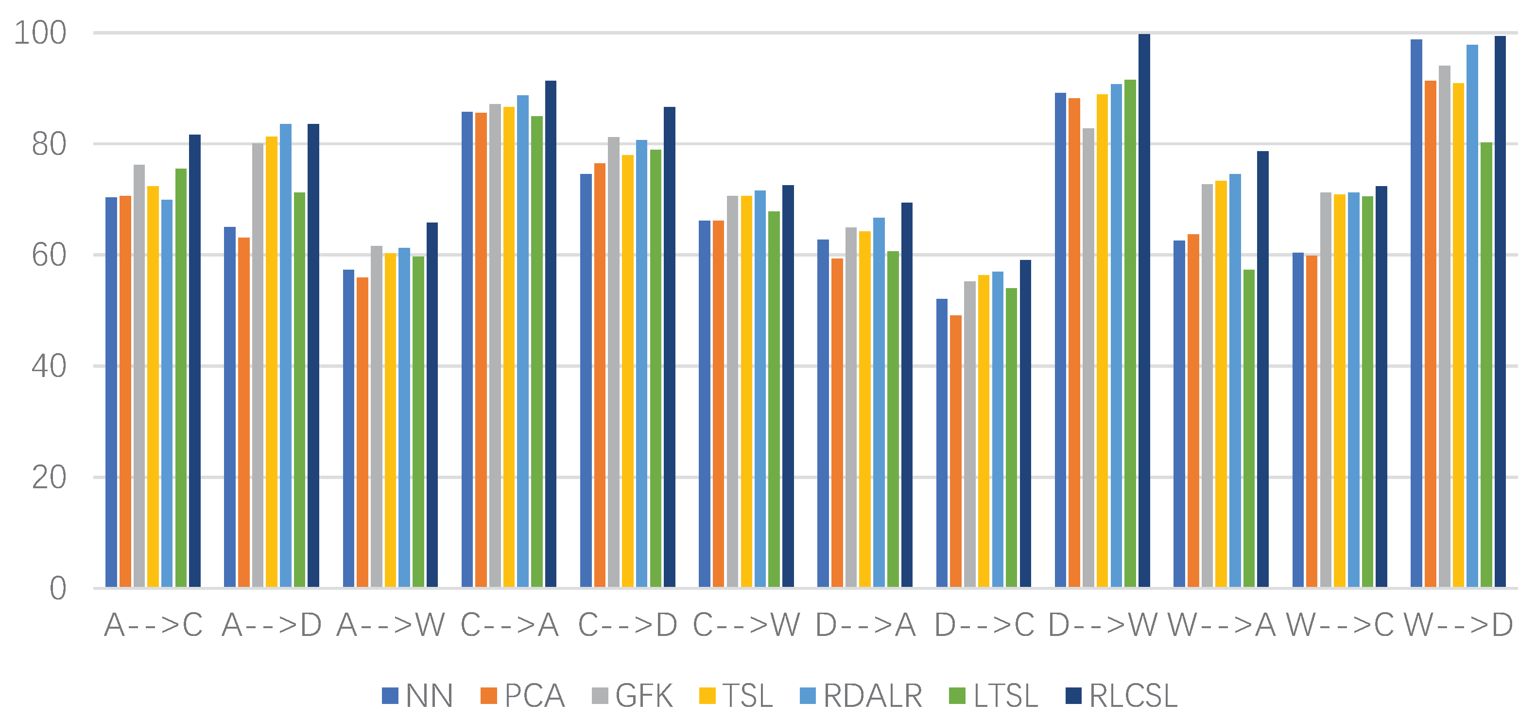
In order to evaluate the classification performance of the comparison methods and RLCSL better, we conducted the experiments of multiple sources domains vs. single target domain on the Office and Caltech 256 data sets. We randomly choose two subsets as the source domain while a single data set as the target domain. Thus, we also can construct 12 different cross-domain object data sets, e.g., AC→D, AC→W, ⋯, DW→C. The experimental results are shown in Table 5. From Table 4 and Table 5, the experimental results show that RLCSL is able to obtain good classification accuracies. Figure 4 provides the classification accuracy of different methods with the CNN feature. As shown in Figure 4, we can find that all methods obtain better classification results and our method is still the best competitor. The reason of supporting the excellent classification performance of RLCSL is twofold: the joint low-rank and sparse constraints can reduce the distribution discrepancy, plus the transferable feature representation learning and classification learning are integrated into the unified optimization objective. Thus, the proposed method can benefit from the high-level feature for improving classification accuracy. Although LTSL and RDALR use the low-rank constraint to learn the transferable feature representation, they separately learn the transferable feature representation and classifier. Therefore, the high-level feature, i.e., the semantic label is not directly related to the learning process in LTSL and RDALR. This also means that RLCSL can benefit from the high-level feature but LTSL and RDALR may not.
Table 5.
Classification accuracies (%) of multiple source domains vs single target domain on the Office and Caltech-256 data sets.
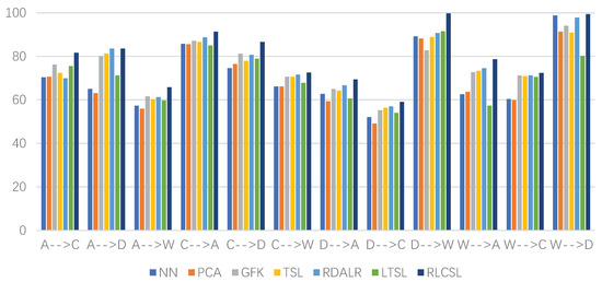
Figure 4.
Classification accuracies (%) of different methods on the Office and Caltech-256 data sets with CNN feature in which the Y-axis represents the classification accuracy and X-axis represents different cases.
4.4. Experiments on the Reuters-21,578 Data Set
For the Reuters-21,578 data set, we can generate six different cross-domain text data sets orgs → people (or → pe), people → orgs (pe → or), orgs → place (or → pl), place → orgs (pl → or), people → place (pe → pl), and place → people (pl → pe) by utilizing the three largest top categories. For the fairness of comparison, we directly adopted the preprocessed version of Reuters-21,578 provided by Long [49] (http://ise.thss.tsinghua.edu.cn/~mlong/, accessed on 31 December 2021). Table 6 shows the classification performance of different methods on the Reuters-21,578 data set. The results in Table 6 show the superiority of RLCSL with respect to classification performance.
Table 6.
Classification accuracies (%) of different methods on the Reuters-21,578 data set.
4.5. Experiments on the MSRC and VOC2007 Data Sets
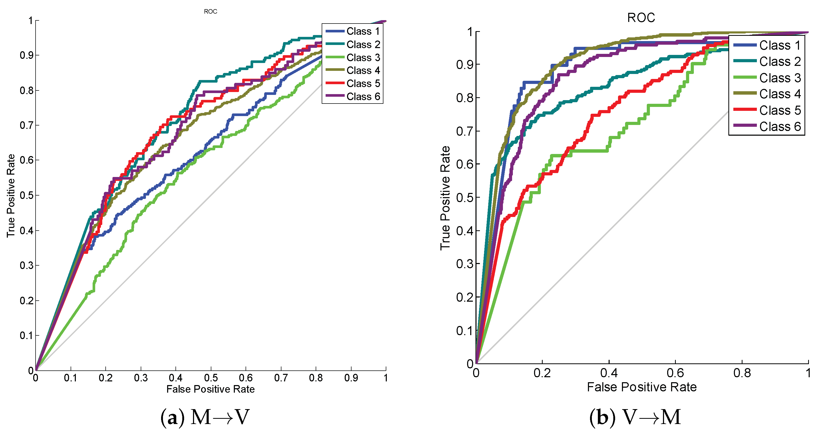
Following [52], for these two data sets, we constructed MSRC vs. VOC2007 (M→V) by choosing a total of 1269 images in MSRC as the source domain, and a total of 1530 images in VOC2007 as the target domain. Besides, we switched the data set with another data set: VOC2007 vs. MSRC (V→M). All the source and target domain images are uniformly rescaled to pixels in length, and extract 128-dimensional dense SIFT (DSIFT) features utilizing the VLFeat open-source package. Then K-means clustering is utilized to obtain a 240-dimensional codebook. As such, the training and test data are constructed to share the same label set and feature space. The classification results are shown in Table 7 in which our proposed method obtains the best classification result. Figure 5 gives receiver operating characteristic (ROC) curve on this data set from which we can see that class 2 and class 4 achieve the best classification performance on cases of M→V and V→M, respectively.
Table 7.
Classification accuracies (%) of different methods on the MSRC and VOC2007 data sets.
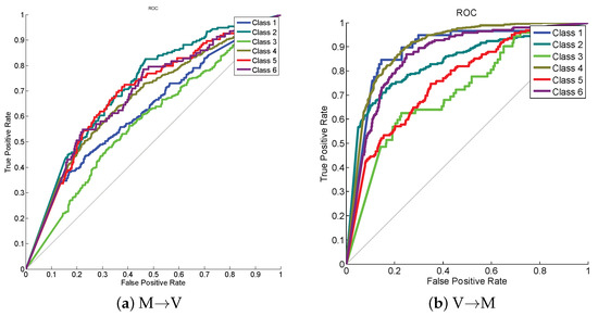
Figure 5.
ROC curves on cases of (a) M→V and (b) V→M.
The training time of different methods is shown in Table 8. The results in Table 8 show that the proposed method RLCSL obtains the third ranking in training time. The main reason may be that RLCSL takes a large amount of time to solve the joint low-rank and sparse optimization problem.
Table 8.
Time cost(s) of different methods on different data sets.
4.6. Visualization Analysis of Matrix Z
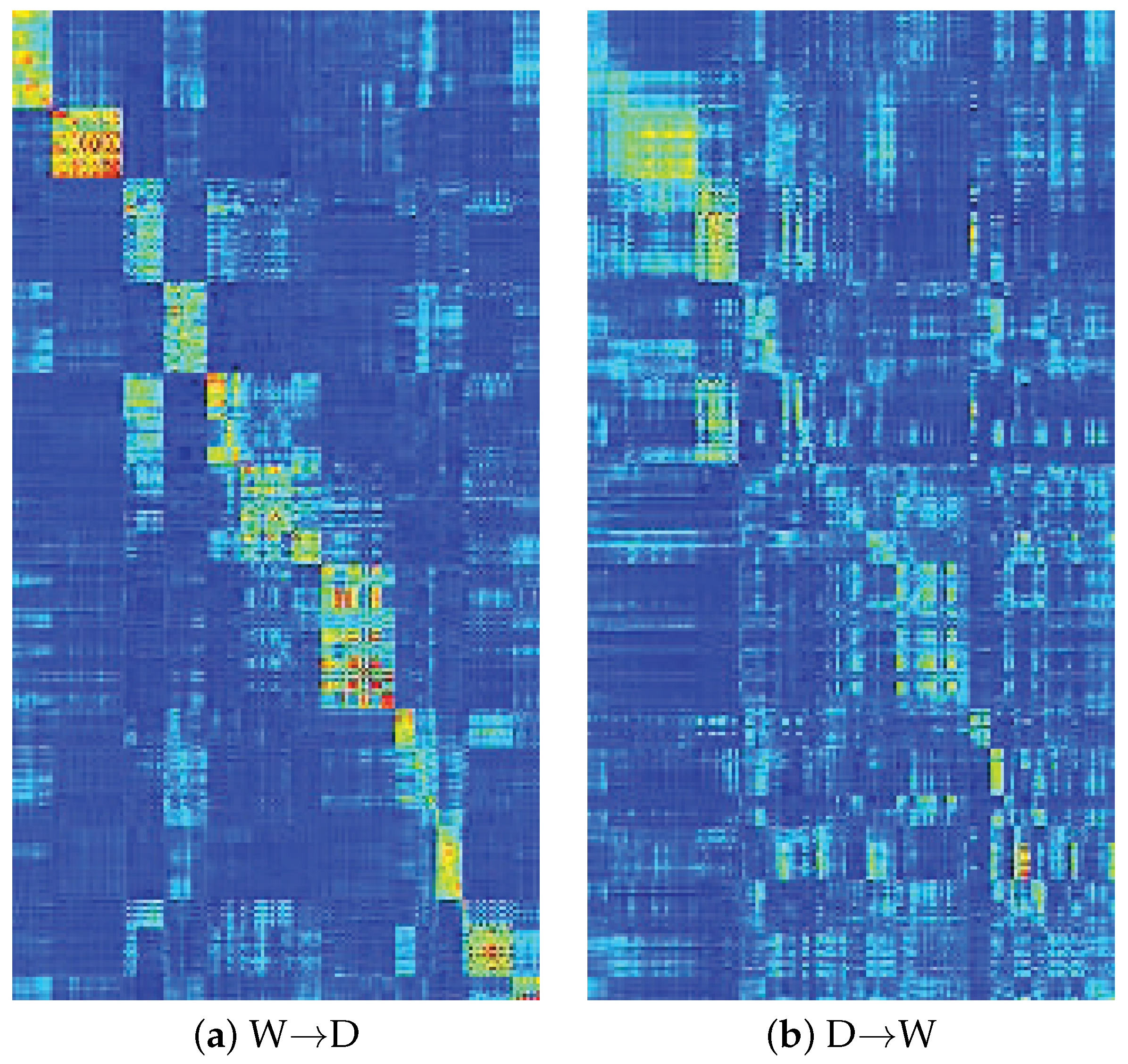
Figure 6 gives the visualization of matrix Z. It is obvious that the learned matrix Z is sparse and low-rank which means that although we used matrix H to replace matrix Z in our optimization algorithm, the algorithm finally satisfies constraint after algorithm convergence. We eventually obtain the sparse and low-rank reconstruction coefficient matrix Z that is very useful to align the data from different domains, which further confirms the motivation of our method from the view of optimization. In addition, we can see that the block-wise structure in matrix Z is somewhat obscure. The reason may be that the distribution discrepancy of data from different domains is not completely eliminated. However, the block-wise structure in matrix Z is very obvious in locations of many classes. This indicates that the data from different domains but with the same label can be aligned together and then the distribution discrepancy of different domains is reduced and representations of and are discriminative. In other words, the latent common subspace, i.e., Q can be used as an intermediate that can not only reduce the distribution discrepancy but also improve the discriminative ability of new data representation and . From this point, the latent common subspace is suitable for transfer learning and classifier learning.
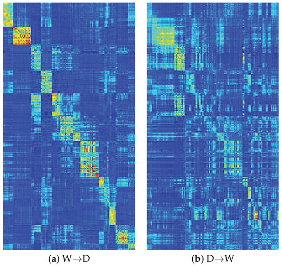
Figure 6.
Visualization of matrix Z on two different cases in which the case of W→D is performed on CNN feature and the case of D→W is performed on SURF feature.
4.7. Parameter Sensitivity
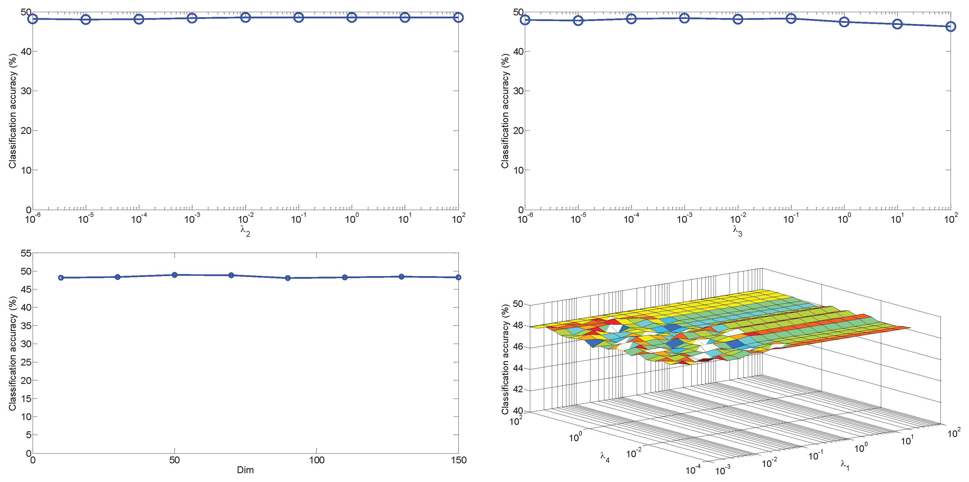
There are four parameters , , , and in our objective function. Specifically, and are used to balance the importance of the low-rank and sparse constraint terms. The goal of is to control the influence of noise and is used to avoid the problem of over-fitting. Theoretically, large values of or can make the reconstruction coefficient matrix Z more important in the proposed method. In our method, we always set for obtaining better experimental results. However, Figure 7 shows that both and have slight effects on the classification performance on the case of . We given different combinations of these two parameters from a reasonable discrete set in Figure 7, which indicates that the classification performance of our proposed method is roughly consistent over a wide range of values of these two parameters. For parameters and , we can see from Figure 7 that the classification accuracy of our proposed method is very robust to different settings provided the parameters are set in a feasible range. For dimensionality , we can see from Figure 7 that the proposed method is robust to the value of . From Figure 7, we can also find that it is an easy job to pick up a suitable parameters combination for the proposed method.
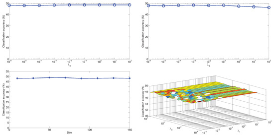
Figure 7.
The classification performance of our method vs. different parameters on the case of with SURF feature.
4.8. Ablation Studies
In order to study the proposed RLCSL deeply, we conducted the ablation studies to test the indispensability of each component of RLCSL by comparing RLCSL with four variants of RLCSL. The objective of the first variant is as follows
The goal of is to test the effectiveness of the low-rank constraint. The objective of the second variant is as follows
whose goal is to verify the effectiveness of the joint low-rank and sparse constraints. The objective of the third variant is as follows
whose goal is to verify the effectiveness of the sparse term (the main goal is to reduce the negative affect of noisy term). The objective of the fourth variant is as follows
whose goal is to test the effectiveness of sparse constraint.
The experimental results are shown in Figure 8. From the results in Figure 8, we can see that the low-rank constraint is more important than other terms on aligning data from the different domains ( is the second-best competitor). The experimental results also show that the sparse constraint, i.e., sparse constraint, also plays an important role in improving the classification accuracy ( is the third competitor). The sparse noisy term can reduce the effect of noisy term and thus it can improve the classification accuracy ( is the fourth competitor). When we removed the joint low-rank and sparse constraints the classification performance is relatively poor ( obtains the lower classification accuracy). Therefore, it is necessary to integrate all components into RLCSL for ensuring better classification performance.
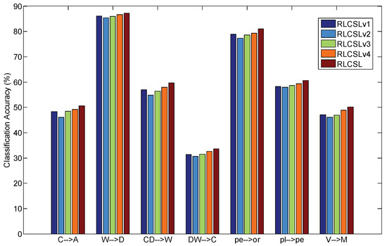
Figure 8.
Ablation studies of RLCSL.
5. Limitations
The limitations of the proposed method are as follows: (1) the dimension of latent common subspace needs to be set in advance although the algorithm is robust to the variation of its value; (2) the mathematical programming formulation is nonconvex. Although the convergence curve indicates that the proposed optimization algorithm has weak convergence properties, there is no strict theory to guarantee that the convergence behavior is always satisfied.
6. Conclusions
This paper proposes a novel robust latent common subspace learning method which utilizes the joint low-rank and sparse constraints to constrain the reconstruction coefficient matrix for obtaining a transferable and discriminative feature representation. Simultaneously, the latent common subspace is used as an intermediate that reduces the semantic gap between the low-level data representation and the high-level semantics. By integrating the classifier learning and latent common subspace learning into a unified framework, we learn a discriminative classifier parameter. The main difference between the proposed method and most related methods is shown in Table 9. The encouraging experimental results show the effectiveness of the proposed method. In the future, we are planning to extend our method to the semi-supervised transfer learning scenario and apply our proposed method into medical data analysis [57,58] for computer-aided medical diagnosis [59,60].
Table 9.
Comparison between most related works.
Author Contributions
Methodology, formal analysis, writing—original draft preparation, funding acquisition, S.Z.; formal analysis, investigation, writing—review, supervision, funding acquisition, W.S.; software, validation, and editing, visualization, writing—editing, P.K. All authors have read and agreed to the published version of the manuscript.
Funding
This research was funded by the Science and Technology Planning Project of Guangdong Province, China, under Grant 2019B110210002 and Grant 2019B020208001, the Educational Commission of Guangdong Province, China under Grant 2018GkQNCX076, the Key-Area Research and Development Program of Guangdong Province under Grant 2019B010121001 and Grant 2019B010118001, the National Key Research and Development Project under Grant 2018YFB1802400, and the National Natural Science Foundation of China (NSFC) under Grant U1911401.
Institutional Review Board Statement
Not applicable.
Informed Consent Statement
Not applicable.
Data Availability Statement
Not applicable.
Conflicts of Interest
The authors declare no conflict of interest.
References
- Xiao, M.; Guo, Y.H. Feature space independent semi-supervised domain adaptation via kernel matching. IEEE Trans. Pattern Anal. Mach. Intell. 2015, 37, 54–66. [Google Scholar] [CrossRef] [PubMed]
- Shao, M.; Kit, D.; Fu, Y. Generalized transfer subspace learning through low-rank constraint. Int. J. Comput. Vis. 2014, 109, 74–93. [Google Scholar] [CrossRef]
- Han, N.; Wu, J.; Fang, X.; Teng, S.; Zhou, G.; Xie, S.; Li, X. Projective Double Reconstructions Based Dictionary Learning Algorithm for Cross-Domain Recognition. IEEE Trans. Image Process. 2020, 29, 9220–9233. [Google Scholar] [CrossRef] [PubMed]
- Jhuo, I.H.; Liu, D.; Lee, D.T.; Chang, S.F. Robust visual domain adaptation with low-rank reconstruction. In Proceedings of the 2012 IEEE Conference on Computer Vision and Pattern Recognition, Providence, RI, USA, 16–21 June 2012; pp. 2168–2175. [Google Scholar]
- Han, N.; Wu, J.; Fang, X.; Wen, J.; Zhan, S.; Xie, S.; Li, X. Transferable linear discriminant analysis. IEEE Trans. Neural Netw. Learn. Syst. 2020, 31, 5630–5638. [Google Scholar] [CrossRef]
- Wu, X.; Chen, J.; Yu, F.; Yao, M.; Luo, J. Joint Learning of Multiple Latent Domains and Deep Representations for Domain Adaptation. IEEE Trans. Cybern. 2021, 51, 2676–2687. [Google Scholar] [CrossRef]
- Pan, S.J.; Tsang, I.W.; Kwok, J.T.; Yang, Q. Domain adaptation via transfer component analysis. IEEE Trans. Neural Netw. 2011, 22, 199–210. [Google Scholar] [CrossRef] [Green Version]
- Long, M.S.; Wang, J.M.; Ding, G.G.; Shen, D.; Yang, Q. Transfer Learning with Graph Co-Regularization. IEEE Trans. Knowl. Data Eng. 2014, 26, 1805–1818. [Google Scholar] [CrossRef] [Green Version]
- Zhuang, F.; Qi, Z.; Duan, K.; Xi, D.; Zhu, Y.; Zhu, Y.; Zhu, H.; Xiong, H.; He, Q. A Comprehensive Survey on Transfer Learning. Proc. IEEE 2021, 109, 43–76. [Google Scholar] [CrossRef]
- Fan, Z.Z.; Xu, Y.; Zhang, D. Local linear discriminant analysis framework using sample neighbors. IEEE Trans. Neural Netw. 2011, 22, 1119–1132. [Google Scholar] [CrossRef]
- Fang, X.; Xu, Y.; Li, X.; Fan, Z.; Liu, H.; Chen, Y. Locality and similarity preserving embedding for feature selection. Neurocomputing 2014, 128, 304–315. [Google Scholar] [CrossRef]
- Pan, S.J.; Kwok, J.T.; Yang, Q. Transfer learning via dimensionality reduction. In Proceedings of the Twenty-Third AAAI Conference on Artificial Intelligence (2008), Chicago, IL, USA, 13–17 July 2008; pp. 677–682. [Google Scholar]
- von Bünau, P.; Meinecke, F.C.; Kirúly, F.C.; Müller, K.R. Finding stationary subspaces in multivariate time series. Phys. Rev. Lett. 2009, 103, 214101. [Google Scholar] [CrossRef] [PubMed]
- Suykens, J. Data visualization and dimensionality reduction using kernel maps with a reference point. IEEE Trans. Neural Netw. 2008, 19, 1501–1517. [Google Scholar] [CrossRef] [PubMed] [Green Version]
- Wang, S.; Zhang, L.; Zuo, W.; Zhang, B. Class-specific reconstruction transfer learning for visual recognition across domains. IEEE Trans. Image Process. 2020, 29, 2424–2438. [Google Scholar] [CrossRef] [PubMed]
- Smeulders, A.W.M.; Worring, M.; Santini, S.; Gupta, A.; Jain, R. Content-based image retrieval at the end of the early years. IEEE Trans. Pattern Anal. Mach. Intell. 2000, 22, 1349–1380. [Google Scholar] [CrossRef]
- Roweis, S.T.; Saul, L.K. Nonlinear dimensionality reduction by locally linear embedding. Science 2000, 290, 2323–2326. [Google Scholar] [CrossRef] [Green Version]
- Cai, D.; He, X.F.; Han, J.W.; Huang, T. Graph Regularized Non-negative Matrix Factorization for Data Representation. IEEE Trans. Pattern Anal. Mach. Intell. 2011, 33, 1548–1560. [Google Scholar]
- Ma, Z.G.; Yang, Y.; Sebe, N.; Hauptmann, A. Knowledge adaptation with partially shared features for event detection using few examplars. IEEE Trans. Pattern Anal. Mach. Intell. 2014, 36, 1789–1802. [Google Scholar] [CrossRef]
- Pan, S.J.; Yang, Q. A survey on transfer learning. IEEE Trans. Knowl. Data Eng. 2010, 22, 1345–1359. [Google Scholar] [CrossRef]
- Ling, S.; Zhu, F.; Li, L.X. Transfer learning for visual categorization: A survey. IEEE Trans. Neural Netw. Learn. Syst. 2015, 26, 1019–1034. [Google Scholar] [CrossRef]
- Long, M.S.; Wan, J.M.; Ding, G.G.; Pan, S.J.; Yu, P.S. Adaptation Regularization: A General Framework for Transfer Learning. IEEE Trans. Knowl. Data Eng. 2014, 26, 1076–1089. [Google Scholar] [CrossRef]
- Jiang, J.; Zhai, C.X. Instance weighting for domain adaptation in NLP. In Proceedings of the 45th Annual Meeting of the Association Computational Linguistics, Prague, Czech Republic, 23–30 June 2007; pp. 264–271. [Google Scholar]
- Mihalkova, L.; Huynh, T.; Mooney, R. Mapping and revising markov logic networks for transfer learning. In Proceedings of the 22nd National Conference on Artificial Intelligence, Vancouver, BC, Canada, 22–26 July 2007; pp. 608–614. [Google Scholar]
- Raina, R.; Battle, A.; Lee, H.; Packer, B.; Ng, A. Self-taught learning: Transfer learning from unlabeled data. In Proceedings of the 24th International Conference on Machine Learning, Corvalis, OR, USA, 20–24 June 2007; pp. 759–766. [Google Scholar]
- Andreas, A.; Evgeniou, T.; Pontil, M. Convex multi-task feature learning. Mach. Learn. 2008, 73, 243–272. [Google Scholar]
- Kouw, W.; Loog, M. A Review of Domain Adaptation without Target Labels. IEEE Trans. Pattern Anal. Mach. Intell. 2021, 43, 766–785. [Google Scholar] [CrossRef] [PubMed] [Green Version]
- Gopalan, R.; Li, R.; Chellappa, R. Domain adaptation for object recognition: An unsupervised approach. In Proceedings of the 2011 International Conference on Computer Vision, Barcelona, Spain, 18–21 July 2011; pp. 999–1006. [Google Scholar]
- Hoffman, J.; Rodner, E.; Donahue, J.; Darrell, T.; Saenko, K. Efficient learning of domain-invariant image representation. arXiv 2013, arXiv:1301.3224. [Google Scholar]
- Wang, Z.; Song, Y.; Zhang, C. Transferred dimensionality reduction. In Machine Learning and Knowledge Discovery in Databases; Springer: New York, NY, USA, 2008. [Google Scholar]
- Yang, J.; Yan, R.; Hauptmann, A.G. Cross-domain video concept detection using adaptive svms. In Proceedings of the 15th ACM International Conference on Multimedia, New York, NY, USA, 25–29 September 2007; pp. 188–197. [Google Scholar]
- Bruzzone, L.; Marconcini, M. Domain adaptation problems: Adasvm classification technique and a circular validation strategy. IEEE Trans. Pattern Anal. Mach. Intell. 2010, 32, 770–787. [Google Scholar] [CrossRef] [PubMed] [Green Version]
- Chen, Y.; Wang, G.; Dong, S. Learning with progressive transductive support vector machine. Pattern Recognit. Lett. 2003, 24, 1845–1855. [Google Scholar] [CrossRef]
- Xue, Y.; Liao, X.; Carin, L.; Krishnapuram, B. Multi-task learning for classification with dirichlet process priors. J. Mach. Res. 2007, 8, 35–63. [Google Scholar]
- He, X.; Yan, S.; Hu, Y.; Niyogi, P.; Zhang, H. Face recognition using Laplacian faces. IEEE Trans. Pattern Anal. Mach. 2005, 27, 328–340. [Google Scholar]
- He, X.; Cai, D.; Yan, S.; Zhang, H.J. Neighborhood preserving embedding. In Proceedings of the Tenth IEEE International Conference on Computer Vision (ICCV’05), Beijing, China, 17–21 October 2005; pp. 1208–1213. [Google Scholar]
- Cai, D.; He, X.; Han, J. Isometric projection. In Proceedings of the 22nd National Conference on Artificial Intelligence, Vancouver, BC, Canada, 22–26 July 2007; pp. 528–533. [Google Scholar]
- Chen, H.T.; Chang, H.W.; Liu, T.L. Local discriminant embedding and its variants. In Proceedings of the 2005 IEEE Computer Society Conference on Computer Vision and Pattern Recognition (CVPR’05), San Diego, CA, USA, 20–25 June 2005; pp. 846–853. [Google Scholar]
- Liu, F.; Zhang, G.; Zhou, J. Heterogeneous Domain Adaptation: An Unsupervised Approach. IEEE Trans. Neural Netw. Learn. Syst. 2020, 31, 5588–5602. [Google Scholar] [CrossRef] [Green Version]
- Ding, Z.; Fu, Y. Robust transfer metric learning for image classification. IEEE Trans. Image Process. 2017, 26, 660–670. [Google Scholar] [CrossRef]
- Liu, G.; Lin, Z.; Yan, S.; Sun, J.; Yu, Y.; Ma, Y. Robust recovery of subspace structures by low-rank representation. IEEE Trans. Pattern Anal. Mach. Intell. 2013, 35, 171–184. [Google Scholar] [CrossRef] [Green Version]
- Si, S.; Tao, D.C.; Geng, B. Bregman divergence-based regularization fro transfer subsapce learning. IEEE Trans. Knowl. Data Eng. 2010, 22, 929–942. [Google Scholar] [CrossRef]
- Eckstein, J.; Bertsekas, D.P. On the Douglas Rachford splitting method and the proximal point algorithm for maximal monotone operators. Math. Program. 1992, 55, 293–318. [Google Scholar] [CrossRef] [Green Version]
- Lin, Z.C.; Liu, R.S.; Su, Z.X. Linearized alternating direction method with adaptive penalty for low rank representation. Adv. Neural Inf. Process. Syst. 2011, 24, 612–620. [Google Scholar]
- Li, X.; Guo, Y.H. Latent semantic representation learning for scence classification. In Proceedings of the International Conference on Machine Learning, Beijing, China, 21–26 June 2014; pp. 532–540. [Google Scholar]
- Ling, X.; Dai, W.; Xue, G.-R.; Yang, Q.; Yu, Y. Spectral domain-transfer learning. In Proceedings of the 14th ACM SIGKDD International Conference on KNOWLEDGE Discovery and Data Mining, Las Vegas, NV, USA, 24–27 August 2008. [Google Scholar]
- Wang, C.; Mahadevan, S. Heterogeneous domain adaptation using manifold alignment. In Proceedings of the Twenty-Second International Joint Conference on Artificial Intelligence, Barcelona, Spain, 16–22 July 2011. [Google Scholar]
- Shi, X.; Liu, Q.; Fan, W.; Yu, P.S. Transfer across completely different feature spaces via spectral embedding. IEEE Trans. Knowl. Data Eng. 2013, 25, 906–918. [Google Scholar] [CrossRef]
- Long, M.S.; Wang, J.M.; Sun, J.G.; Yu, P.S. Domain Invariant Transfer Kernel Learning. IEEE Trans. Knowl. Data Eng. 2015, 27, 1519–1532. [Google Scholar] [CrossRef]
- Gong, B.; Shi, Y.; Sha, F.; Grauman, K. Geodesic Flow Kernel for Unsupervised Domain Adaptation. In Proceedings of the 2012 IEEE Conference on Computer Vision and Pattern Recognition, Providence, RI, USA, 16–21 June 2012; pp. 2066–2073. [Google Scholar]
- Krizhevsky, A.; Sutskever, I.; Hinton, G.E. ImageNet classification with deep convolutional neural networks. Adv. Neural Inf. Process. Syst. 2012, 25, 1097–1105. [Google Scholar] [CrossRef]
- Long, M.S.; Wang, J.M.; Ding, G.G.; Sun, J.G.; Yu, S. Transfer Joint Matching for Unsupervised Domain Adaptation. In Proceedings of the IEEE Conference on Computer Vision & Pattern Recognition, Columbus, OH, USA, 23–28 June 2014; pp. 1410–1417. [Google Scholar]
- Long, M.S.; Wang, J.M.; Ding, G.G.; Sun, J.G.; Yu, P.S. Transfer Feature Learning with Joint Distribution Adaptation. In Proceedings of the IEEE International Conference on COMPUTER Vision, Sydney, Australia, 1–8 December 2013; pp. 2200–2207. [Google Scholar]
- Ghifary, M.; Balduzzi, D.; Kleijn, W.; Zhang, M. Scatter Component Analysis: A Unified Framework for Domain Adaptation and Domain Generalization. IEEE Trans. Pattern Anal. Mach. Intell. 2017, 39, 1414–1430. [Google Scholar] [CrossRef] [Green Version]
- Xu, Y.; Fang, X.; Wu, J.; Li, X.; Zhang, D. Discriminative transfer subspace learning via low-rank and sparse representation. IEEE Trans. Image Process. 2016, 25, 850–863. [Google Scholar] [CrossRef]
- Gu, Q.; Li, Z.; Han, J. Joint feature selection and subspace learning. In Proceedings of the International Joint Conference on Artificial Intelligence, Catalonia, Spain, 16–22 July 2011. [Google Scholar]
- Shoeibi, A.; Khodatars, M.; Jafari, M.; Moridian, P.; Rezaei, M.; Alizadehsani, R.; Khozeimeh, F.; Gorriz, J.M.; Heras, J.; Panahiazar, M.; et al. Applications of Deep Learning Techniques for Automated Multiple Sclerosis Detection Using Magnetic Resonance Imaging: A Review. Comput. Biol. Med. 2021, 136, 104697. [Google Scholar] [CrossRef]
- Khodatars, M.; Shoeibi, A.; Sadeghi, D.; Ghaasemi, N.; Jafari, M.; Moridian, P.; Khadem, A.; Alizadehsani, R.; Zare, A.; Kong, Y.; et al. Deep Learning for Neuroimaging-based Diagnosis and Rehabilitation of Autism Spectrum Disorder: A Review. Comput. Biol. Med. 2021, 139, 104949. [Google Scholar] [CrossRef]
- Shoeibi, A.; Sadeghi, D.; Moridian, P.; Ghassemi, N.; Heras, J.; Alizadehsani, R.; Gorriz, J.M. Automatic Diagnosis of Schizophrenia Using EEG signals and CNN-LSTM Models. arXiv 2021, arXiv:2109.01120. [Google Scholar] [CrossRef] [PubMed]
- Sadeghi, D.; Shoeibi, A.; Ghassemi, N.; Moridian, P.; Khadem, A.; Alizadehsani, R.; Teshnehlab, M.; Gorriz, J.M.; Nahavandi, S. An Overview on Artificial Intelligence Techniques for Diagnosis of Schizophrenia Based on Magnetic Resonance Imaging Modalities: Methods, Challenges, and Future Works. arXiv 2021, arXiv:2103.03081. [Google Scholar]

Publisher’s Note: MDPI stays neutral with regard to jurisdictional claims in published maps and institutional affiliations. |
© 2022 by the authors. Licensee MDPI, Basel, Switzerland. This article is an open access article distributed under the terms and conditions of the Creative Commons Attribution (CC BY) license (https://creativecommons.org/licenses/by/4.0/).