Abstract
This study designs a trigger to determine the number of layers of a multi-layer adaptive Kalman filter and applies it to optoelectronic infrared payload system vision. This feature reduces the number of mechanically stabilized motors, equipment weight, CPU resources, and power for an electro-optical infrared payload system. The goal is to reduce the traditional use of multiple gyroscopes to perform calibration measurements on different gimbal frames by this design. In this study, mathematical modeling was carried out for the three-axis, three-frame camera stabilizer system, and the system foundation without motor and gimbal frame was established to achieve aperture-type camera mode. The exposure of the drone’s payload structure outside the aircraft can be reduced. This study provides the adaptive Kalman filter with the offset parameters of the camera image Minimum Output Sum of Squared Error and the three-axis degrees of freedom vector and angle data on the gyroscope. By using the image processing unit, the offset was corrected at each frame per second. The experimental results show that under the same hardware, failure limit and camera field of view constraints. The processing time by this method was compared to the traditional frame correction and full image stabilization methods. The results show that the proposed method can shorten 6 microseconds under the traditional method and can be used to provide lower power consumption, lower image delay, and a larger viewing angle range.
1. Introduction
Globally, in response to the technological advancement of drone micro-electromechanical systems, drone costs have fallen sharply. Applications of optoelectronic payloads and stabilizers become a standard component. Optoelectronic payloads are detection devices installed on servo-stabilized systems on moving carriers such as drones and track ground or air targets based on boresight stabilization technology. With the varying attitude angle of the carrier, the gyroscope’s photoelectric payload can be moved without interference from the carrier, stabilizing the picture and ensuring the detection equipment on the photoelectric payload. It can be found that optoelectronic payloads for drones have the advantage of key components in the drone market. Therefore, from 2016 to 2018, many solutions were obtained due to the microchip processing speed and data amount increased. It causes many different applications of optoelectronic payloads used in various military and civilian fields. As the speed of the processor increases and the amount of data processing is larger. The ability to perform calculations on images and signals simultaneously in one processor emerges is required. The traditional advantages of mechanical processing are gradually reduced, and instead, the image stabilization processing is performed by the image and the mechanical gimbal frame at the same time. Image processing research is the basis of this method. It can greatly increase the processing efficiency and reduce the use of the hardware gimbal frame. It further reduces the weight and resource consumption of image stabilization and can further utilize one processor to complete multiple tasks in the traditional method. The performance evaluation index of the photoelectric payload is the reliability of the data captured by the optical sensor. Therefore, the reliability of the data captured by the sensor is a key issue. Ref. [1] proposed an adaptive unscented Kalman filter for target tracking with time-varying noise covariance based on multi-sensor information fusion. An innovative optimal information fusion methodology is proposed based on adaptive and robust unscented Kalman filter (UKF) for multi-sensor nonlinear stochastic systems. Based on the linear minimum variance criterion, this multi-sensor information fusion method has a two-layer architecture: at the first layer, a new adaptive UKF scheme for the time-varying noise covariance was developed and served as a local filter to improve the adaptability together with the estimated measurement noise covariance by applying the redundant measurement noise covariance estimation, which is isolated from the state estimation; the second layer is the fusion structure to calculate the optimal matrix weights and gives the final optimal state estimations. Based on the hypothesis testing theory with the Mahalanobis distance, the new adaptive UKF scheme utilizes both the innovation and the residual sequences to adapt the process noise covariance timely. The results of the target tracking simulations indicate that the proposed method is effective under the condition of time-varying process-error and measurement noise covariance. Ref. [2] proposed the design of a stability control system for pan, tilt, and roll. The traditional gyro stabilization control method uses the angle information obtained by the gyro to extend the Kalman Filter and then corrects the position of the three-degree-of-freedom velocity integration in the original space [3]. The value is provided to calculate the parameters of the controller, and the angle information can be converted into a unit pulse (Pulse Width Modulation, PWM) signal to the MOSFET to generate a higher voltage to the motor. Ref. [4] uses a fixed-wing UAV to implement an automatic tracking system design. Reference [5] analyzed the various error sources of the three-axis gimbal, used the accuracy of the gyro error model to calibrate the accuracy, and established the photoelectric payload and the gyro model error equation. However, the actual internal error of the controller includes: gyro accuracy error, acceleration caused by gyro angle error, motor response time delay, payload vibration, and image scanning frequency resonance [6,7]; the above four items cause the final imaging image to be unclear or fuzzy. Key factors proposed a fuzzy PID control algorithm to control the operational stability of the photoelectric payload. However, updating the accuracy of the gyroscope causes a serious burden on the private sector. Acceleration caused by the gyro angle error can be corrected in real-time by setting the spatial position of one axis in the middle of the three-axis degrees of freedom as a constant. References [3,8] reposed a PTZ controller design method for UAV’s own motion compensation. By analyzing the effects of translation and rotation movement of UAV on the imaging of the target in the image plane, the relationship between the angular velocity of the body and the angular velocity of the PTZ attitude. In order to compensate for the change in the camera’s boresight caused by the UAV’s own motion, the position of the target in the image plane is used to correct the camera tracking error. In this paper, applied to the electro-optical infrared payload system’s vision offset function, the multiple layer Kalman Filter characteristic [9] was used to analyze the filter inertial measurement unit and design a trigger to set up the layer number of Kalman Filter [10]. This function can decrease the electro-optical infrared payload system’s number of stabilized motors, the weight of the device, central processing unit resource, and power. In this research, an illustrated example of a three-axis, three-gimbal system was analyzed by mathematical and simulation inertial measurement unit vibration. Three-axis degrees of freedom vector and gimbal motion data obtained by Kalman filter were provided to the graphics processing unit for offsetting each frame [10,11]. However, none of the studies mentioned above can be optimized for the efficiency of image stabilization. Additionally, the constraints of the main research are based on the design of the existing hardware. The fundamental problem is not substantially solved, and the response of the motor of the ring frame is lower due to the physical limit. Less response performance means that a powerful motor and lower energy consumption are required. The stabilization of the image only assists the system. Therefore, based on the literature [9,10,11], this study designs the input of the adaptive Kalman filter and combines the image tracking technology of [7] to improve the image quality. The goal was to use the proposed method to reduce the dependence of the optoelectronic payload driven by the motor. Ref. [12] proposed a dual-optimized adaptive Kalman filtering algorithm based on bp neural network and variance compensation for laser absorption spectroscopy. The analysis and design of a dual-optimized adaptive Kalman filtering (DO-AKF) algorithm based on back propagation (BP) neural network and variance compensation was developed for high-sensitivity trace gas detection in laser spectroscopy [13,14]. The BP neural network was used to optimize the Kalman filter (KF) parameters. Variance compensation was introduced to track the state of the system and to eliminate the variations in the parameters of dynamic systems. The proposed DO-AKF algorithm showed the best performance compared with the traditional multi-signal average, extended KF, unscented KF, KF optimized by BP neural network (BP-KF), and KF optimized by variance compensation (VC-KF) [15]. The optimized DO-AKF algorithm was applied to a QCL-based gas sensor system for an exhaled CO analysis [16]. The experimental results revealed a sensitivity enhancement factor of 23. The proposed algorithm can be widely used in the fields of environmental pollutant monitoring, industrial process control, and breath gas diagnosis.
The above mainly describes the design improvement and analysis of the EKF. The improvement of this algorithm was also used on UAVs, such as in reference [17]. A UAV swarm navigation using dynamic adaptive Kalman filter and network navigation was proposed. Ref. [18] also proposed a multi-sensor fusion based on adaptive Kalman filtering. The optimal performance of the conventional Kalman filters is not guaranteed when there is uncertainty in the process and measurement noise covariances. In this paper, in order to reduce the effect of noise covariance uncertainty, the Fuzzy Adaptive Iterated Extended Kalman Filter (FAIEKF) and Fuzzy Adaptive Unscented Kalman Filter (FAUKF) are proposed to overcome this drawback. The Proposed FAIEKF and FAUKF were applied to fuse signals from Global Positioning System (GPS) and Inertial Navigation Systems (INS) for the autonomous vehicles’ navigation. In order to validate the accuracy and convergence of the proposed approaches, results obtained by FAUKF and FAIEKF were compared to the Fuzzy Adaptive Extended Kalman Filter (FAEKF), Extended Kalman Filter (EKF), Unscented Kalman Filter (UKF), and Iterated Extended Kalman Filter (IEKF). The simulation results illustrate superior performance. It can be seen that the design and improvement of EKF are very common on UAVs. This research mainly focuses on the integration and optimization of image stabilization and UAV photoelectric stabilization systems. Ref. [10] showed a modified unscented Kalman filter using modified filter gain and variance scale factor for highly maneuvering target tracking. It improved the low tracking precision caused by lagged filter gain or imprecise state noise when the target highly maneuvers; therefore, a modified unscented Kalman filter algorithm based on the improved filter gain and adaptive scale factor of state noise was presented. In every filter process, the estimated scale factor is used to update the state noise covariance, and the improved filter gain is obtained in the filter process of unscented Kalman filter (UKF) via predicted variance, which is similar to the standard Kalman filter. Simulation results show that the proposed algorithm provides better accuracy and ability to adapt to the highly maneuvering target compared with the standard UKF. Ref. [8] proposed a dynamic Siamese network with an adaptive Kalman filter for object tracking in complex scenes. It solved the problem that the tracking accuracy of a fully-convolutional Siamese network (SiamFC) in complex scenes such as similar object interference, fast-moving, and appearance change is not good. A new object tracker based on a dynamic template updating strategy and the re-location mechanism based on the adaptive Kalman is proposed. In order to suppress the object interference and overcome the instability of fast-moving object tracking, an adaptive Kalman filter method was designed to change the selection method of search region and select the bounding box of the object closest to the predicted position. For the adaptation of appearance change, the high-confidence tracking results are fused with the initial template to dynamic update the template. Compared with the traditional Kalman filter, the expectation of residual error for the adaptive Kalman filter method can be controlled in a low range by the adjustment of the gain online. The introduction of the adaptive Kalman-based re-location mechanism improves the discriminative ability of SiamFC in the interference scene. With the dynamic template updating strategy, the tracker obtains strong generalization capability to adapt to the appearance change of the tracking target. It was demonstrated that the proposed method performs real-time object tracking at the speed of 43 fps and achieves competitive performance on OTB, VOT, and TC128 datasets compared with other state-of-the-art trackers.
The above research shows that the trend of the current technology is gradually changing from separate motor and image stabilization to pure gyro image stabilization. However, the above literature also shows that it is very unwise to use the gyroscope for image stabilization directly, and the noise on the gyroscope still has a large deviation even after traditional filtering. Therefore, how to use the gyroscope on the drone to perform image stabilization more effectively is a key issue.
This study shows the completion of the coordinate analysis of photoelectric gimbal payload and the preliminary description of coordinates, and the analysis was carried out under the assumption that variables such as material deformation are not considered. Mainly, the Minimum Output Sum of Squared Error (MOSSE) and Fully-Convolutional Siamese Networks (SiamFC) extraction methods of images were firstly established for theoretical establishment. The tracked target was then extracted relative to the error variable in the image. The theory of adaptive extended Kalman filter was established and described. Then substitute the variables were extracted by MOSSE and SiamFC. The actual hardware was verified first and then verified on different devices. The image error should be lower than one pixel, and the steady-state error of the gyroscopes in the experimental should be lower than 100 LSB/°/s. The key experimental data related to this study were extracted and shown in the following sections of the result and conclusion. Table 1 shows the relevant abbreviations and symbols used in the following.

Table 1.
Definition of Symbols.
2. Material and Method
2.1. Coordinate Analysis of Photoelectric Gimbal Payload
In this paper, it is assumed that the platform and the carrier are rigidly connected, that is, regardless of the damping effect between the platform base and the carrier. Therefore, the base coordinate system is considered to be the carrier coordinate system in the following analysis. As shown in Figure 1, the three-axis, three-frame gimbal stabilizer can be divided into vibration reduction system (defined as coordinate system 0), yaw frame (defined as coordinate system 1), pitch frame (defined as coordinate system 2), and roll frame (defined as the coordinate system 3) and other four parts, including the rotation angle of the yaw axis, the rotation angle of the tilt axis, the rotation angle of the roll axis, and the distance from the center point of the pitch frame to the motor of the roll frame. The distance is the vertical distance from the center point of the pitch frame to the position where the sensor is placed in the roll frame and the horizontal distance from the left end of the lower damping plate to the coordinate system (0). The structure is connected by three rotating joints, and each joint is driven by a motor; the yaw axis motion, pitch axis motion, and roll axis motion are controlled separately. When the carrier is vibrated or tilted by the external environment, the inertial measurement unit (IMU) installed on the rolling frame obtains the frame deviation. After calculation by the control algorithm, it outputs a compensation signal to drive the motor to generate a balanced torque so that the stabilizer eliminates deviation and maintains the horizontal stability of the boresight.
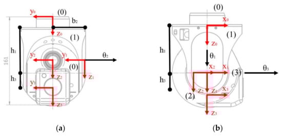
Figure 1.
Proposed spherical gimbal: (a) side view and (b) front view.
The mathematical modeling of the spherical gimbal in Figure 1 is derived in the following. The mechanism of the gimbal is composed of an anti-vibration plate, i.e., yaw frame, pitch frame, and roll frame, and each frame motion is driven by a motor. In order to analyze the dynamics of the gimbal, components of the gimbal are named as a sub-coordinate system, where the anti-vibration plate is denoted as coordinate system 0, and the frames of yaw, pitch, and roll are denoted as coordinate system 1, 2, and 3, respectively. As shown in Figure 2, is rotation angular of yaw axis, is rotation angular of pitch axis, is rotation angular of roll axis, is the minimum distance between yaw axis and motor of roll axis, is the minimum distance between anti-vibration plate and pitch axis, is the minimum distance between pitch axis and gyroscope sensor, and is the radius of anti-vibration plate. The motion of the spherical gimbal is measured by an inertial measurement unit (IMU) and is controlled by three motors to stabilize the aerial photography. The relative motion of each coordinate system can be obtained. Cartesian coordinates of systems 0, 1, 2, and 3 are defined as , , , and , respectively. The relative geometric relationship of coordinate system 0 and coordinate system 3 can be given as (1).
where and for are defined. Therefore, we have . Here, based on (1), the required command can be calculated, i.e., , , and , by an appropriate control system.
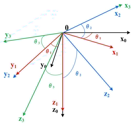
Figure 2.
Relative motion of each coordinate system.
2.2. MOSSE and SiamFC
In 2010, David S. B. proposed visual object tracking using adaptive correlation filters, which mentioned the error least square sum filter method [7]. The response represents the outer product of and the filtering model as given in (2).
Therefore, for the fastest response, the filtering model should be designed. Based on the Fast Fourier Transform (FFT) proposed by David S. B. [7], (2) can be written as (3).
Then the model can be obtained. However, the actual target locking and tracking process must take into account the deformation of the target’s appearance or the appearance of the image due to the rotation of the target. Therefore, multiple images of the target need to be accessed as a reference to improve the robustness of the filter model. Thus, the above formula (3) can be transformed into (4) and (5).
The input samples and the input features are generated through the Gaussian distribution. The value of the filter can be calculated after obtaining the training samples. Note that the sampling pixels of , , and are given the same. In order to improve the robustness of the filter in the environment of target type change or contrast and brightness change interference, based on [7], we have , and and are given as (6) and (7), respectively.
where are update parameters, including the gray-scale gain and when filtering are the above, respectively, and the updated variables are added to the loop when the image is mutated. The MOSSE image is tracked after real-time identification, and the feature image can be scanned in real-time without the need to build a model for the target. Because the traditional color binarization feature process is fast, it is easy to cause the recognition feature to fail at night or when the sensor does not invent a visible target. For other processes, the output range with naive filtering is too large to identify the feature position. For UMACE filtering, the output feature result has the highest accuracy, but it takes too much time to cause excessive frame loss. Such that the frames cannot be connected smoothly. The number of images that can be provided per unit time is the least. The MOSSE filtering results are similar, but the visible and thermal image fuzzy recognition is similar to the UMACE results. Using too much memory causes a loss of frame numbers.
In this study, the image captured by the optical payload is used to perform the MOSSE filtering on the pixels between 100 × 100 pixels at the position of four points in three-quarters of a pixel, as shown in Figure 3. The four point positions averaged the ideal sight center coordinates of the previous frame that was displaced due to the shock and averaged the position information of this shock and the feed-forward value in the motion control card to the position information of the next frame. The ability to approach real-time control is very high, so MOSSE is used for tracking and identification.
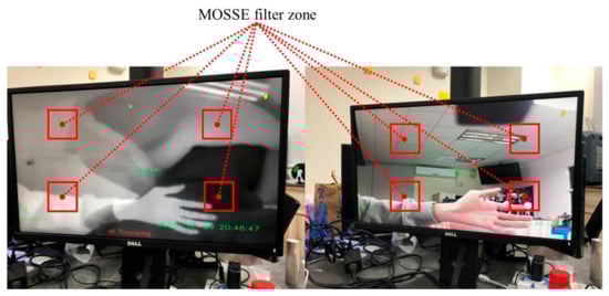
Figure 3.
MOSSE filter zone and SiamFC zone.
In Figure 4, is the initial target template for domain tracking and is the search area in the nth frame. An end-to-end Siamese network model is trained using fully connected layers and predefined learning methods in SiamFC. The image on the current frame and the search area are the inputs to SiamFC. The features of and in the feature space are extracted and make correlation connections. Note that the symbol of is represented as the product operator.
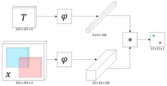
Figure 4.
Siam-FC structure.
The parameter of denotes a signal that takes value in all locations. The parameter is the feature extractor in the SiamFC. The function of is the correlation operation and is represented as the response map. The score means the similarity between the image template and the searching region. The position with maximum value in corresponds to the location of the target. In order to realize real-time tracking, the feature extractor is usually used based on a convolutional neural network such as AlexNet [10].
It is well known that Kalman filtering belongs to an autoregressive filter. The largest flaw originally designed must be applied to systems that conform to the Gaussian distribution, and extended Kalman filtering (EKF) can be used in nonlinear dynamic systems and discrete data collection. The key five types of EKF can be shown in (9)–(13).
where is given. The best quality control amount is based on the state of the top. At present, only the average value is calculated. When the Gaussian noise is 0, the second term can be set to 0. At the same time, the Kalman gain can be calculated by the squared difference of the predicted value, and the predicted value and the measured value are simultaneously calculated. The final Kalman gain is calculated by the squared difference of the proportionality factor, and the predicted value and the squared difference of the state are also obtained. At the same time, the measured value of the state is also obtained. At this time, the estimated state of the state can be calculated through the Kalman gain. The higher the reliability of the measured value of the system. Single-layer Kalman filtering was used to perform triaxial image rotation and vertical and horizontal movement.
2.3. Object Tracking with Adaptive EKF
Object tracking is a process involving time and space dimensions. The position contains the time trajectory information of the target. Therefore, the Kalman filter is used to integrate the temporal trajectory information of the target with the tracker, but it has obvious flaws when tracking. The Kalman filter tracking stabilization based on the mathematical model is precisely sufficient. Incorrect models and external disturbances can lead to loss of accuracy and even filter divergence. Kalman gain tends to stabilize when the Kalman filter reaches a steady state. If the target state changes suddenly, the Kalman filter will not be able to adjust the gain quickly, and the filter will diverge. The extended Kalman filter is used especially in the condition of only IMU output. Unlike using a Kalman filter in a simulation. The noise caused by the actual IMU output or the lack of proper high-frequency vibration isolation can easily cause the IMU to generate serious noise. This easily leads to a serious failure of the Kalman filter, and even the gain approaches zero. Based on this problem, this study provides a new method to suppress interference then overcome non-stabilization when the object moves too fast, or vibration isolation is incomplete. By using the adjustment factor, it is ensured that the filter gain matrix can be adjusted in time and the residual signals at different times are close to quadrature. Thus, the robustness of model tracking and the ability to adapt to target state mutation is obtained. The traditional Kalman filter has two update processes, time update and observation update. Time updates are mainly used for system predictions such as state and covariance predictions. The observation update includes the calculation of Kalman gain, state update, and covariance update, which is called the correction phase. The state is observed and used to correct the predicted value during the system prediction process. The state prediction can be expressed as (14)
where is a prediction of the previous state, is the state transition matrix, is the system parameter, is the control quantity of the process at the time . The state of the Kalman filter was formed by target positions and velocities . The residual at time can be expressed as (15). is observation at time . The parameter is the observation matrix. The covariance prediction process is used to predict the state as (16)
where is covariance prediction of state , and is the covariance matrix of the system process. The parameter is the adjustment factor for when the Kalman filter is given. First, the Kalman gain of state update and covariance update is calculated to obtain the current state observation value. State updates can be achieved through current optimal state estimates of predicted values, observed values, and gains. The Kalman gain can be defined as (17). is Kalman gain and is the covariance matrix of the measurement noise. The status update process can be shown as Equation (18). The parameter is the optimal state estimation and is observation value, and covariance status update process can be shown as (19).
where is the identity matrix. The main difference between adaptive Kalman filter and Kalman filter is the design of , , and . In the traditional Kalman filter, and are constants. The effectiveness of the Kalman filter depends on the initial value of and . Thus, this study allows the update process of the Sage–Husa adaptive filter to be introduced into the Kalman filter, as shown in (20) and (21).
where is the fading factor of and . Experimental results show that taking large values can lead to severe drift of the filter. Therefore, it should satisfy the condition of . A suitable adaptive Kalman filter is designed to satisfy (21). Ideally, the residual of the Kalman filter is noise satisfied by a Gaussian distribution (21). However, it can be seen from the residuals that if the target has drifted, the state estimation of the Kalman filter will be incorrect. The solution of can be shown in (22), which can be derived from the properties of the Kalman filter. According to (16) and (22), Equation (23) can be derived, then simplified to (24). Equations (15) and (24) are combined and simplified to (25). Then it can make rewritten as (26).
Although in (27) can quickly adjust the filter, it will cause a serious response delay of the filter. There is always noise or delay in the tracking process. We found that adjusting too quickly can cause a shift in the filter response. Therefore, the parameter of the filter is re-designed on this basis, as shown in (28) and (29), and the square difference can be defined as (30).
where is the fading factor in which is designed as a function as shown in (31). The value of will be small at the beginning of the trace. is mainly affected by the covariance of residual error . As time increases, the effect of becomes smaller, so the filter converges quickly.
3. Experimental Results and Analysis
In this research, the inertial measurement units are used in the experiment, where the angular scale range is ±2000°/s, the angular of sensitivity is 16.4 LSB/°/s, the angular noise rate is 0.005 mdps/rtHz, the acceleration of scale range is ±16 gravity, and the acceleration of sensitivity is 2048 LSB/g. Two electric optical payloads are on the same platform and use the same inertial measurement units. The inertial measurement units used in the electric optical payload are with angular scale range ±1000°/s, angular of sensitivity 32.8 LSB/°/s, angular noise rate 0.005 mdps/rtHz, acceleration of scale range ±8 gravity, and acceleration of sensitivity 4096 LSB/g.
In this study, a constant with a radix of 4 was given as an input, plus a variable of random intervals to simulate the noise, and a single-layer extended Kalman filter was performed for the experiment. As shown in Figure 5, the input source is marked blue line. The value under extended Kalman filtering is given as an orange line. Figure 5b shows the simulation noise with random interval variables under extended Kalman filtering.
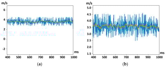
Figure 5.
(a) Output with random noise of magnitude ±1. (b) Output with random noise of magnitude ±2.
As shown in Figure 5a, with a single layer of extended Kalman filtering, the original base number constant 4 is shown in Figure 5b. The output result is different from the original base number 4, so it still causes errors from the original signal that must be compensated in the controller design. The gyro stabilization system designed by this institute is equipped with a three-gyro system on a drone and sacrifices one axis as a calibration axis for each unit of inertial measurement. The three inertial measurement outputs are complementary to the other two. Furthermore, the stability accuracy of drones and optoelectronic payloads are improved. The angular acceleration and acceleration output by the inertial measurement unit is obtained through an integrator, and the speed directly enters the adaptive extended Kalman filter loop. The angular velocity then outputs the angle data through the integrator and into the adaptive extended Kalman filter loop. The angular velocity and velocity output is integrated through the angular acceleration and acceleration output from the inertial measurement unit, and the angular velocity is output as an angle once integrated. The system designs a low-pass filter at the angular acceleration to filter and output to the trigger unit, where the unit decides to extend the Kalman filter filtering times. Through the final outputs of angle and speed to compare whether its Kalman gain value is much low, and raise a correction warning.
In the system design layout, the low-pass filter is generally limited to the average value of the input signal. The current average value of the input signal is obtained through the average filter, and upper and lower limits are given for the average value of the input signal. The process of Kalman filtering mainly avoids triggering more layers of extended Kalman filtering, so the limits for this low-pass filtering are shown in Table 2.
Table 2.
Design logic of upper-limit modulation of low-pass filter before trigger.
When the difference is larger, a multi-layer Kalman filter is used. Due to the infinite increase in the simulation, the experimental hardware is physically limited in the actual environment. There must be an upper limit and a warning to provide a gyroscope for recalibration and a warning that the Kalman filter gain is too low and needs to be recalibrated. Among them, judgment is given in the experiment.
In the actual flight process of the strong wind environment or high-speed flight, the acceleration has a chance to exceed 6 m/s2, so only the alarm reminder is provided; when the square difference exceeds 8 m/s2, the damage to the aircraft is lost. Therefore, during the process of warning and calibration of the gyroscope, it is detected synchronously whether the inertial gauge is malfunctioning or other sensing element is malfunctioning.
Figure 6 shows the result with the analog input of the sine wave and with one layer EKF. The input signal source is blue, the output signal after filtering through EKF is orange, and the output image at the same time is 54 fps. The average power consumption of the body system is 5.233 W.
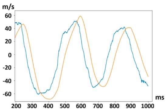
Figure 6.
Output response with EKF of 1 layer.
Figure 7 shows the result with the analog input of the sine wave and with the EKF of three layers. The input signal source is marked by a blue line, and the output signal with filtering through EKF is as an orange line. The frame rate of the output image is 41 fps. The average power consumption of the body system is 7.006 W.
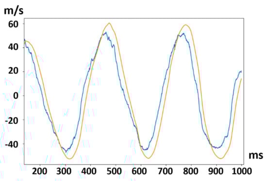
Figure 7.
Output response with EKF of 3 layers.
Figure 8 shows the result with the analog input of a sine wave and with an EKF of four layers. The input signal source is a blue line, and the output signal is an orange line. The output frame rate is 39 fps. The average power consumption of the body system is 7.853 W.
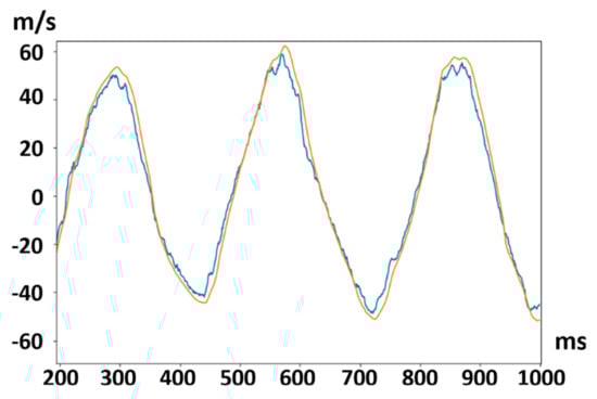
Figure 8.
Output response with EKF of 4 layers.
Figure 9 shows the result with the analog input of a straight-up and EKF of one layer. The input signal source is a blue line, and the output signal with EKF is an orange line. The output image is 54 fps per frame, while the average power consumption of the body system is 4.321 W.
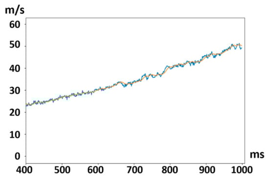
Figure 9.
Output response with EKF of level 1.
Figure 10 shows the result with three layers of EKF. The input signal source is a blue line, and the output signal is an orange line. The output image at the same time is 43 fps, and the average power consumption of the body system is 6.337 W.
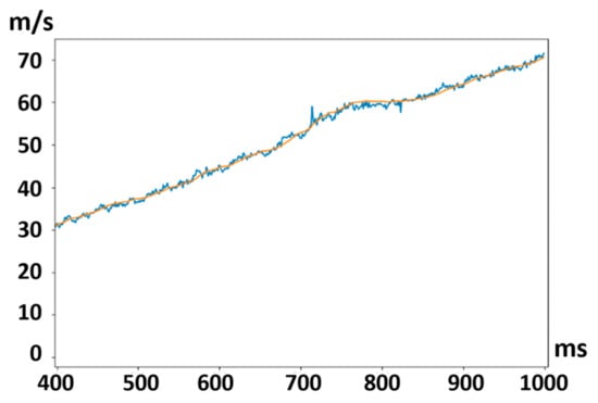
Figure 10.
Output response with EKF of level 3.
Figure 11 shows the result with the analog input of a straight-up and EKF of four layers. The input signal source is a marked blue line, and the output signal is a marked orange line. The output frame rate is 40 fps, and the average power consumption of the body system can be calculated as 7.100 W.
Figure 11.
Output response with EKF of level 4.
After adaptive multi-layer extended Kalman filtering, the output information can be provided to the image compensation for the stabilization effect that cannot be achieved by mechanical stabilization. As shown in Figure 12, the image vibration compensation is provided after filtering through the gyroscope to fit the image stabilization requirements of the drone or photoelectric payload
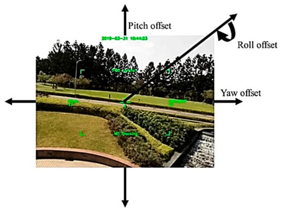
Figure 12.
Image vibration compensation with filtering through the gyroscope.
The angle of view of the roll effect when the drone is placed horizontally is shown in Figure 13a, and the angle of view of the payload tilted by 45 degrees is shown in Figure 13b. The image can be compensated by the gyroscope to achieve the effect of non-mechanical stabilization.
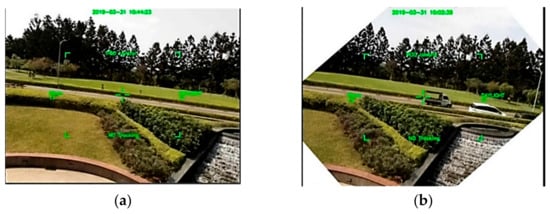
Figure 13.
(a) Perspective of Payload Level (b) Payload angle of 45°.
Figure 14 shows the result of a single-layer EKF actually swinging within degrees. The input signal is blue, and the output signal is orange. The output image is 56 fps, airborne. The average power consumption of the ROS hardware system is 4.511 W.
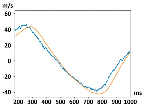
Figure 14.
Output response of single-layer EKF with actually swaying within degrees.
Figure 15 shows the result of two layers of EKF flying in the range of degrees. The input signal is blue, the output signal is orange, and the output image is 49 fps. The average power consumption of the ROS hardware system is 5.277 W.
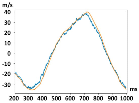
Figure 15.
Output response of 2 layers EKF with actually swaying within degrees.
Figure 16 shows the result of three layers EKF under actually swinging within degrees. The input signal is blue, the output signal is orange, and the output image is 43 fps. The average power consumption is 6.866 W.
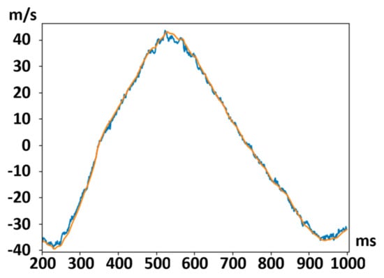
Figure 16.
Output response of 3 layers EKF with actually swaying within degrees.
Figure 17 shows the result of four layers of EKF with actually swinging at degrees. The input signal is blue, and the output signal is orange. The output image is 38 fps. The average power consumption of the ROS hardware system is 7.122 W.
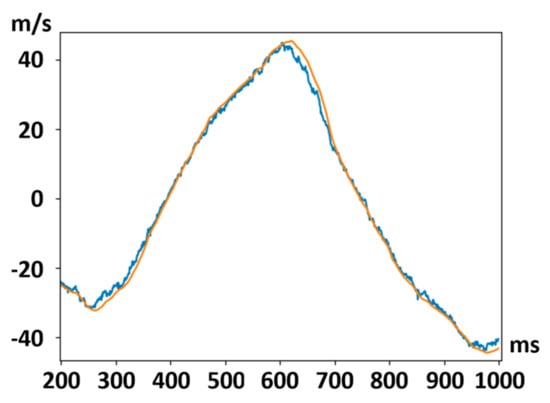
Figure 17.
Output response of 3 layers EKF with actually swaying within plus or minus 40 degrees.
Figure 18 shows the result of a single-layer EKF actually swinging within degrees. The input signal is blue, and the output signal is orange. The output image is 51 fps. The average power consumption of the ROS hardware system is 3.998 W.
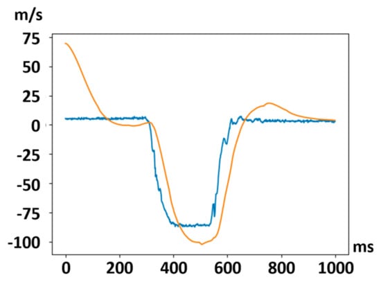
Figure 18.
Output response of single-layer EKF with actually swaying within degrees.
Figure 19 shows the result of a single-layer EKF actually swinging within degrees. The input signal is blue, and the output signal is orange. The output image at the same time is 38 fps. The average power consumption of the ROS hardware system is 5.512 W.
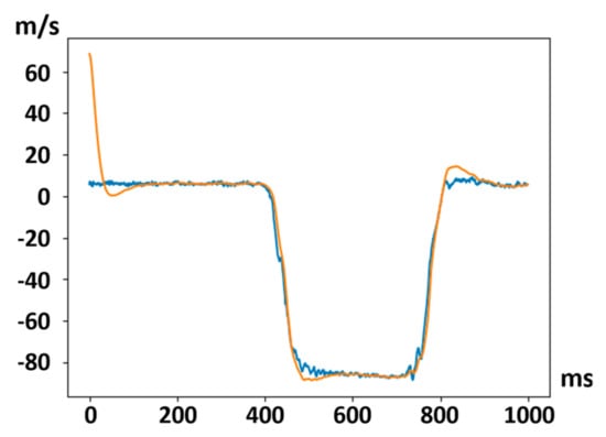
Figure 19.
Output response of adaptive multi-layer EKF with actually flying within degrees.
In the above verification data, it can be found that the method designed in this study is feasible. Despite the constraints of the hardware, the simultaneous processing of image and gyro information by a single processor results in a reduction in frames per second and cannot maintain the original image output of 60 fps. Table 3 shows the comparison between the proposed method and the traditional method that separates frame stabilization and image stabilization. Note that the gimbal holder is locked and can be measured during the study. It can be seen that using the traditional method, because the camera is separated from the gimbal frame, the frame rate of the output image is corrected and stabilized by the fixed global image of each frame, so it is kept at 50 fps. However, the proposed method in this study uses a single GPU for calculation, provides partial sampling and performs adaptive Kalman filtering for image stabilization, and cannot provide stable output frames per second, which is between 31 and 56 fps. In the power consumption comparison of GPU, the average power consumption of the traditional method is 9.6 watts, and the power consumption of the method designed in this study is 6.3 watts. In the comparison of the horizontal and vertical angles with the maximum allowable and no steady-state error, because the traditional method uses global image sampling, the cropping area is small, and the sampling cannot exceed the existing steady-state error, so the horizontal angle cannot be shifted by more than degrees, and the vertical cannot exceed degrees. The method used in this study is local sampling, so as long as it is within the camera’s viewing angle, it can be sampled and corrected at the same time with the gyroscope. Therefore, the horizontal angle cannot be offset by more than degrees, and the vertical angle cannot exceed degrees.
Table 3.
Comparison table between the traditional method without motor drive and the method used in this study.
However, in terms of practical application scenarios, the ring frame design of the traditional optoelectronic payload will activate the motor for hardware stabilization, thus increasing the maximum horizontal and vertical allowable angles, as shown in Table 4. Horizontal and vertical angles can be rotated without restriction. However, in this way, the power consumption is greatly increased to 32.1 watts.
Table 4.
Comparison table between the traditional method with motor drive and the method used in this study.
4. Conclusions
According to the experimental results, the processing time of the proposed method in the same hardware, fault limit, and camera field of view was compared with traditional frame correction and full image stabilization methods. The design method of this study is more effective than the traditional method in the efficient application of image resources. However, according to the comparison, the field of view in this research method is limited by the viewing angle of the camera. The special feature of this method is that it does not require the use of a motor for stabilization. Therefore, as drones shrink in size, there is less need for energy usage. For future applications, multiple aperture cameras will be used for panoramic shooting without dead angle, and image stabilization will be performed at the same time. This has actually been used in a few advanced anti-radar manned aircraft in the world at present, and the purpose is to reduce the radar reflection area of the external pod.
Therefore, based on this research, when more aperture cameras are used for image stabilization, resources can be more effectively used for calculation, and the image delay and power consumption can be reduced.
Author Contributions
Conceptualization, C.-Y.L. and W.-S.Y.; methodology, C.-Y.L. and W.-S.Y.; software, C.-Y.L.; validation, C.-Y.L.; formal analysis, C.-Y.L. and W.-S.Y.; investigation, C.-Y.L. and W.-S.Y.; resources, C.-Y.L.; data curation, C.-Y.L.; writing—original draft preparation, C.-Y.L.; writing—review and editing, W.-S.Y.; visualization, C.-Y.L. and W.-S.Y.; supervision, W.-S.Y. All authors have read and agreed to the published version of the manuscript.
Funding
This research was funded by Ministry of Science and Technology (Taiwan), grant number MOST 110-2221-E-992-064-.
Conflicts of Interest
The authors declare no conflict of interest.
References
- Wang, D.; Zhang, H.; Ge, B. Adaptive Unscented Kalman Filter for Target Tacking with Time-Varying Noise Covariance Based on Multi-Sensor Information Fusion. Sensors 2021, 21, 5808. [Google Scholar] [CrossRef] [PubMed]
- Mokbel, H.F.; Ying, L.Q.; Roshdy, A.A.; Hua, C.G. Design optimization of the inner gimbal for dual axis inertially stabilized platform using finite element modal analysis. Int. J. Mod. Eng. Res. 2012, 2, 239–244. [Google Scholar]
- Brake, N.J. Control System Development for Small UAV Gimbal. Ph.D. Thesis, California Polytechnic State University, San Luis Obispo, CA, USA, 2012. [Google Scholar]
- Qadir, A.; Neubert, J.; Semke, W. On-board visual tracking with unmanned aircraft system (uas). In AIAA Infotech@ Aerospace; American Institute of Aeronautics and Astronautics: St. Louis, MO, USA, 2011. [Google Scholar]
- Li, W.; Ren, S.Q.; Zhao, H.B. Influence of three-axis turntable error on gyro calibration accuracy. Electr. Mach. Control 2011, 15, 101–106. [Google Scholar]
- Bolme, D.S.; Beveridge, J.R.; Draper, B.A.; Lui, Y.M. Visual object tracking using adaptive correlation filters. In Proceedings of the 2010 IEEE Computer Society Conference on Computer Vision and Pattern Recognition, San Francisco, CA, USA, 13–18 June 2010. [Google Scholar]
- Alex, K.; Sutskever, I.; Hinton, G.E. ImageNet classification with deep convolutional neural networks. Commun. ACM 2017, 60, 84–90. [Google Scholar]
- Wang, Y.; Mu, X. Dynamic siamese network with adaptive Kalman filter for object tracking in complex scenes. IEEE Access 2020, 8, 222918–222930. [Google Scholar] [CrossRef]
- Zhang, T.; Shen, D.; Liu, C.; Xu, H. “A Novel Iterative Learning Control Approach Based on Steady-State Kalman Filtering”, special section on design and analysis techniques in iterative learning control. Digit. Object Identifier 2019, 7, 99371–99380. [Google Scholar]
- Liu, C.; Shui, P.; Wei, G.; Li, S. Modified unscented Kalman filter using modified filter gain and variance scale factor for highly maneuvering target tracking. J. Syst. Eng. Electron. 2014, 25, 380–385. [Google Scholar] [CrossRef]
- Zhang, X.; He, B.; Li, G.; Mu, X.; Zhou, Y.; Mang, T. Navnet: AUV Navigation Through Deep Sequential Learning. Digit. Object Identifier 2020, 8, 59845–59861. [Google Scholar] [CrossRef]
- Zhou, S.; Shen, C.-Y.; Zhang, L.; Liu, N.-W.; He, T.-B.; Yu, B.-L.; Li, J.-S. Dual-optimized adaptive Kalman filtering algorithm based on BP neural network and variance compensation for laser absorption spectroscopy. Opt. Express 2019, 27, 31874–31888. [Google Scholar] [CrossRef] [PubMed]
- Chabuda, A.; Durka, P.; Zygierewicz, J. High frequency SSVEP-BCI with hard ware stimuli control and phase-synchronized comb filter. IEEE Trans. Neural Syst. Rehabil. Eng. 2018, 26, 344–352. [Google Scholar] [CrossRef] [PubMed]
- Li, C.; Shao, L.; Jiang, L.; Qiu, X.; Wei, J.; Ma, W. Simultaneous measurements of CO and CO2 employing wavelength modulation spectroscopy using a signal averaging technique at 1.578 μm. Appl. Spectrosc. 2018, 72, 1380–1387. [Google Scholar] [CrossRef] [PubMed]
- Zanni, L.; Boudec, J.Y.L.; Cherkaoui, R.; Paolone, M. A prediction-error covariance estimator for adaptive Kalman filtering in step-varying processes: Application to power-system state estimation. IEEE Trans. Contr. Syst. Technol. 2017, 25, 1683–1697. [Google Scholar] [CrossRef] [Green Version]
- Fan, X.; Wang, J.; Zhu, D.; Qi, T. Speckle noise reduction technique for lidar echo signal based on self-adaptive pulse-matching independent component analysis. Opt. Laser. Eng. 2018, 103, 92–99. [Google Scholar]
- Zhang, J.; Zhou, W.; Wang, X. UAV Swarm Navigation Using Dynamic Adaptive Kalman Filter and Network Navigation. Sensors 2021, 21, 5374. [Google Scholar] [CrossRef]
- Yazdkhasti, S.; Sasiadek, J.Z. Multi Sensor Fusion Based on Adaptive Kalman Filtering. In Advances in Aerospace Guidance, Navigation and Control; Springer: Berlin/Heidelberg, Germany, 2018; pp. 317–333. [Google Scholar]
Publisher’s Note: MDPI stays neutral with regard to jurisdictional claims in published maps and institutional affiliations. |
© 2022 by the authors. Licensee MDPI, Basel, Switzerland. This article is an open access article distributed under the terms and conditions of the Creative Commons Attribution (CC BY) license (https://creativecommons.org/licenses/by/4.0/).