Genetic Algorithm for the Optimization of a Building Power Consumption Prediction Model

Abstract

Accurately predicting power consumption is essential to ensure a safe power supply. Various technologies have been studied to predict power consumption, but the prediction of power consumption using deep learning models has been quite successful. However, in order to predict power consumption by utilizing deep learning models, it is necessary to find an appropriate set of hyper-parameters. This introduces the problem of complexity and wide search areas. The power consumption field should be accurately predicted in various distributed areas. To this end, a customized consumption prediction deep learning model is needed, which is essential for optimizing the hyper-parameters that are suitable for the environment. However, typical deep learning model users lack the knowledge needed to find the optimal values of parameters. To solve this problem, we propose a method for finding the optimal values of parameters for learning. In addition, the layer parameters of deep learning models are optimized by applying genetic algorithms. In this paper, we propose a hyper-parameter optimization method that solves the time and cost problems that depend on existing methods or experiences. We derive a hyper-parameter optimization plan that solves the existing method or experience-dependent time and cost problems. As a result, the RNN model achieved a 30% and 21% better mean squared error and mean absolute error, respectively, than did the arbitrary deep learning model, and the LSTM model was able to achieve 9% and 5% higher performance.

1. Introduction

In many countries, power consumption is increasing due to rapid economic growth and population growth [1]. Electrical energy is consumed in tandem with its production due to its physical characteristics, so the accurate prediction of power demand is extremely important for a stable power supply. For accurate power demand, power consumption is predicted through AMI and IoT sensors in cities, buildings and furniture. Recently, ICT technology has been extensively applied to the energy field, and smart grids (intelligent power grids) that use energy efficiently are being implemented [2,3]. This means that a new electricity consumption ecosystem is being created, and at its center is the smart grid. It is time for efficient power management in society as a whole to achieve carbon neutrality. To this end, it is necessary to fuse ICT technology to predict power consumption more accurately, efficiently, and according to patterns. Various technologies are being studied to predict power consumption. Previously, time series and prediction models were generally used [4]. ARIMA-based models [5], statistical models using single time series data or multivariate linear regression models using multivariate data related to power demand have generally been used to predict consumption. However, predictions by nonlinear models are more efficient than linear models. Machine learning and deep learning models are generalized nonlinear predictions, and their frequency of use in power demand prediction research has been increasing [5,6]. The structure of deep learning models is divided into an input layer, a hidden layer and an output layer by statistical learning algorithms. Each layer has a weight and allows the resulting value to be approximated to the actual value according to the weight. The structure of this deep learning model is determined by a number of hyper-parameters. The model must have an appropriate structure to ensure optimal performance. However, the optimal hyper-parameter value is irregular and highly influenced by the user’s experience [7]. There is also a very large search space for finding the optimal structure. To this end, it is necessary for researchers to design many deep learning models, or optimal values can be derived with high time and monetary costs [8]. There are traditional methods for random search and grid search, but the risk of falling into local optima is high. Genetic algorithms are methodologies described in Darwin’s theory of evolution [9,10]. The objective is to derive excellent genes through genetic mechanisms and natural selection. In order to find the optimal solution to complex algorithms through natural evolution, it is appropriate to find the optimal solution using genetic algorithms. Deriving the optimal hyper-parameter value of deep learning models using genetic algorithms is a lightweight procedure that can achieve appropriate performance without requiring expertise or high time and cost consumption. In this study, the optimal hyper-parameter values of the deep learning model were derived using the genetic algorithm to obtain higher performance than the deep learning model depending on the user’s empirical evidence. The proposed method also obtained higher performance than a random search. It was confirmed that deriving the optimal hyper-parameter value of the deep learning model using genetic algorithms can enable appropriate performance without requiring expertise or high time and cost consumption. The composition of this paper is as follows. Section 2 looks at existing methods for predicting power consumption and optimizing prediction models. Section 3 proposes a method for optimizing power consumption prediction models. Section 4 compares the performance of the proposed method. Finally, Section 5 presents the conclusions of this study.

2. Related Works

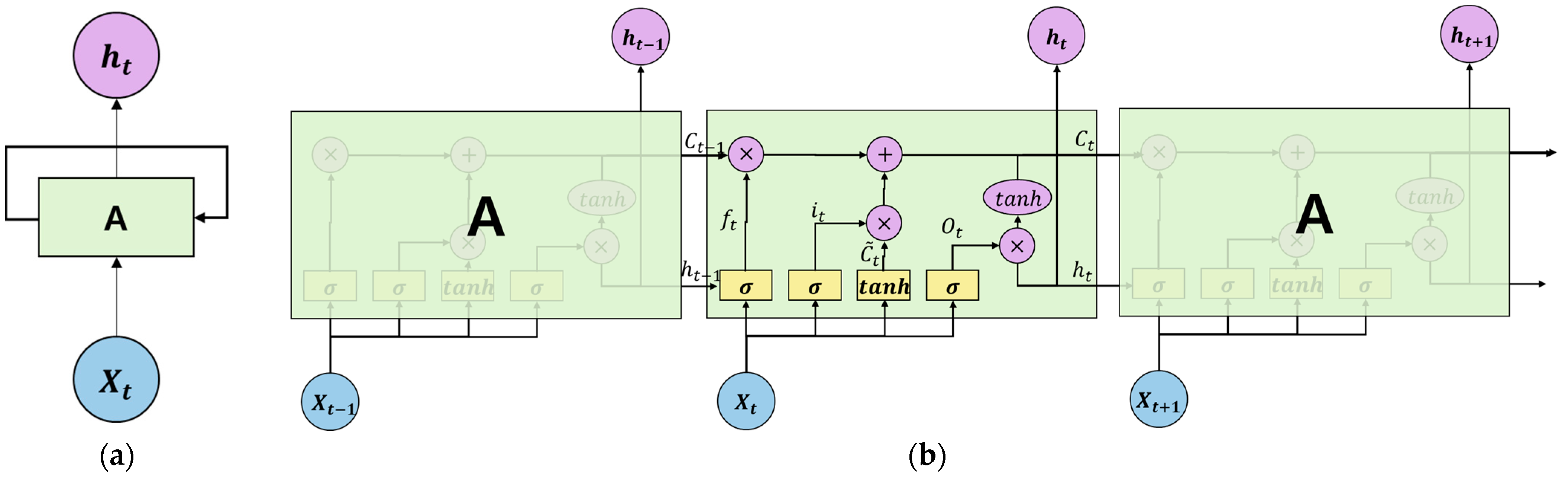
2.1. Deep Learning Model

In recent years, many researchers have investigated various algorithms for predicting actual power demand. The deep learning model, called the artificial neural network, includes a forward neural network and a backpropagation neural network consisting of nonlinear functions, such as activation functions [11,12]. These deep learning models are used in various ways, such as Convolutional, Recurrent and Reinforcement models, according to the characteristics of the data and the domains. Power consumption prediction is being developed mainly with Recurrent Neural Networks (RNNs) [13].

The RNN is a cyclic neural network that is linked to the next hidden layer of the neural network according to time, and it is a model that considers the impact of previous samples on the next sample [14]. Because the prediction of power consumption determines the future according to seasonality and time, this paper uses a one-way RNN structure. RNN models can obtain power demand values that determine and predict whether historical data affect previous data according to the weight ${\mathrm{W}}_{\mathrm{h}}$ between weights ${\mathrm{W}}_1$, ${\mathrm{W}}_2$ and neural networks, as shown in Figure 1.

Long Short-Term Memory (LSTM) is a neural network that compensates for the shortcomings that existing RNN models have, including difficulty remembering information that is far from the predicted values [15]. The LSTM model layer consists of five structures: the Cell State, Forget Gate, Input Gate, Cell State Update and Output Gate. The equation for each module is as follows. Figure 1b shows a simple LSTM structure. The portion to which each of the four equations is applied inside LSTM can be identified.

$$f_t=\sigma \left(W_f·\left[h_{t-1}, x_t\right]+b_f\right)$$

(1)

$$i_t=\sigma \left(W_t·\left[h_{t-1}, x_t\right]+b_i\right), \widetilde{C_t}=\tan \mathrm{h}(W_C·\lceil h_{t-1}, x_t\rceil +b_c$$

(2)

$$C_t=f_t\ast C_{t-1}+i_t\ast {\tilde{C}}_t$$

(3)

$${\mathrm{o}}_{\mathrm{t}}=\sigma \left(W_o\left[h_{t-1}, x_t\right]+b_o\right),{\mathrm{h}}_{\mathrm{t}}=o_t\ast \tan \mathrm{h}\left(C_t\right)$$

(4)

2.2. Hyper-Parameters of Deep Learning

As mentioned in the previous section, the deep learning model has parameters for optimization, such as various layers and activation functions. Hyper-parameters can change the performance of the model and prevent over-fitting or under-fitting. Activation functions can be used to introduce nonlinearity, especially in algorithms. At first, nonlinearity was introduced through the tan h activation function, and many deep learning models were developed with the advent of the Rectified Linear Unit (ReLU). However, the ReLU activation function treats all negative numbers as zero. Activation functions Leaky RELU and ELU have also been introduced and are used to activate negative numbers [16,17]. The two activation functions are utilized by multiplying a small parameter (a, alpha value) or 0.1 without treating negative values as zero. In addition, the optimization algorithm for optimizing the model is an algorithm for reducing the loss of the model. It is generally called Gradient Descent (GD). However, GD’s optimization problem is that it requires a lot of time. Stochastic Gradient Descent (SGD) has generally been used to solve this problem. SGD allows faster convergence by randomly selecting data samples and calculating the slope for one sample [18]. Based on SGD, the ADAM optimization function can appropriately select the step size and optimization direction for optimization by estimating the mean and variance values [19]. ADAMAX is an algorithm extended to ${\mathrm{L}}_{\mathrm{p}}$ Norm from a method for optimizing the learning rate based on the ${\mathrm{L}}_2$ Norm of the ADAM optimization function [20]. Thus, for deep learning, there are various hyper-parameters that must be generalized by preventing over-fitting and under-fitting, such as learning rate and dropout, as well as various activation functions and optimization functions.

2.3. Neural Architecture Search

NAS stands for Neural Architecture Search and is a research field that has emerged with deep learning models [21]. Deep-learning-based models also need to have a network structure in order to achieve appropriate performance according to the given data or a domain. More specifically, the NAS automatically designs the structure of the network model. Quickly finding a network structure that can optimize the performance of the model through NAS can reduce the time and cost of the training process. To optimize the network model structure, measures such as reinforcement learning and Bayesian optimization, as well as random search and grid search, are used. However, these methods consume a lot of time [22,23]. NAS may need to design a layer structure in a complex area, but it can also adjust the number of units in a fixed layer to derive lightweight and optimal performance with an appropriate number of parameters.

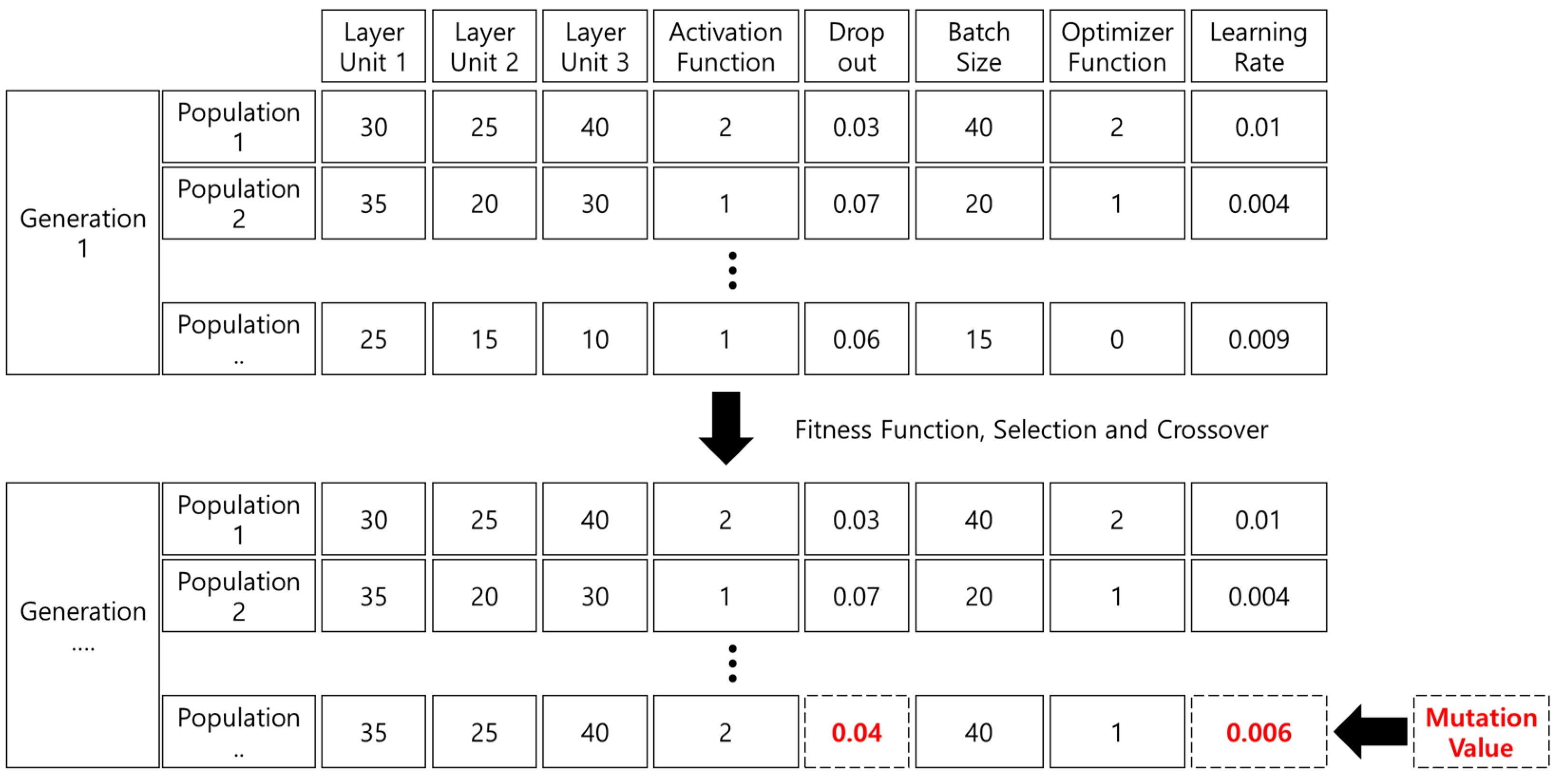
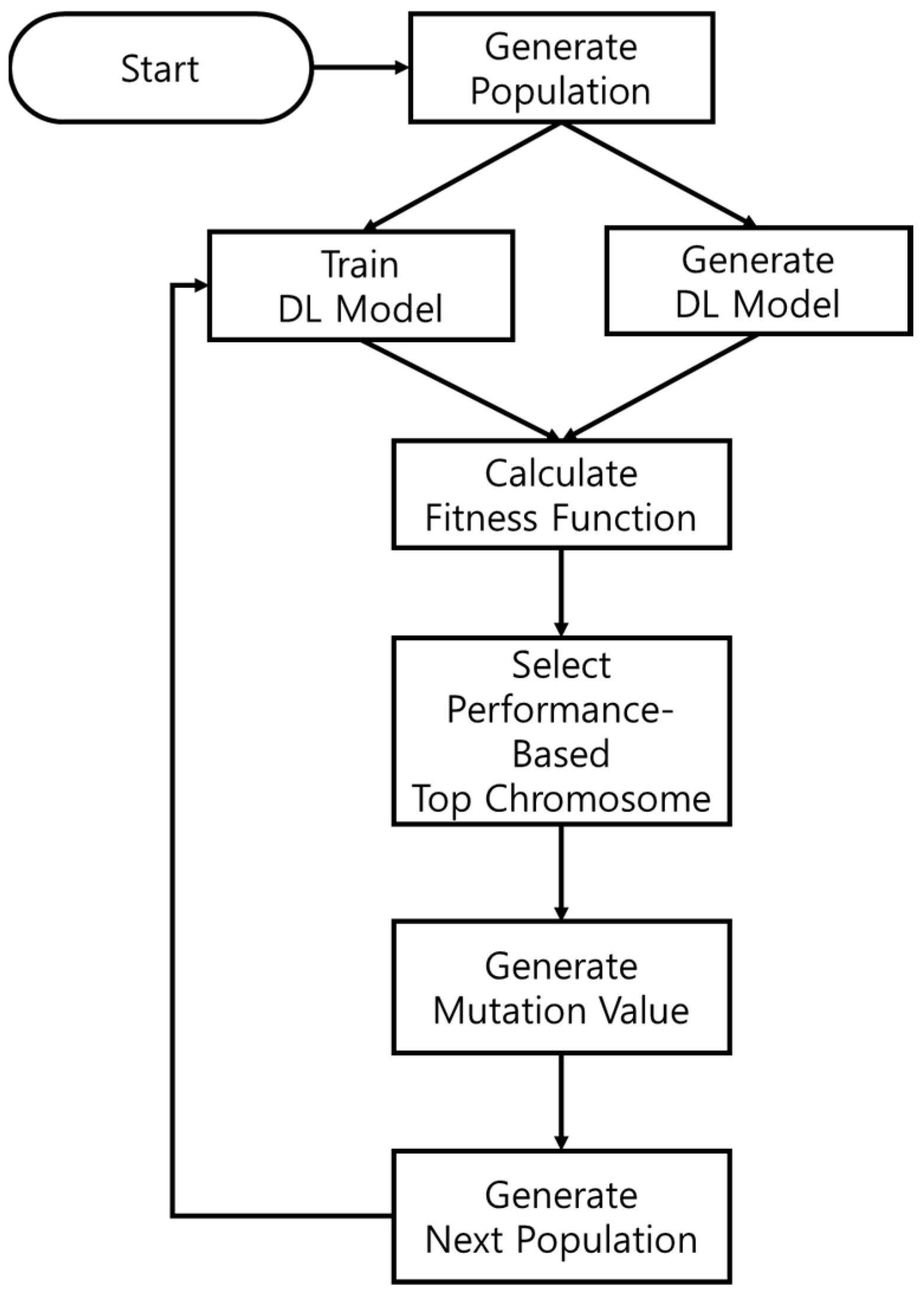
2.4. Genetic Algorithm

Research using machine learning techniques or genetic algorithms to accurately predict existing power demand continues. Genetic algorithms derive effectiveness from various optimization problems [9,10,24,25,26]. Genetic algorithms use populations of multiple potential solutions to navigate, transfer excellent solutions to the next generation, and thus converge on global solutions. The theory of genetic algorithms is easy to use, and the search for optimal solutions is excellent. Therefore, the advantage is that it can be applied in various ways to optimization problems and can effectively be applied to problems with large search spaces or many constraints.

The genetic algorithm is generally composed of four parts: generation, population, mutation and crossover. Each generation consists of a population capable of solving problems. Parent chromosomes list the best genes that satisfy the fitness function among the genes that make up the population. The evaluation function is used to measure the performance and fit of the chromosomes. Excellent genes are selected using an evaluation function. The next generation is created by crossing over the best genes. This allows only the best chromosomes to remain and satisfies the evaluation function as generations pass. However, because the algorithm can fall into regional optimization, it generates a mutation to derive the global optimization. Thus, one of the characteristics of genetic algorithms is not to limit a single chromosome to a search space, but to have a large search space, called a population of many chromosomes, which reduces the probability of falling into a regional solution. The number of chromosomes constituting the generation may be variously configured according to an optimization problem.

2.5. Genetic-Algorithm-Based Optimal Model

The genetic-algorithm-based optimal model not only optimizes learning parameters using genetic algorithms, but it also optimizes the structural parameters of deep learning models. Models optimized using genetic algorithms generally achieve higher performance by automatically optimizing model structure parameters without investing much time or cost based on user experience. Through this process, the optimal model for data characteristics is generated, rather than comparing deep learning models with different parameter counts with each other and comparing the overall layer model structure.

3. Deep Learning Network and Hyper-Parameter Optimization

3.1. Genetic Algorithm for the Deep Learning Model

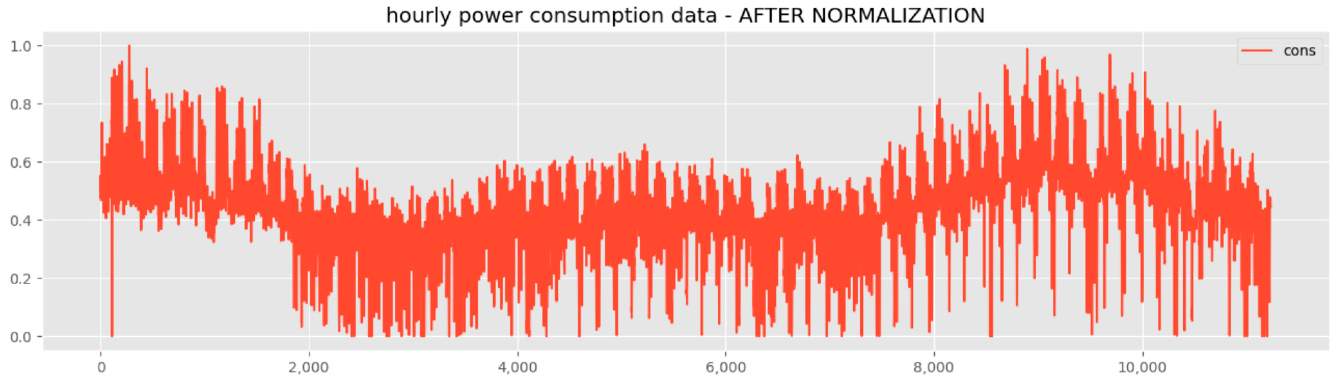
The network architecture of the deep learning model for power consumption prediction, as well as the genetic algorithm structure for hyper-parameter optimization, are shown in Figure 2. The network architecture and hyper-parameter coefficients according to the flowchart are determined as shown in Figure 3. The genetic algorithm proposed in this paper allows us to find not only the learning coefficient but also the optimal value of the layer coefficient of the deep learning model. We initialize the first generation for the optimization of network structure and hyper-parameter optimization through genetic algorithms. One generation consists of the number of units in the layer, the activation function (RNN Model), the optimization function, the batch size, the dropout coefficient and the learning rate. For hybridization, the performance is measured using an evaluation function, and a new gene is generated by crossbreeding the higher genes. The genetic makeup of the exact RNN model is shown in

Table 1. RNN gene: hyper-parameters.

Gene	Min		Max
Layer 1 Unit	20		50
Layer 2 Unit	20		50
Layer 3 Unit	20		50
Activation Function	tan h	Leaky ReLU		ELU
Optimizer	SGD	ADAM		ADAMAX
Dropout	0.01		0.2
Batch size	20		50
Learning Rate	0.001		0.015

, and the genetic makeup of the LSTM model is shown in

Table 2. LSTM gene: hyper-parameters.

Gene	Min		Max
Layer 1 Unit	20		50
Layer 2 Unit	20		50
Layer 3 Unit	20		50
Optimizer	SGD	ADAM		ADAMAX
Dropout	0.01		0.2
Batch size	20		50
Learning Rate	0.001		0.015

.

To quickly find the optimal global solution for the genetic algorithm, the number of Epochs was designated as five. After learning five times, a test dataset was utilized to compare the mean squared error (MSE) performance; therefore, the best chromosome could be selected. A new generation was created by selecting an upper chromosome and hybridizing the two upper chromosomes at an arbitrary ratio. After generating a new generation by selecting a higher chromosome, a mutation value was added to at least one randomly designated chromosome. The range of mutant chromosome values for applying mutant chromosomes to new generations is shown as follows in

Table 3. Mutation values.

Gene	Min	Max
Layer 1 Unit	−10	10
Layer 2 Unit	−10	10
Layer 3 Unit	−10	10
Activation Function	Random
Optimizer	Random
Dropout	−0.1	0.1
Batch Size	100	200
Learning Rate	−0.1	0.1

.

A mutated chromosome applies a random value between the minimum and maximum values expressed in Table 3 to the new chromosome to generate the next generation to which the mutation is applied.

3.2. Dataset

In this study, the data used in the deep learning model for optimizing the actual power consumption prediction were the power consumption data of the construction of Building No. 7 at Chonnam National University. The data consisted of 11,232 data points collected on an hourly basis over a total of 468 days from 1 January 2021 to 13 April 2022.

Figure 4 shows the normalized data. In order to utilize actual power data, outliers were not removed or used. In order to use the power consumption data for deep learning, the window size was designated and configured; therefore, the power consumption could be predicted by viewing the window size. To this end, the window size was designated as 20. For the generalization of the general deep learning model, the dataset was classified as 80% training data and 20% testing data. The dataset configuration was approximately as shown in

Table 4. Configuring the dataset used for training.

Training Dataset		Test Dataset
Input	Target	Input	Target
(8985, 20, 1)	(8985, 1)	(2227, 20, 1)	(2227, 1)

. The power consumption data consisted of a minimum of 0 kWh to a maximum of 297.49 kWh. This introduced a problem in which a long time was required during the optimization process when learning with the deep learning model, or there may have been bias toward changes in some values. To prevent this, the data were normalized to the training dataset and applied to the testing dataset.

4. Results and Discussion

4.1. Experimental Setting

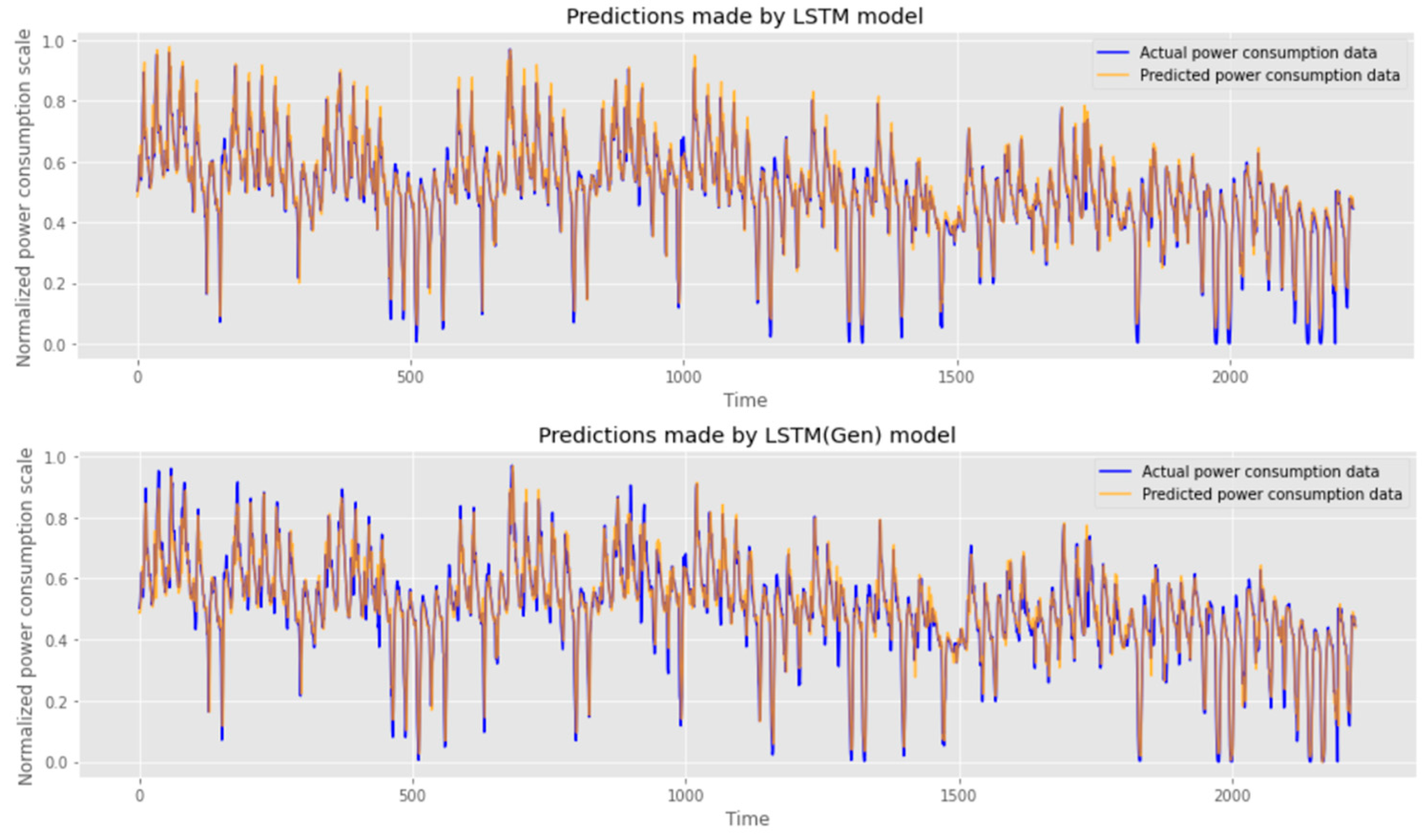
Neural networks were created to implement the method proposed in this study using Python and Keras bases. This learning environment has been studied using high-performance servers that support the Intel i9 X-series CPU, 128 GB RAM, Ubuntu 18.04 and the NVIDIA RTX 3090 GPU. A total of 50 generations of genetic algorithms were computed, and the parent chromosome for hybridization was set to five genes. The evaluation function compared the performance of the chromosomes using the MSE. For the performance comparison, the learning parameters of the existing RNN model, LSTM model, genetic-algorithm-based RNN, LSTM model and random-search-based RNN model are shown in

Table 5. Performance comparison of existing deep learning models and optimized deep learning models.

Gene	RNN	Random-Search-Based RNN	Genetic-Based RNN Model	LSTM	Genetic-Based LSTM Model
Layer 1 Unit	40	44	42	40	50
Layer 2 Unit	40	47	59	40	20
Layer 3 Unit	40	35	29	40	31
Activation Function	tan h	Leaky RELU	ELU	-	-
Optimizer	ADAM	ADAM	ADAM	ADAM	ADAM
Dropout	0.15	0.08	0.02	0.15	0.04
Batch Size	10	28	40	10	20
Learning Rate	0.01	0.002	0.008	0.01	0.004

. As shown in Table 5, the RNN model sets the layer unit to 40, the activation function to tan h, the optimizer to ADAM, the dropout to 0.15, the batch size to 10 and the learning rate to 0.01. The LSTM model was set in the same way, except for the active function. As a result, the optimizer for both random search and the proposed method derived the ADAM function. The hyper-parameters derived by the random search method and the proposed method were generally large for layer units 1 and 2, and they were small for layer 3 unit. In the LSTM model, the derived layer 2 unit was small. The dropout was smaller than that of the heuristic model, and the batch size was large. The learning rate was very small compared to that of the previous one. It can be seen that the biggest difference was in the active function, batch size and learning rate.

Table 6. Comparison of generational time required between the proposed method and the random search method.

	Random-Search-Based Method	Proposed Method
Generation 1	668	704
Generation 2	666	683
Generation 3	662	612
Generation 4	665	602
Generation 5	664	598
Average running time	665	639.8

compares the time required for the proposed method and that of the the random search method in this paper. The values in the table are the time taken to learn 10 genes consisting of parameters in 5 Epochs. Random search took an average of 665 s to learn each generation, and the proposed method took 704 s in the first generation. However, it was confirmed that the average generation time was less than that of the random search method. We found that the proposed method learns 4% faster on average than random-search-based methods.

4.2. Result

Figure 5 shows the average MSE values for each generation through a genetic algorithm. In the figure, it can be seen that the minimum value, maximum value and average value are low on average. Figure 6 and Figure 7 visualize the fitness value derived when 10 genes are applied over 50 generations to optimize hyper-parameters by applying our proposed algorithm to the RNN and LSTM models. Looking at the fitness value for each gene, it can be seen that the newly derived genes can be used to find the global optimal solution as well as the continuous optimization as the generations progress.

MSE and Mean Absolute Error (MAE) performance indicators were used to compare the performance of the optimal hyper-parameters in this paper. The formulas for MSE and MAE are as follows. The MSE and MAE performance indicators are the most popular error functions used to optimize deep learning models.

$$\mathrm{MSE}=\frac{1}{n}{{\displaystyle \sum }}_{i=1}^n{\left(\widehat{Y_i}-Y_i\right)}^2$$

(5)

$$\mathrm{MAE}=\frac{1}{n}{{\displaystyle \sum }}_{i=1}^n\left|\widehat{Y_i}-Y_i\right|$$

(6)

Table 7. Comparison of performances.

Performance Function	RNN	Random-Search-Based RNN	Genetic-Based RNN Model	LSTM	Genetic-Based LSTM Model
MSE	0.00421	0.00314	0.00298	0.00261	0.00239
MAE	0.04884	0.03955	0.03874	0.0348	0.033

compares the performance of a model optimized by the method proposed in this paper, an existing model and a random-search-based model. The optimized RNN model shows a 30% improvement in MSE and a 21% improvement in MAE compared with the existing RNN model. The optimized LSTM model shows a 9% improvement in performance based on MSE and 5% improved performance based on MAE. The MSE of the RNN model found through random search showed a difference of 5% and 3%. It can be seen that the method proposed in this paper finds the optimum hyper parameter.

In Figure 8 and Figure 9, the predicted values of the model are visualized. It can be seen that the LSTM model performs better by default than the RNN model and that the model learned using hyper-parameters derived from the proposed method makes accurate predictions.

5. Conclusions

In this paper, the goal was to optimize the network structure of RNN models and LSTM models for a given power consumption dataset using genetic algorithms, as well as for the learning environment. The method of optimizing the genetic-algorithm-based hyper-parameters proposed in this paper was designed based on experience and time by an expert with existing artificial intelligence model knowledge and power-related knowledge. However, by automating these problems through the method proposed in this paper, not only was the artificial intelligence model for power requirement prediction optimized, but the performance was also enhanced. By learning the power requirement data of the actual building, it was possible to optimize the MSE and MAE performance by up to 30% and by at least 5%. Based on the MSE and MAE performance evaluation functions, the heuristic RNN model had MSE and MAE performances of 0.00421 and 0.04884, whereas the random-search-based RNN model had MSE and MAE performances of 0.00314, 0.03955. However, the genetic-algorithm-based RNN model achieved the highest performance with 0.00298 and 0.03874. Based on the LSTM model, it also had the existing MSE and MAE performances of 0.00261 and 0.0348, and the genetic-algorithm-based LSTM model achieved the highest performance with 0.00239 and 0.033. It can be seen that our applied genetic algorithms found the appropriate hyper-parameters of the deep learning model for power consumption prediction. In addition, it was found that the proposed method could be optimized by including not only parameters for learning but also the hyper-parameters of the deep learning structures in the range of genetic algorithms. In addition, although genetic algorithms can be parallel processed, this paper did not utilize the advantages of parallel processing. In addition, there exists a problem in which the computational complexity increases according to the fitness function. In the future, studies that solve these problems or initial gene selection according to power patterns will remain to be conducted.

References

1. Hilty, L.M.; Coroama, V.; de Eicker, M.O.; Ruddy, T.F.; Müller, E. The Role of ICT in Energy Consumption and Energy Efficiency; Empa Swiss Federal Laboratories for Materials Testing and Research: St. Gallen, Switzerland, 2009. [Google Scholar]
2. Lange, S.; Pohl, J.; Santarius, T. Digitalization and energy consumption. Does ICT reduce energy demand? Ecol. Econ. 2020, 176, 106760. [Google Scholar] [CrossRef]
3. Tuballa, M.L.; Abundo, M.L. A review of the development of Smart Grid technologies. Renew. Sustain. Energy Rev. 2016, 59, 710–725. [Google Scholar] [CrossRef]
4. Deb, C.; Zhang, F.; Yang, J.; Lee, S.E.; Shah, K.W. A review on time series forecasting techniques for building energy consumption. Renew. Sustain. Energy Rev. 2017, 74, 902–924. [Google Scholar] [CrossRef]
5. Ozturk, S.; Ozturk, F. Forecasting Energy Consumption of Turkey by Arima Model. J. Asian Sci. Res. 2018, 8, 52–60. [Google Scholar] [CrossRef] [Green Version]
6. Mocanu, E.; Nguyen, P.H.; Gibescu, M.; Kling, W.L. Deep learning for estimating building energy consumption. Sustain. Energy Grids Netw. 2016, 6, 91–99. [Google Scholar] [CrossRef]
7. Yu, T.; Zhu, H. Hyper-parameter optimization: A review of algorithms and applications. arXiv 2020, arXiv:2003.05689. [Google Scholar]
8. Young, S.R.; Rose, D.C.; Karnowski, T.P.; Lim, S.-H.; Patton, R.M. Optimizing deep learning hyper-parameters through an evolutionary algorithm. In Proceedings of the Workshop on Machine Learning in High-Performance Computing Environments, Austin, TX, USA, 15–20 November 2015. [Google Scholar]
9. Whitley, D. A genetic algorithm tutorial. Stat. Comput. 1994, 4, 65–85. [Google Scholar] [CrossRef]
10. Hamdia, K.M.; Zhuang, X.; Rabczuk, T. An efficient optimization approach for designing machine learning models based on genetic algorithm. Neural Comput. Appl. 2021, 33, 1923–1933. [Google Scholar] [CrossRef]
11. Pouyanfar, S.; Sadiq, S.; Yan, Y.; Tian, H.; Tao, Y.; Reyes, M.P.; Shyu, M.-L.; Chen, S.-C.; Iyengar, S.S. A Survey on Deep Learning: Algorithms, Techniques, and Applications. ACM Comput. Surv. 2018, 51, 1–36. [Google Scholar] [CrossRef]
12. Alom, M.Z.; Taha, T.M.; Yakopcic, C.; Westberg, S.; Sidike, P.; Nasrin, M.S.; Hasan, M.; Van Essen, B.C.; Awwal, A.A.S.; Asari, V.K. A State-of-the-Art Survey on Deep Learning Theory and Architectures. Electronics 2019, 8, 292. [Google Scholar] [CrossRef] [Green Version]
13. Petneházi, G. Recurrent neural networks for time series forecasting. arXiv 2019, arXiv:1901.00069. [Google Scholar]
14. Hewamalage, H.; Bergmeir, C.; Bandara, K. Recurrent Neural Networks for Time Series Forecasting: Current status and future directions. arXiv 2019, arXiv:1909.00590. [Google Scholar] [CrossRef]
15. Hochreiter, S.; Schmidhuber, J. Long Short-Term Memory. Neural. Comput. 1997, 9, 1735–1780. [Google Scholar] [CrossRef] [PubMed]
16. Sadeghi, A.; Wang, G.; Giannakis, G.B. Deep Reinforcement Learning for Adaptive Caching in Hierarchical Content Delivery Networks. IEEE Trans. Cogn. Commun. Netw. 2019, 5, 1024–1033. [Google Scholar] [CrossRef] [Green Version]
17. Dubey, A.K.; Jain, V. Comparative Study of Convolution Neural Network’s ReLu and Leaky-ReLu Activation Functions. In Applications of Computing, Automation and Wireless Systems in Electrical Engineering; Springer: Singapore, 2019; pp. 873–880. [Google Scholar]
18. Halgamuge, M.N.; Daminda, E.; Nirmalathas, A. Best optimizer selection for predicting bushfire occurrences using deep learning. Nat. Hazards 2020, 103, 845–860. [Google Scholar] [CrossRef]
19. Kingma, D.; Ba, J. Adam: A method for stochastic optimization. arXiv 2014, arXiv:1412.6980. [Google Scholar]
20. Vani, S.; Madhusudhana Rao, T.V. An Experimental Approach towards the Performance Assessment of Various Optimizers on Convolutional Neural Network. In Proceedings of the 2019 3rd International Conference on Trends in Electronics and Informatics (ICOEI), Tirunelveli, India, 23–25 April 2019. [Google Scholar]
21. Elsken, T.; Metzen, J.H.; Hutter, F. Neural Architecture Search: A Survey. arXiv 2018, arXiv:1808.05377. [Google Scholar]
22. Zoph, B.; Le, Q.V. Neural architecture search with reinforcement learning. arXiv 2016, arXiv:1611.01578. [Google Scholar]
23. Wu, J.; Chen, X.-Y.; Zhang, H.; Xiong, L.-D.; Lei, H.; Deng, S.-H. Hyperparameter optimization for machine learning models based on Bayesian optimization. J. Electron. Sci. Technol. 2019, 17, 26–40. [Google Scholar]
24. Xiao, X.; Yan, M.; Basodi, S.; Ji, C.; Pan, Y. Efficient Hyperparameter Optimization in Deep Learning Using a Variable Length Genetic Algorithm. arXiv 2020, arXiv:cs.NE/2006.12703. [Google Scholar]
25. Folino, G.; Forestiero, A.; Spezzano, G. A Jxta Based Asynchronous Peer-to-Peer Implementation of Genetic Programming. J. Softw. 2006, 1, 12–23. [Google Scholar] [CrossRef]
26. Forestiero, A.; Papuzzo, G. Agents-Based Algorithm for a Distributed Information System in Internet of Things. IEEE Internet Things J. 2021, 8, 16548–16558. [Google Scholar] [CrossRef]
Figure 1. Structure of simple RNN and LSTM models: (a) RNN architecture; (b) LSTM architecture.
Electronics 11 03591 g001
Figure 2. Flowchart of optimal model generation based on genetic algorithms.
Electronics 11 03591 g002
Figure 3. Genetic-algorithm-based optimization process.
Electronics 11 03591 g003
Figure 4. Preprocessed power consumption data.
Electronics 11 03591 g004
Figure 5. Minimum, maximum and average values of the fitness function for each generation.
Electronics 11 03591 g005
Figure 6. Visualized evaluation functions for each generation: RNN model.
Electronics 11 03591 g006
Figure 7. Visualized evaluation functions for each generation: LSTM model.
Electronics 11 03591 g007
Figure 8. Comparison of performance between existing RNN model (top) and optimized RNN model (bottom).
Electronics 11 03591 g008
Figure 9. Comparison of performance between existing LSTM model (top) and optimized LSTM model (bottom).
Electronics 11 03591 g009