Article

Determination of Excitation Amplitude and Phase for Wide-Band Phased Array Antenna Based on Spherical Wave Expansion and Mode Filtering

School of Electronic Engineering, Xidian University, Xi’an 710071, China
*
Author to whom correspondence should be addressed.
Electronics 2022, 11(21), 3479; https://doi.org/10.3390/electronics11213479
Submission received: 14 September 2022 / Revised: 21 October 2022 / Accepted: 25 October 2022 / Published: 26 October 2022
(This article belongs to the Special Issue Wideband and Multiband Antennas for Wireless Applications)

Abstract

:
A new method for solving the excitation amplitude and phase of wide-band phased array antenna is presented, in which spherical wave expansion and mode filtering (SWEMF) techniques are applied for the first time. Different from the previous methods that are required of matrix inversion or optimization iteration, the proposed SWEMF method is a forward calculation process. Thus, the solution is unique, and the result is closer to the true value. On the other hand, the SWEMF method only needs the total radiated field data of the array antenna in a small angular domain to ensure that the operation is simple and efficient. The effectiveness of the SWEMF method is successfully verified by examples of low sidelobe planar and linear arrays. The mean square error of the excitation amplitude can reach −38.88 dB. The range of excitation amplitude error is 0.05 v, and the excitation phase error is within 5.2°. This method takes about 60 s to calculate amplitude and phase at any one time. The feed amplitude and phase can be only calculated with the data in a small angular domain, and when the amount of data is small.

1. Introduction

Compared with a single antenna, the antenna array composed of multiple antenna elements can easily meet design requirements by adjusting the value of excitation amplitude, excitation phase, array elements, etc. [1,2]. If the antenna radiating element is incorrectly excited, it will affect the antenna radiation pattern, beam direction, sidelobe level, etc. [3,4]. At this current time, the phased array antenna cannot reach the optimal index of the required design. The antenna pattern will be deformed, which will cause the antenna to not work properly. As such, monitoring the excitation of the phased array antenna radiating element is a problem worthy of discussion.
Calculating phased array antenna excitation from external data is simple and efficient. L. Gattoufi, et al. [5] proposed a method to calculate the excitation of phased array elements through near-field measurement [6,7] data using the matrix method. However, the error produced is large when the short distance measurement is performed. J. A. Lord et al. [8] proposed a method to reconstruct the array antenna excitation from the measured near-field data using the phase inversion method. This method iteratively converges when the RMS magnitude and phase change, between the present output and previous output, fall below certain acceptable values. However, the inverse problem in these two methods may be ill-conditioned. This is because numerical errors are generated when inverting the interaction matrix.
Far-field measurement [9] can also play a role in inverting the excitation of radiating elements. Further, the rotating vector method [10] is a common method to calculate the feed of the antenna element. This method needs to measure far-field data under different phase shifter states. When the number of phase shifters is M and the number of units is N, 2M*N, measurements are required, which is a complex process for large arrays. A phase-shift measurement method can be combined with the coding matrix [11] in order to calculate the radiation element excitation. This method requires multiple measurements of the complete far-field data. Both of the above methods, however, require independent phase shifters connected to array units. Z. Wang et al. [12] proposed a method based on linear equations, which has no need for dedicated individual element phase tuning. However, this method is only applicable to uniform linear arrays. The SWEMF method proposed in this article not only does not need the independent phase shifter for each element, but also is suitable for linear array, planar arrays and conformal arrays. C. Xiong et al. [13] proposed a method to reconstruct the excitation of the array elements by using a phantom-bit technique and a nonconvex optimization method based on far-field measurement. The iterative reweighted least squares (IRLS) method is adopted for sparse approximation. However, these two methods both need multiple sets of far-field data. Next, G. Kuznetsov et al. [14] used the compressed sensing (CS) method to locate defective elements. With a limit on the 1-norm of the excitation vector, this minimization problem can be solved using different iterative algorithms. A set of far-field measurements are used to calculate the array element excitation. The CS-based inversion significantly reduces the number of measurements but affects the performance of the method at the same time. Meanwhile, the above methods all require iteration and are inefficient. Especially, with the development of metamaterial [15,16], where new phased array antenna forms are brought [17,18], and the calculation of the antenna array element feed also brings new challenges. Therefore, there is an urgent need for a simple and suitable calculation method for the purposes of calculating an array element feed for most traditional antennas and also emerging metamaterial antennas.
In order to observe the working condition of the antenna element more efficiently and accurately, this article proposes a new method called the spherical wave expansion [19] and mode filtering (SWEMF) method. Different from the previous purpose of computing the plane wave through the spherical wave expansion function, we combine the spherical wave expansion function with pattern filtering. The SWEMF method combines spherical wave expansion with mode filtering for the first time and is applied to the calculation of the phased array element feed. The combination had been used to reduce the error and improve the measurement accuracy in antenna measurement [20]. However, now we apply it to the calculation of phased array element feed for the first time. This method works for both near-field measurement and far-field measurements. This method only needs radiation field data of the array for small angular domains. The amount of data required for calculation is small. Only one set of data needs to be measured, which makes the operation of the method simpler and more efficient. The SWEMF method is a forward calculation method that does not require inverse operations and optimization iterations. Thus, the calculation results are unique and closer to the true value. The amount of data required for calculation is small and the results are more precise.

2. Calculate Unit Excitation Amplitude and Phase

The specific process for phased array excitation calculation is described in this section. First, one should extract the field of the element E i θ , φ from the total field of the antenna under test. Next, build a phased array model in the simulation software that is exactly the same as the phased array antenna. Excite each radiating element of the phased array antenna model with amplitude of 1 V and phase of 0°. Then, extract the field of the antenna element E s i θ , φ from the total field of the antenna model.
Take the ratio of the two fields
A i θ , φ = E i θ , φ E s i θ , φ
Extract the amplitude and phase of each element in A i ( θ , φ ) and take the average of both, respectively. The amplitude average is the excitation amplitude of the radiating element; the phase average is the excitation phase of the radiating element. Therefore, the key technique for calculating the amplitude and phase of the element feed is to extract the field of the element.
Taking the M × N planar array shown in Figure 1 as an example, O′ is the center of the nth dipole in the mth row, R is the minimum spherical radius surrounding the dipole and r is the vector from the origin of the coordinate system pointing to the center of the dipole. The first step of extracting the field of the unit is to translate the coordinate origin of the total field to the center of the unit, then perform spherical wave expansion and mode filtering on it. After filtering the high-order term of the spherical wave, the field of the unit can be obtained.

2.1. Coordinate Translation

Coordinate translation [21,22] is required before the spherical wave expansion [19]. E m ( θ , φ ) is the far-field of the phased array antenna; next, shift the coordinate origin of E m ( θ , φ ) to the center of the radiating element to be calculated
E ( θ , φ ) = E m θ , φ e j k ( r r ^ )
where, k is the wave number, r is the vector from the origin of the original coordinate system pointing to the center of the radiating element to be calculated and r ^ is the unit vector.

2.2. Spherical Wave Expansion

According to the spherical wave expansion theory [20], any field can be represented by a set of complete orthogonal solutions of Maxwell’s equations. Therefore, E ( θ , φ ) can be expressed as the superposition of a series of spherical vector modes
E ( θ , φ ) = n = 1 m = 0 e m n T E s α m n s j n + 1 + e m n T E a α m n a j n + 1 + e m n T M s β m n s j n + e m n T M a β m n a j n
where, m and n represent different mode items, a represents incident wave, s represents outgoing wave, TE represents transverse electric wave, TM represents transverse magnetic wave. Further, e m n T E s , e m n T E a , e m n T M s and e m n T M a are the four basic modes of spherical waves; and α m n s , α m n a , β m n s and β m n a are the expansion coefficients of the corresponding modes.
e m n T E s = θ ^ m S m n cos m φ φ ^ S m n sin m φ e m n T E a = θ ^ m S m n sin m φ + φ ^ S m n cos m φ e m n T M s = θ ^ S m n cos m φ φ ^ m S m n sin m φ e m n T M a = θ ^ S m n sin m φ + φ ^ m S m n cos m φ
where, θ ^ and φ ^ are unit vectors,
S m n = 2 n + 1 n m ! 4 π n n + 1 n + m ! m m m P n m cos θ sin θ
S m n = 2 n + 1 n m ! 4 π n n + 1 n + m ! m m m d P n m cos θ d θ
where P n m cos θ is the associated Legendre function.
The orthogonality between the four basic modes of the spherical wave is used to derive the expansion coefficients α m n s , α m n a , β m n s and β m n a . The mathematical expression is as follows
α m n i = 1 H n ( 2 ) ( k r ) 0 2 π 0 π E t ( r , θ , φ ) e m n T E i sin θ d θ d φ
β m n i = 1 1 k r d d r r H n ( 2 ) ( k r ) 0 2 π 0 π E t ( r , θ , φ ) e m n T M i sin θ d θ d φ
where i = s, a and H n 2 ( k r ) is the second kind of spherical Hankel function, which represents the spherical wave propagating outward. E t ( R , θ , φ ) is the tangential electric field outside the smallest sphere containing the antenna. Obviously, the expansion coefficient of the model can be calculated by E t ( R , θ , φ ) . Therefore, the far-field of the phased array antenna can be substituted into this formula in order to calculate the expansion coefficient of each corresponding mode.
The radius of the smallest sphere surrounding the radiating element is R. The electromagnetic field in the region r > R satisfies the wave equation. Next, select the spherical coordinate system and introduce vector wave functions. Then, perform a linear combination in order to obtain the tangential component of the electric field in the r > R region, i.e.,
E t ( r , θ , φ ) = n = 1 N m = 0 n ( e m n T E s α m n s + e m n T E a α m n a ) H n 2 ( k r ) + ( e m n T M s β m n s + e m n T M a β m n a ) 1 k r [ r H n 2 ( k r ) ] r

2.3. Mode Filtering

Next, perform a spherical wave expansion on the translated field. The energy of the antenna element is mainly concentrated in the lower order terms [23,24]. As such, construct the smallest sphere that surrounds the element with the center of the element as the center of the sphere. Record the smallest sphere radius as R. According to the spherical wave expansion theory, the first N = [kR] +c term of the mode coefficient can characterize the far-field radiation characteristics of the antenna, fully. Further, [kR] represents the smallest integer that is greater than or equal to kR and where c is an integer greater than or equal to 0 and less than or equal to 10 [25]. The value of c depends on the distance between the array elements and the required precision. The sum of the mode terms obtained after mode filtering is used to obtain the radiation field of the radiating element to be calculated.
The first N terms of the mode coefficients are intercepted as follows
α 0 m n a = α m n a · F i l t e r ( n )
β 0 m n a = β m n a · F i l t e r ( n )
where F i l t e r ( n ) is the mode filter function.
This letter adopts the cosine roll-off window function
F i l t e r ( n ) = 1 , 1 n N cos π 2 d n d 2 , N < n N + d 0 , o t h e r w i s e
where d can be fine-tuned according to requirements. The principle is that the filtering result can contain all the information of the direction map and can separate the element field successfully.
The flowchart of this algorithm is shown in Figure 2, and the specific principles are as follows. (1) Obtain the total radiation field data of the array antenna and move the coordinate origin of the field to the center of the element to be calculated. (2) Perform spherical wave expansions on the translated field in order to obtain the mode coefficients. Add the first N items to obtain the radiation field of the element to be calculated. (3) Build the same array model as the antenna to be calculated in the simulation software and simulate the total field of the array. Then, perform coordinate translation, spherical wave expansion and mode filtering on it in order to obtain the radiation field of the element corresponding to the element in (2). (4) Extract the amplitude and phase of the ratio of the two radiation fields in (2) and (3). Next, take the values of all angles or some of the angles as the average in order to obtain the excitation amplitude and phase of the radiation element.

3. Simulation Experiment

The models are constructed with the use of FEKO simulation software. The simulation results are calculated by Matlab2016a.

3.1. Radiation Field Extraction Experiments

The simulation model is a seven-unit, half-wave dipole linear array. The element numbers are 1 to 7 from top to bottom along the z-axis. The fourth element is located at the origin of the coordinate system. The spacing of the antenna element is 0.7 λ and the operating frequency is 3 GHz. Take the smallest sphere surrounding the dipole for mode filtering and extract the field of each dipole. The smallest spheres of each dipole should not coincide. Set N = 2 according to the frequency and minimum sphere radius.
As the model is symmetric, only the radiation field extraction results of 1–4 elements are given, as shown in Figure 3. Further, it can be seen from Figure 3 that the extracted element array radiation field is in good agreement with the element array radiation field, as calculated by FEKO.
The radiation fields of the seven elements are extracted separately and added together to obtain the composite field. A comparison of the composite field and the total field of the linear array simulated by FEKO is shown in Figure 4. It can be seen that the synthetic field and the far-field of the array have a high degree of anastomosis, i.e., the main lobe is completely anastomosed, and the side lobe is also restored.

3.2. A 10 × 10 Low Sidelobe Plane Array

Place 10 × 10 half wave dipole antennas on the YOZ plane, as shown in Figure 1. The distance between the half wave dipoles along the x-axis and y-axis is 0.6 λ. The sidelobe is −30 dB and the working frequency is 3 GHz. Figure 5 is the S parameter of the 10 × 10 dipole planar array. Due to the huge number of elements, the reflection coefficients of the 45th element, in the middle, and the first element, on the edge, are given.
Figure 6 shows the calculation results of the unit excitation amplitude and phase. Since the dipole arrangement and excitation of the planar array are symmetrical, only the excitation calculation results of 1–5 rows of dipoles are given in the figure. The mean square error of the excitation amplitude is −38.88 dB. The phase difference is within 5.2°. The SWEMF method can support the fault diagnosis of a 6-bit digital phase shifter.
Figure 7 shows the comparison of the pattern of the array, as simulated by FEKO, and the pattern of the array fed with the calculated data. It can be seen from Figure 7a,b that the sidelobe of the pattern obtained by the SWEMF method also reaches −30 dB. The difference between the two curves is less than −20 dB. Figure 7c,d are the three-dimensional pattern of the array. It shows that the pattern is basically recovered by the SWEMF method, which further illustrates the accuracy of the calculated feed amplitude and phase.

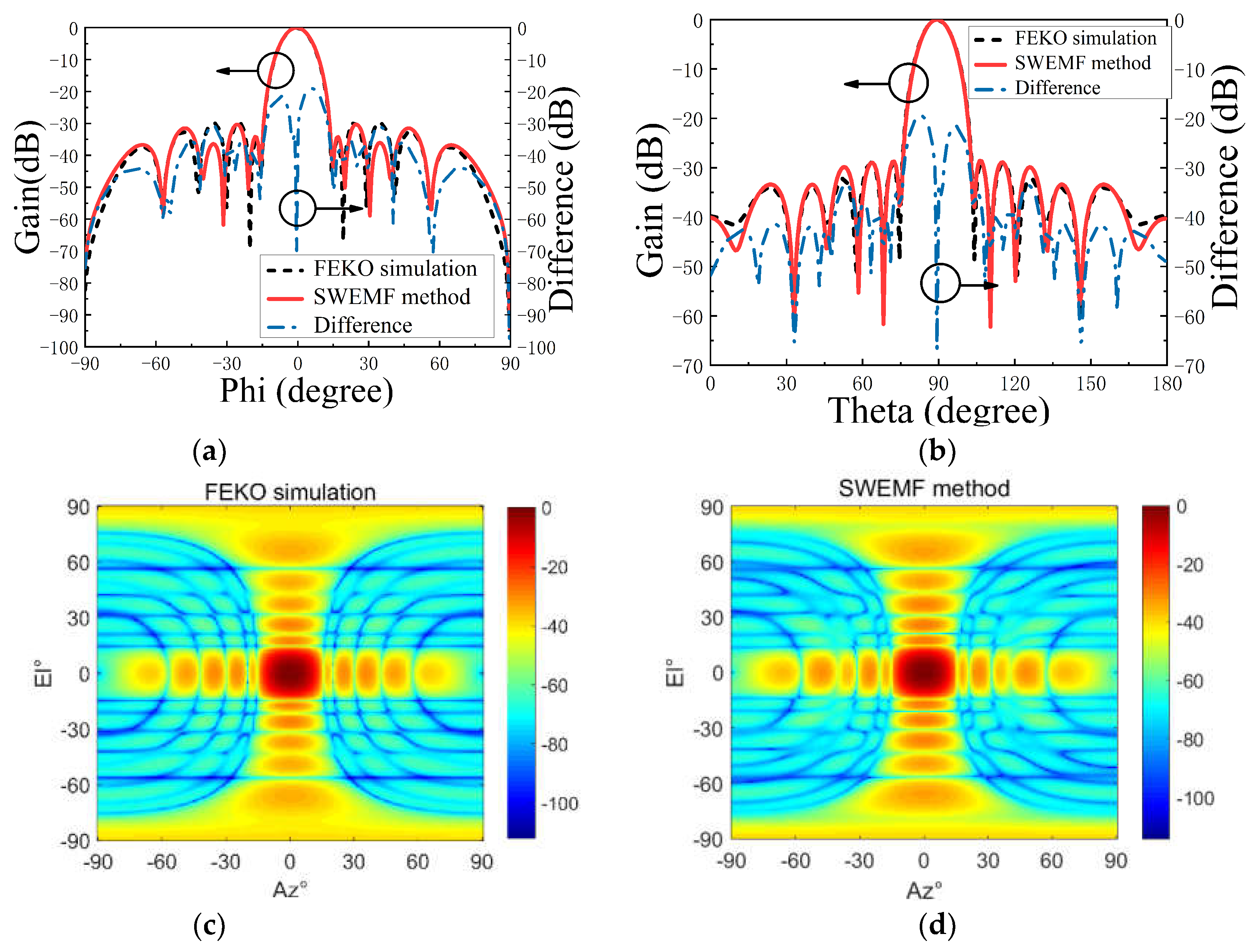
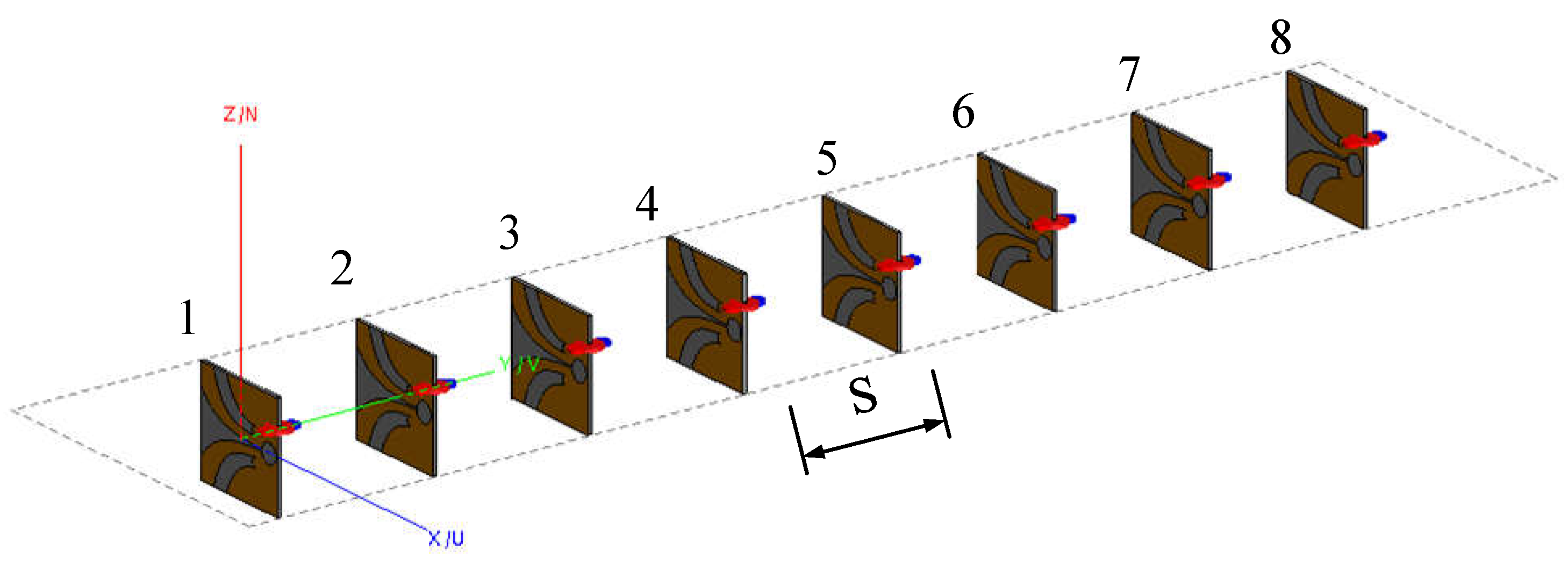
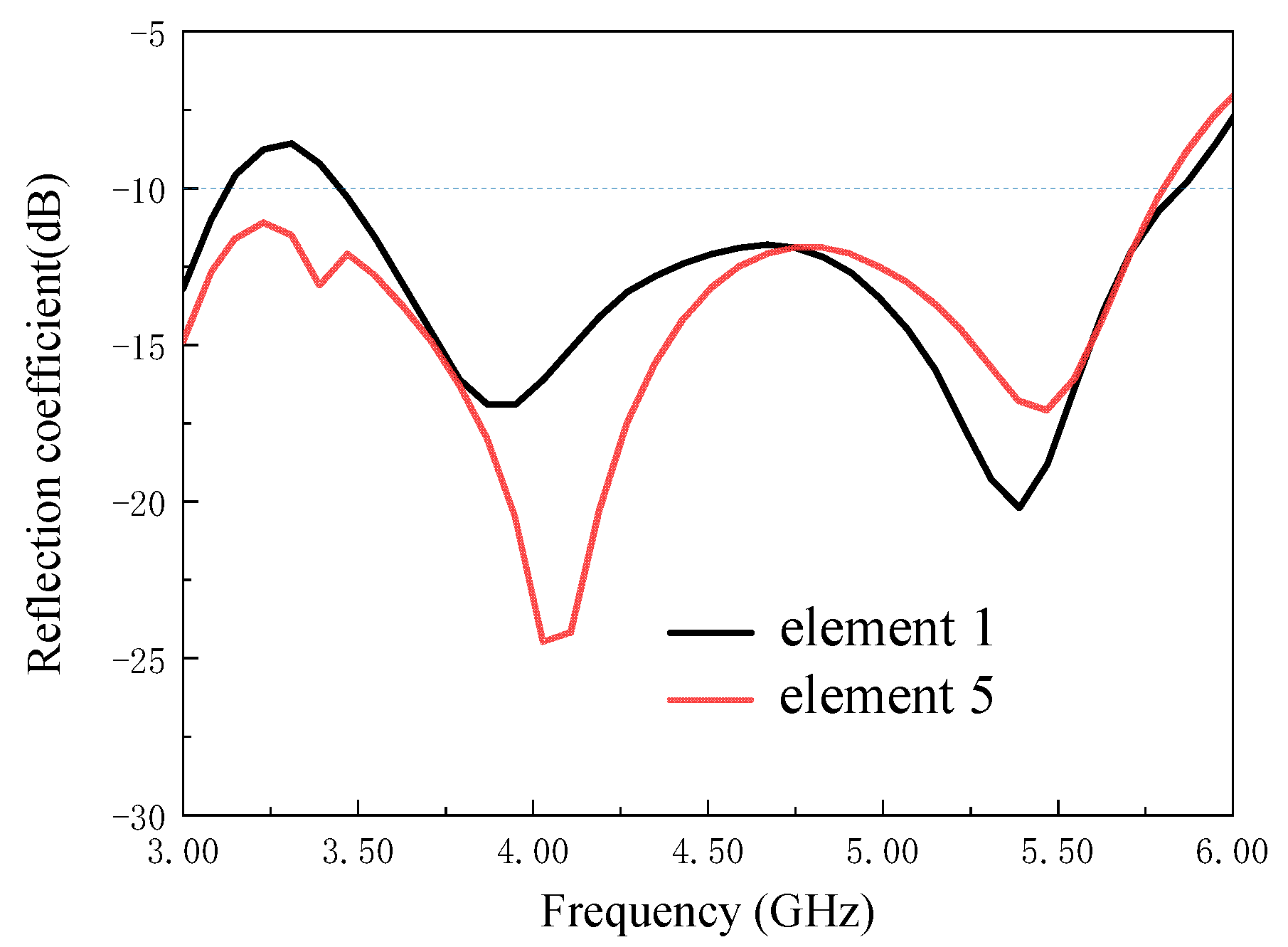
3.3. Vivaldi Linear Array

Figure 8 shows a single Vivaldi antenna model simulated by HFSS:
where W = 30 mm and L = 30 mm. The operating frequency is 5 GHz. The antenna units are vertically and equidistant along the positive direction of the y-axis, with a spacing of S = 45 mm. The schematic diagram of antenna array is shown in Figure 9.
Figure 8. Vivaldi antenna model.
Electronics 11 03479 g008
Figure 9. Vivaldi linear array model. Numbers 1–8 are the serial numbers of antenna units.
Electronics 11 03479 g009
Figure 10 is the S parameters of the Vivaldi linear array, and the reflection coefficients of the fifth element in the middle and the first element at the edge are also given.
In the event that the phase shifter of unit 4 of the phased array antenna fails. Set the feed of unit 4 as amplitude 1 V, phase 45 deg, and other units are excited with amplitude 1 V and phase 0 deg. The calculation results are shown in Table 1.
In order to further analyze the results, Figure 11 shows the comparison between the calculated data feeding pattern and the reference pattern.
Suppose that the attenuator failure occurs in units 1 and 5 of the phased array antenna. Set the feed of units 1 and 5 as amplitude 0.7 V and phase 0 deg. Further, other units are excited with amplitude 1 V and phase 0 deg. The calculation results are shown in Table 2.
In order to further analyze the results, Figure 12 shows the comparison between the calculated data feeding pattern and the reference pattern.
The calculated amplitude error of all units is less than 0.05 V, and the phase error is less than 5°. Taking the calculated amplitude and phase as the excitation input model of the phased array antenna, it can be seen that the calculated pattern is essentially consistent with the reference pattern. The above experiments show that the method is effective and can be applied to broadband antenna arrays.
The specific comparison between the SWEMF method and other methods is given in Table 3.
The SWEMF method has great advantages in the number of measurements. It does not require multiple measurements. Further, it only needs to measure the total field of the array once in order to calculate the feed of the units and has no requirements on the feeding system. The SWEMF method has no reverse operation and iterative optimization, it has only one solution and is therefore more accurate. This method can realize the range of feed amplitude error of 0.05 v and the range of phase error of 5.2°. Thus, the accuracy of the result of this method is high. The feed calculation results of the planar low sidelobe dipole array and Vivaldi linear array are all within this error range. This method takes about 60 s to calculate amplitude and phase at a time. As such, this method is a forward calculation, and the radiation field of the antenna element is obtained after coordinate translation, spherical wave expansion and mode filtering. The feed amplitude and phase can be calculated only with the data in a small angular domain, and the amount of data is small.

4. Conclusions

The SWEMF method is a phased array excitation amplitude and phase calculation method based on spherical wave expansion and mode filtering. The SWEMF method proposed in this paper is theoretically applicable to all frequencies. The examples given in this paper prove the accuracy of the method, and the same method is also applicable to other antennas with different operating frequencies. As the mode filtering method has strong frequency adaptability, it is especially suitable for the feed calculation of broadband phased array antenna and has certain advantages. Only the far-field data of the phased array are needed to obtain the excitation amplitude and phase of each element. The SWEMF method does not require inverse operations and optimization iterations. The mode filtering step can filter out the influence of the multipath effect, as such it can be applied to phased array antennas that are inconvenient to disassemble, such as in the case of airplanes, ships, etc. Further, the far-field measurement can be carried out in a non-absorbent environment. As such, the analytical method is theoretically complete and can be applied to phased array antennas of any arbitrarily complex structure.

Author Contributions

Conceptualization, Y.S., S.Z. and S.G.; methodology, Y.S. and Z.S.; formal analysis, Y.S. and S.G.; writing—original draft preparation, Y.S. and Z.S.; writing—review and editing, Y.S., Z.S., S.Z. and S.G.; project administration, Z.S. All authors have read and agreed to the published version of the manuscript.

Funding

This research received no external funding.

Conflicts of Interest

The authors declare no conflict of interest.

References

  1. Jiang, Z.; Huang, J.; Liu, Z.; Zou, D. A method to diagnose the fault of phase array antenna element. In Proceedings of the 2015 12th IEEE International Conference on Electronic Measurement & Instruments (ICEMI), Qingdao, China, 16–18 July 2015; pp. 239–243. [Google Scholar]
  2. Peters, T.J. A conjugate gradient-based algorithm to minimize the sidelobe level of planar arrays with element failures. IEEE Trans. Antennas Propagat. 1991, 39, 1497–1504. [Google Scholar] [CrossRef]
  3. Xiong, C.; Xiao, G. A Diagnosing Method for Phased Antenna Array Element Excitation Amplitude and Phase Failures Using Random Binary Matrices. IEEE Access 2020, 8, 33060–33071. [Google Scholar] [CrossRef]
  4. Mailloux, R.J. (Ed.) Phased Array Antenna Handbook, 2nd ed.; Artech House: Norwood, MA, USA, 2005. [Google Scholar]
  5. Gattoufi, L.; Picard, D.; Rekiouak, A.; Bolomey, J.C. Matrix method for near-field diagnostic techniques of phased arrays. In Proceedings of the International Symposium on Phased Array Systems and Technology, Boston, MA, USA, 15–18 October 1996; pp. 52–57. [Google Scholar]
  6. Yaccarino, R.G.; Rahmat-Samii, Y. Phaseless bi-polar planar near-field measurements and diagnostics of array antennas. IEEE Trans. Antennas Propagat. 1999, 47, 574–583. [Google Scholar] [CrossRef]
  7. Gregson, S.F.; Newell, A.C.; Hindman, G.E.; Carey, M.J. A Pplication of Mathematical Absorber Reflection suppression to planar near-field antenna measurements. In Proceedings of the 5th European Conference on Antennas and Propagation (EUCAP), Rome, Italy, 11–15 April 2011; pp. 3412–3416. [Google Scholar]
  8. Lord, J.A.; Cook, G.G.; Anderson, A.P. Reconstruction of the Excitation of Array Antennas from the Measured Near-Field Intensity using Phase Retrieval. In Proceedings of the 1992 22nd European Microwave Conference, Helsinki, Finland, 5–9 September 1992; pp. 525–530. [Google Scholar]
  9. Gregson, S.F.; Parini, C.G.; Newell, A.C. A General and Effective Mode Filtering Method for the Suppression of Clutter in Far-Field Antenna Measurements. In Proceedings of the 2018 AMTA Proceedings, Williamsburg, VA, USA, 4–9 November 2018; pp. 1–5. [Google Scholar]
  10. Yoon, H.-J.; Min, B.-W. Improved Rotating-Element Electric-Field Vector Method for Fast Far-Field Phased Array Calibration. IEEE Trans. Antennas Propagat. 2021, 69, 8021–8026. [Google Scholar] [CrossRef]
  11. Shang, J.-P.; Li, X.-R.; Sun, L.-C.; Shang, F.-F. A novel fast measurement method and diagnostic of phased array antennas. In Proceedings of the 10th International Symposium on Antennas, Propagation & EM Theory (ISAPE), Xi’an, China, 22–26 October 2012; pp. 219–222. [Google Scholar]
  12. Wang, Z.; Zhang, F.; Gao, H.; Franek, O.; Pedersen, G.F.; Fan, W. Over-the-Air Array Calibration of mmWave Phased Array in Beam-Steering Mode Based on Measured Complex Signals. IEEE Trans. Antennas Propagat. 2021, 69, 7876–7888. [Google Scholar] [CrossRef]
  13. Xiong, C.; Xiao, G. A Phased Array Antenna Element Failure Diagnostic Method Using Independent Measurements of Different Phases. In Proceedings of the 2019 IEEE International Conference on Computational Electromagnetics (ICCEM), Shanghai, China, 20–22 March 2019; pp. 1–3. [Google Scholar]
  14. Kuznetsov, G.; Temchenko, V.; Voskresenskiy, D.; Miloserdov, M. Phased antenna array reconstructive diagnostics using small number of measurements. In Proceedings of the 2018 Baltic URSI Symposium (URSI), Poznan, Poland, 15–17 May 2018; pp. 174–177. [Google Scholar]
  15. Hasan, M.M.; Faruque, M.R.I.; Islam, M.T. Beam steering of eye shape metamaterial design on dispersive media by FDTD method. Int. J. Numer. Model. 2018, 31, e2319. [Google Scholar] [CrossRef]
  16. Hasan, M.M.; Faruque, M.R.I.; Islam, M.T. Compact Left-Handed Meta-Atom for S-, C- and Ku-Band Application. Appl. Sci. 2017, 7, 1071. [Google Scholar] [CrossRef] [Green Version]
  17. Hasan, M.M.; Rahman, M.; Faruque, M.R.I.; Islam, M.T.; Khandaker, M.U. Electrically Compact SRR-Loaded Metamaterial Inspired Quad Band Antenna for Bluetooth/WiFi/WLAN/WiMAX System. Electronics 2019, 8, 790. [Google Scholar] [CrossRef] [Green Version]
  18. Hasan, M.M.; Faruque, M.R.I.; Islam, M.T. Dual Band Metamaterial Antenna For LTE/Bluetooth/WiMAX System. Sci. Rep. 2018, 8, 1240. [Google Scholar] [CrossRef] [Green Version]
  19. Nguyen, Q.M.; Dang, V.; Kilic, O. An Alternative Plane Wave Decomposition of Electromagnetic Fields Using the Spherical Wave Expansion Technique. IEEE Antennas Wirel. Propag. Lett. 2017, 16, 153–156. [Google Scholar]
  20. Gemmer, T.M.; Heberling, D. Accurate and Efficient Computation of Antenna Measurements Via Spherical Wave Expansion. IEEE Trans. Antennas Propagat. 2020, 68, 8266–8269. [Google Scholar] [CrossRef]
  21. Gregson, S.F.; Dupuy, J.; Parini, C.G.; Newell, A.C.; Hindman, G.E. Application of Mathematical Absorber Reflection Suppression to far-field antenna measurements. In Proceedings of the 2011 Loughborough Antennas & Propagation Conference, Loughborough, UK, 14–15 November 2011; pp. 1–4. [Google Scholar]
  22. Gregson, S.F.; Tian, Z. Verification of Generalized Far-Field Mode Filtering Based Reflection Suppression Through Computational Electromagnetic Simulation. In Proceedings of the 2020 IEEE International Symposium on Antennas and Propagation and North American Radio Science Meeting, Montreal, QC, Canada, 5–10 July 2020; pp. 2059–2060. [Google Scholar]
  23. Hess, D.W. The IsoFilterTM Technique: A Method of Isolating the Pattern of an Individual Radiator from Data Measured in a Contaminated Environment. IEEE Antennas Propag Mag. 2010, 52, 174–181. [Google Scholar] [CrossRef]
  24. Gregson, S.F.; Tian, Z. Comparison of Spherical and Cylindrical Mode Filtering Techniques for Reflection Suppression With mm-wave Antenna Measurements. In Proceedings of the 2018 IEEE Conference on Antenna Measurements & Applications (CAMA), Västerås, Sweden, 3–6 September 2018; pp. 1–4. [Google Scholar]
  25. Thal, H.L.; Manges, J.B. Theory and practice for a spherical-scan near-field antenna range. IEEE Trans. Antennas Propag. 1988, 36, 815–821. [Google Scholar] [CrossRef]
Figure 1. Schematic diagram of the mode filtering geometry of a planar array antenna.
Electronics 11 03479 g001
Figure 2. Flowchart of the SWEMF method.
Electronics 11 03479 g002
Figure 3. Extraction results of the radiation field of 1–4 elements on the phi = 0° surface. (a) Element 1, (b) element 2, (c) element 3 and (d) element 4.
Electronics 11 03479 g003
Figure 4. Comparison of the pattern of the FEKO-simulated dipole linear array and the pattern obtained by the SWEMF method.
Electronics 11 03479 g004
Figure 5. The S parameter of the 10 × 10 dipole planar array.
Electronics 11 03479 g005
Figure 6. Calculation results of element excitation amplitude and phase. (a) Calculated feed amplitude as compared to given amplitude and (b) calculated feed phase as compared to the given phase.
Electronics 11 03479 g006
Figure 7. Comparison of the pattern of the FEKO simulated plane array and the pattern obtained by the SWEMF method. (a) Theta = 90° surface, (b) Phi = 0° surface, (c) pattern simulated by FEKO and (d) pattern calculated by the SWEMF method.
Electronics 11 03479 g007
Figure 10. S parameter of Vivaldi linear array.
Electronics 11 03479 g010
Figure 11. Comparison between the calculated pattern and the reference pattern.
Electronics 11 03479 g011
Figure 12. Comparison between the calculated pattern and the reference pattern.
Electronics 11 03479 g012
Table 1. The initial feed and the calculated feed amplitude and phase.
Order
Number
Reference
Amplitude/V
Calculated
Amplitude/V
Error of
Amplitude/V
Reference
Phase/deg
Calculated
Phase/deg
Error of
Phase/deg
111.01690.01690−0.94220.9422
211.01930.019304.34004.3400
310.97600.02400−0.79410.7941
410.95550.04454541.73263.2674
510.97640.02360−1.23321.2332
611.02670.026704.45614.4561
711.01030.01030−0.88670.8867
810.98220.01780−2.50322.5032
Table 2. The initial feed and the calculated feed amplitude and phase.
Order
Number
Reference
Amplitude/V
Calculated
Amplitude/V
Error of
Amplitude/V
Reference
Phase/deg
Calculated
Phase/deg
Error of
Phase/deg
10.70.72010.02010−2.982.98
211.03200.03200−3.31723.3172
310.95980.040201.84951.8495
411.02300.023002.07162.0716
50.70.70080.00080−1.44771.4477
611.03210.03210−2.90932.9093
710.97550.024501.05611.0561
811.01010.010101.41651.4165
Table 3. Comparison of different methods.
Number of
Measurements
EfficiencyTesting EnvironmentTest Site
SWEMF method1Test all units in one test.Non absorbing environment or absorbing environmentFar field or near field
REV method2M*NTest one or more units in one testAbsorbing environmentFar field or near field or antenna aperture
Phase-shift measurement method2M*NTest all units in one test.Absorbing environmentFar field or near field
Compressed sensing-based (CS) methodNTest one unit in one test.Absorbing environmentFar field
Where M is the digit of the phase shifter and N is the number of array elements.
Publisher’s Note: MDPI stays neutral with regard to jurisdictional claims in published maps and institutional affiliations.

