High Density Sensor Networks Intrusion Detection System for Anomaly Intruders Using the Slime Mould Algorithm

Abstract

The Intrusion Detection System (IDS) is an important feature that should be integrated in high density sensor networks, particularly in wireless sensor networks (WSNs). Dynamic routing information communication and an unprotected public media make them easy targets for a wide variety of security threats. IDSs are helpful tools that can detect and prevent system vulnerabilities in a network. Unfortunately, there is no possibility to construct advanced protective measures within the basic infrastructure of the WSN. There seem to be a variety of machine learning (ML) approaches that are used to combat the infiltration issues plaguing WSNs. The Slime Mould Algorithm (SMA) is a recently suggested ML approach for optimization problems. Therefore, in this paper, SMA will be integrated into an IDS for WSN for anomaly detection. The SMA’s role is to reduce the number of features in the dataset from 41 to five features. The classification was accomplished by two methods, Support Vector Machine with polynomial core and decision tree. The SMA showed comparable results based on the NSL-KDD dataset, where 99.39%, 0.61%, 99.36%, 99.42%, 99.33%, 0.58%, and 99.34%, corresponding to accuracy, error rate, sensitivity, specificity, precision, false positive rate, and F-measure, respectively, are obtained, which are significantly improved values when compared to other works.

1. Introduction

Sensing data (light, vibration, temperature, etc.) can be collected via a sensor network, which consists of a dispersed collection of sensor nodes in communication with one another and a central base station node. A sensor network is known as a wireless sensor network if its communications are wireless (WSN). There have been several applications of WSNs ever since their inception [1]. WSNs have found widespread use in fields as diverse as animal monitoring [2], ecological studies [3], volcanic observation [4], water observation [5], and so on. However, WSNs have their own unique challenges due to their design. For instance, a sensor node’s lifetime is constrained by the battery attached to it, and the network’s lifetime is contingent on the lifetime of sensor nodes; therefore, it is often recommended to take energy efficiency into account in a WSN design to further reduce maintenance and redeployment costs [6]. However, there are several complications that need to be taken into account while designing a network to accommodate the requirements provided by sensor information gathering systems. For starters, the installed sensors might have to cover the full region of interest for the sensor data gathering application. It’s possible that strategically positioned sensors will be required to gather data from certain locations. Data may be collected from a wide variety of sources thanks to sensors with a wide range of sampling rates. These issues, if left unchecked, might lead to unequal use of energy across a WSN, which would significantly shorten the lifespan of the system. Sending data to the base station without introducing any errors makes data accumulation procedures challenging to accomplish, calling for creative approaches to improve network performance [7].

WSNs have many drawbacks, the most serious of which is their lack of security. As discussed before, WSNs are built up from a vast network of physical sensors, or nodes, that are dispersed around the study area. The most crucial information is gathered by these nodes and sent to the base station, also known as the sink node [8]. In other words, data will be sent throughout the WSN in accordance with predetermined protocols [9]. Wireless communication is best since sensors are in regions where wired connectivity is difficult [10]. To securely transfer data, WSNs must be protected from intruders. To achieve this task, multiple WSN resources must be accessible, but they are restricted due to energy, memory, processing capability, and other restrictions [11]. Because of these restrictions, cryptography is difficult to implement [9]. Due to their open, scattered nature and limited sensor node properties, WSNs are vulnerable to attacks. WSNs frequently need packet broadcasting, and sensor nodes can be placed at random, allowing an attacker to swiftly enter [12].

If a hacker controls a sensor, they may snoop, broadcast fake information, change or corrupt information, and eat up network resources. DoS attacks are a widespread and severe threat to WSNs. Attackers utilize several strategies to stop WSN capabilities [13]. Because avoiding or mitigating security threats is not always possible, an IDS is essential to identify known and new assaults and warn sensor nodes [11]. IDSs can be categorized as patterns or statistical abnormalities. Signature-based IDS may uncover known attack patterns in their fingerprints [14]. Pattern recognition IDS cannot detect attacks without signatures in the IDS library. In anomaly-based IDS, profiles of usual actions are stored in the repository. Within those solutions, all network actions are carefully monitored and assessed. Any divergence from regular behavior is considered an attack. Anomaly-based systems can discover unknown dangers. False positives are typical in these systems because strange patterns are highlighted as potential assaults even though they are not [15].

Moreover, IDS effectiveness is enhanced by employing a wide variety of machine learning (ML) and nature-inspired metaheuristic techniques [16]. Nature-inspired techniques, such as particle swarm optimization (PSO) and artificial bee colonies (ABC) [17,18], have been employed to improve IDS performance in recent years. The Slime Mould Algorithm (SMA) [19] will be used to construct the IDS in this study. The recommended structure of the slime mould oscillation mode (SMA) is inspired by the inherent oscillation form of slime mould. A novel mathematical model is used to mimic the methodology of creating constructive and destructive feedback of the dispersion pattern of slime mould, relying on a bio-oscillator to build the ideal route for linking foodstuffs, having an outstanding exploration capability and exploitative tendency.

Feature selection (FS) is a method for improving the categorization of patterns by eliminating superfluous features and selecting the most informative ones. Due to the ever-increasing complexity of data, feature selection as a preprocessing phase is gaining prominence in the evolution of IDS [20,21]. Because of this, the dimensionality of the dataset has to be decreased in order to get rid of any unneeded information. To put it another way, the datasets that are provided by the IDS contain a significant number of dimensions that are either pointless or unnecessary. This causes a slow rate of detection and results in poor functionality. As a direct consequence of this, FS has been incorporated into IDS in order to reduce dimensionality. For example, a methodology for IDS based on GAs has been described by [22]. In this method, correlation-based FS is employed to determine the optimal solution throughout the operation of selecting features. In the paper [23], the authors utilize an improved version of the bat method to do FS. Then, they apply the k-means clustering approach to break the entire swarm up into subgroups. This allows each subgroup to learn more efficiently both within and across different populations. Utilizing binary differential mutation is another method that may be utilized to broaden the scope of available experience. In [24], the authors introduced a new method of Geometric Area Analysis that uses Trapezoidal Area Estimation with each sample based on the Beta Mixture Model for features and relationships across records. By correlating each record to predetermined intervals, this flexible and compact anomaly-based approach may identify attacks; also, normal activities have been stored as a regular pattern during the training period. A concept for multi-objective FS is proposed in [25]. The model evaluates the effectiveness of the FS method from many standpoints, including the optimality of the selected feature count, FAR, true positive rate, precision, and accuracy. At the same time, an approach for optimal optimization for achieving several different goals at once is being created as a means of solving this model. For greater convergence and variety, after constructing the evolution strategy pool and the dominance strategy pool, the algorithm will proceed to pick a strategy from one of the available options by employing a random chance strategy selection process.

The authors in [26] offer a feature selection strategy for selecting the best features to include in the final product. Next, these subsets are sent to the suggested hybrid ensemble learning, which also uses minimal computational and time resources to increase the IDS’s stability and accuracy. This research is important since it seeks to: decrease the dimensionality of the CICIDS2017 dataset by combining Correlation Feature Selection and Forest Panelized Attributes (CFS–FPA); determine the optimal machine learning strategy for aggregating the four modified classifiers (SVM, Random Forests, Naïve Bayes, and K-Nearest Neighbor (KNN)); and validate the effectiveness of the hybrid ensemble scheme. We must examine the CFS–FPA and other feature selection methods with regard to accuracy, detections, and false alarms. Ultimately, the results will be employed to extend the effectiveness of the suggested feature selection method. We can evaluate how each of the classification techniques performed prior to and after being modified to use the AdaBoosting technique. Further, they will evaluate the recommended methodology against alternative available options.

Proximal policy optimization (PPO) is used in [27] to present an intrusion detection hyperparameter control system (IDHCS) that trains a deep neural network (DNN) feature extractor and a k-means clustering component under the control of the DNN. Intruders can be detected using k-means clustering, and the IDHCS ensures that the strongest useful attributes are extracted from the network architecture by controlling the DNN feature extractor. Automatically, performance improvements tailored to the network context in which the IDHCS is deployed are achieved by iterative learning utilizing a PPO-based reinforcement learning approach. To test the efficacy of the methodology, researchers ran simulations with the CICIDS2017 as well as UNSW-NB15 databases. An F1-score of 0.96552 has been attained in CICIDS2017, whereas an F1-score of 0.94268 has been attained in UNSW-NB15. As a test, they combined the two data sets to create a larger, more realistic scenario. The variety and complexity of the attacks seen in the study increased after integrating the records. When contrasted to CICIDS2017 and UNSW-NB15, the combined dataset received an F1 score of 0.93567, suggesting performance between 97% and 99%. The outcomes demonstrate that the recommended IDHCS enhanced the IDS’s effectiveness through the automated learning of new forms of attacks via the management of intrusion detection attributes independent of the changes in the network environment.

In this research [28], researchers present an ML-based IDS for use in a practical industry to identify DDoS attacks. They acquire innocuous data from Infineon’s semiconductor manufacturing plants, such as network traffic statistics. They mine the DDoSDB database maintained by the University of Twente for fingerprints and examples of real-world DDoS assaults. To train eight supervised learning algorithms—LR, NB, Bayesian Network (BN), KNN, DT, Random Forest (RF), and Classifier—we can employ feature selection techniques such as Principal Component Analysis (PCA) to lower the dimensionality of the input. The authors then investigated one semi-supervised/statistical classifier, the univariate Gaussian algorithm, and two unsupervised learning algorithms, simple K-Means and expectation maximization (EM). This is the first study that researchers are aware of that uses data collected from an actual factory to build ML models for identifying DDoS attacks in industry. Some works have applied ML to the problem of detecting distributed denial-of-service (DDoS) attacks in operational technology (OT) networks, but these approaches have relied on data that was either synthesized for the purpose or collected from an IT network.

Jaw and Wang introduced hybrid feature selection (HFS) using an ensemble classifier in their paper [29]. This method picks relevant features in an effective manner and offers a classification that is compatible with the attack. Initially. For instance, it outperformed all of the selected individual classification methods, cutting-edge FS, and some current IDS methodologies, achieving an amazing outcome accuracy of 99.99%, 99.73%, and 99.997%, and a detection rate of 99.75%, 96.64%, and 99.93%, respectively, for CIC-IDS2017, NSL-KDD, and UNSW-NB15, respectively. The findings, on the other hand, are dependent on 11, 8, and 13 pertinent attributes that were chosen from the dataset.

Researchers give a review of IDSs in [30] that looks at them from the point of view of ML. They discuss the three primary obstacles that an IDS faces in general, as well as the difficulties that an IDS faces for the internet of things (IoT) specifically; these difficulties are idea drift, high dimensionality, and high computational. The orientation of continued research as well as studies aimed at finding solutions to each difficulty are discussed. In addition, the authors have devoted an entirely separate section of this study to the presentation of datasets that are associated with an IDS. In particular, the KDD99 dataset, the NSL dataset, and the Kyoto dataset are shown herein. This article comes to the conclusion that there are three aspects of concept drift, elevated number of features, and computational awareness that are symmetric in their impact and need to be resolved in the neural network based concept for an IDS in the internet of things (IoT).

Using the Weka tool and 10-fold cross-validation with and without feature selection/reduction techniques, the authors of [31] assessed six supervised classifiers on the entire NSL-KDD training dataset. The study’s authors set out to find new ways to improve upon and protect classifiers that boast the best detection accuracy and the quickest model-building times. It is clear from the results that using a feature selection/reduction technique, such as the wrapper method in conjunction with the discretize filter, the filter method in conjunction with the discretize filter, or just the discretize filter, can drastically cut down on the time spent on model construction without sacrificing detection precision.

Auto-Encoder (AE) and PCA are the two methods that Abdulhammed et al. [32] utilize to reduce the dimensionality of the features. The low-dimensional features that are produced as a result of applying either method are then put to use in the process of designing an intrusion detection system by being incorporated into different classifiers, such as RF, Bayesian Networks, Linear Discriminant Analysis (LDA), and Quadratic Discriminant Analysis. The outcomes of the experiments with binary and multi-class categorization using low-dimensional features demonstrate higher performance in terms of detection rate, F-Measure, false alarm rate, and accuracy. This investigation endeavor was successful in lowering the number of feature dimensions in the CICIDS2017 dataset from 81 to 10, while still achieving an accuracy rate of 99.6% in both multi-class and binary classification. A new IDS based on random neural networks and ABC is proposed in article [33] (RNN-ABC). Using the standard NSL-KDD data set, researchers train and evaluate the model. The recommended RNN-ABC is compared to the conventional RNN trained with the gradient descent approach on a variety of metrics, including accuracy. Still, maintaining a 95.02% accuracy rate generally

An experimental IDS built on ML is presented in [34]. The proposed approach is computationally efficient without sacrificing detection precision. In this study, researchers examine how different oversampling techniques affect the required training sample size for a given model, and then find the smallest feasible training record group. Approaches for optimizing the IDS’s performance depending on its hyperparameters are currently under investigation. Using the NSL-KDD dataset, the created system’s effectiveness is verified. The experimental results show that the suggested approach cuts down on the size of the feature set by 50% (20-featured), while also decreasing the amount of mandate elements by 74%.

Using a convolutional neural network to obtain sequence attributes of data traffic, whereupon reassigning the weights of each channel using attention methodology, and eventually utilizing bidirectional long short-term memory (Bi-LSTM) to learn the architecture of sequence attributes, this study recommends a conceptual framework for traffic outlier recognition called a deep learning algorithm for IDS. A great deal of data inconsistency is present in publicly available IDS databases. Hence, the study in [35] utilizes a redesigned stacked autoencoder for data feature reduction with the goal of improving knowledge integration, and it leverages adaptive synthetic sampling for sample enlargement of minority category observations to ultimately generate a fairly balanced dataset. Since the deep learning algorithm for the IDS methodology is a full-stack structure, it does not require any human intervention in the form of extraction of features. Study findings reveal that this technique outperforms existing techniques of comparison on the public standard dataset for IDS, NSL-KDD, with an accuracy of 90.73% and an F1-measure of 89.65%.

Using an χ2 statistical approach and Bi-LSTM, the authors of [36] suggest a new feature-driven IDS called χ2-Bi-LSTM. The χ2-Bi-LSTM process begins by ranking all the characteristics with an χ2 approach, and then employing an upwards-leading search method, it looks for the optimal subset. The final step involves feeding the ideal set to a Bi-LSTM framework for categorization. The empirical findings show that the suggested χ2-Bi-LSTM technique outperforms the conventional LSTM technique and perhaps various available attribute IDS approaches on the NSL-KDD dataset, with an accuracy rate of 95.62%, an F-score of 95.65%, and a minimal FPR of 2.11%. Li et al. recommended a smart IDS for software-defined 5G networks in [37]. Taking advantage of software-defined technologies, it unifies the invocation and administration of the various security-related function modules into a common framework. In addition, it makes use of ML to automatically acquire rules through massive amounts of information and to identify unexpected assaults by utilizing flow categorization. During flow categorization, it employs a hybrid of k-means and adaptive boosting (AdaBoost) and uses RF for FS. There will be a significant increase in security for upcoming 5G networks with the adoption of the suggested solution as per the authors.

However, the plasmodium creates an efficient network of protoplasmic tubes linking the masses of protoplasm to the feed ingredients. During the phase of translocation, the front end spreads out like a fan, and veins that are related to one another and to the rest of the body follow behind, allowing cytoplasm to flow within. Molds secrete enzymes to capture the food locations as they move through their venous network hunting for food. When food is scarce, slime mold may actually flourish, which provides insight into how slime mold searches for, travels through, and connects to food in its ever-evolving environment. Slime can evaluate the positive and negative signals it receives when a secretion approaches its target, allowing it to find the best path to grip food. This indicates that, depending on the availability of food, slime mold can lay down a solid concrete walkway. The area with the greatest concentration of food is the one it chooses most often. In the course of foraging, molds evaluate the availability of food and the safety of their immediate surroundings, and then determine how quickly to abandon their current site in favor of a new one. When deciding when to start a fresh search and leave its existing position, slime mold uses empirical principles based on the limited information it has at the time. Mold may split its biomass to make use of several resources based on the knowledge of a rich, high-quality food supply, even if it is abundant. It is possible that it might dynamically modify its search strategies in response to changes in the availability of food.

To the best knowledge of the authors, the SMA was not previously employed as an FS in an IDS; that is, in this paper, the SMA methodology is proposed for FS. Thus, the 41-features of the NSL-KDD dataset may include redundant features or useless features; hence, feature reduction using the SMA will be used to reduce this number of features. To achieve this goal, a classifier should be integrated into the SMA technique. Therefore, the KNN algorithm has been chosen as a classifier to be used as an evaluation approach in the SMA because it is the algorithm with the least amount of complexity and the most straightforward integration. This prevents the design process from becoming more convoluted. Then, after the feature selection process is accomplished, an ensemble of classification methodologies will be implemented, which will be SVM polynomial core and the DT classification method.

The rest of this paper is organized as follows: the next section, Section 2, provides the mathematical model of the SMA algorithm and its operation. In Section 2, also the dataset used in this work will be described, which is the NSL-KDD dataset [38]. The binary classifications, SVM and decision tree (DT), will be discussed, which will be utilized for binary classification of the intruders. The evaluation metrics will be drawn from the confusion matrix, such as accuracy, error rate, detection rate, FPR, TNR, precision, and F-measure, all in Section 3 introduces the discussion of the obtained results. Last but not least, Section 4 shows the concluding remarks highlighted in this work.

2. Materials and Methods

The employed dataset in this article will be described in this section. Furthermore, the methodology that is utilized for the FS process will be discussed as well as the classification tools.

2.1. NSL-KDD Dataset Description

Researchers in both academia and business employ the NSL-KDD dataset [39], which is deployed as a modernized version of the dataset known as the KDD CUP 99 [40], since it is more trustworthy. For each entry, you will find support for 41 different attributes, any of which may be assigned to the record’s attack type or its normal type. Attribute values can be either nominal, binary, or numeric. However, unlike the KDD CUP 99, the NSL-KDD dataset’s training set does not contain any duplicate entries; therefore, classifiers will not be biased toward more frequent records. Therefore, in NSL-KDD, the techniques with better detection rates of the frequent records in test sets do not affect the performance of learners. That is, the 41 features available in this dataset have three nominal-type features, Protocol_type, Service, and Flag, while the others are all of type-double, as shown in

Table 1. NSL-KDD dataset Types of features.

Feature	Type
Duration, src_bytes, dst_bytes, land, wrong_fragment, urgent, hot, num_failed_logins, logged_in, num_compromised, root_shell, su_attempted, num_root, num_file_creations, num_shells, num_access_files, num_outbound_cmds, is_host_login, is_guest_login, count, srv_count, serror_rate, srv_serror_rate, rerror_rate, srv_rerror_rate, same_srv_rate, diff_srv_rate, srv_diff_host_rate, dst_host_count, dst_host_srv_count, dst_host_same_srv_rate, dst_host_diff_srv_rate, dst_host_same_src_port_rate, dst_host_srv_diff_host_rate, dst_host_serror_rate, dst_host_srv_serror_rate, dst_host_rerror_rate and dst_host_srv_rerror_rate.	double
“Protocol_type”, “Service”, and “Flag”.	Nominal

.

Label and level are two more features that may be found in the NSL-KDD dataset. These are the other two attributes. While the level reveals the extent of the attack, the label property categorizes the record as either an attack or a typical occurrence. Further in, the attack attribute contains an excessive number of kinds, including normal, which indicates that the communication is not being attacked, and a wide variety of additional values, such as nmap, Neptune, multihop, loadmodule, etc. Figure 1 displays all of the potential values for the label attribute that can be found in the training file for the NSL-KDD collection.

Denial of service (DoS), remote-to-local (R2L), user-to-root (U2R), and probing attacks are the four main categories of cyberattacks. In this study, categorization will be performed using binary labels, meaning that all values associated with the label attribute will be transformed into either attack or safe. In this work, the SMA will be integrated into the suggested IDS; that is, FS will be conducted using the SMA to reduce the number of utilized features, and then a classifier will be built to classify the samples as either attack or normal/safe.

2.2. Methods

2.2.1. The Slime Mould Algorithm Mathematical Model

Slime mold activity is modeled mathematically, and a rule is established for determining the organism’s current location while it searches for food. The relevant criteria are r- and p-dependent. Mold’s method of shrinkage looks like this [19]:

$$X\left(t+1\right)=\{\begin{array}{cc}{X}_b\left(t\right)+vb·\left(W·X_A\left(t\right)-X_B\left(t\right)\right)& r<p\\ vc·X\left(t\right)& r\ge p\end{array}$$

(1)

in which, $vb$ is determined as follows:

$$vb=\left[-a,a\right]$$

(2)

where

$$a={\tan \mathrm{h}}^{-1}\left(-\left(\frac{t}{\mathrm{m}t}\right)+1\right)$$

(3)

Hence, in (1), $vc$ is a parameter that decreases linearly from its maximum value, which is one, to zero. $t$ stands for the present iteration, further, $X_b$ corresponds to the highest odor concentration of the individual location currently found, moreover, $X$ refers to the slime mould location. Moreover, there are two individuals that are selected in a random manner from the swarm given as $X_A$ and $X_B$, mt is the maximum iteration count, and the slime mould weight is denoted as $W$, while p is calculated as,

$$p=\tanh \left|S\left(i\right)-DF\right|$$

(4)

In the last expression, i belongs to [1, 2, 3, … n], the fitness of $X$ is denoted as $S\left(i\right)$, while the best fitness is $DF$, which is found within all of the iterations. An excellent visual representation of the SMA mechanism is shown in [19].

However, the weighting function, W, can be calculated as follows:

$$\overrightarrow{W\left(SmellIndex\left(i\right)\right)}=\{\begin{array}{c}1+rnd·\log \left(\frac{bF-S\left(i\right)}{bF-wF}+1\right), condi\\ 1-rnd·\log \left(\frac{bF-S\left(i\right)}{bF-wF}+1\right), others\end{array}$$

(5)

where

$$SmellIndex=sort\left(S\right)$$

(6)

If condi is valid, then $S\left(i\right)$ ranks in the upper fifty percent of the whole population, $rnd$ stands for the value chosen at random from the range [0,1], $bF$ and $wF$ indicate the highest and lowest fitness levels achieved in the current iteration, respectively. On the other hand, $S$ will be sorted in an ascending manner if the problem is to find the minimum value and descending if the problem is to find the maximum value (maximization) as in (6), which is called $SmellIndex$.

The seeking individual X’s position may be revised according to the most optimal position X_b currently discovered, and the fine-tuning of factors vb, vc, and W can modify the participant’s location. The constituents of the equation are able to construct query trajectories at whatever orientation due to the randomness behavior of the rnd function, that is, explore optimum solutions in any direction in order for the algorithm to be able to find the optimal answer. Consequently, (1) allows participants seeking to investigate as many possible opportunities as they can on the way to finding the best answer, imitating the rounded sector architecture of slime mold while imminent food. Up to this level, the approaching food step is done.

During the searching process, this component computationally models the shrinkage mode of the venous tissue arrangement of slime mould. The greater the concentration of food that is brought into contact with the vein, the more powerful the wave that is produced by the bio-oscillator, the more quickly the cytoplasm moves, and the more substantial the vein. This step is called wrapping food. Equation (5) arithmetically reproduced the positive and/or negative feedback regarding the vein thickness of the slime mould and the food content that was investigated. The quantity rnd in (5) replicates the variability of the venous contracting mode. The logarithmic function is integrated in the equation to reduce the rate of change of numeric data such that the quantity of shrinkage rate does not really vary by large amounts. Condi mimics slime mould to modify their hunting methods based on the superiority of food. When the food ranks are elevated, the weight of the region increases; when the food content is poor, the weight of the area declines, causing it to turn to explore other places.

The arithmetic method for adjusting the situation of slime mould is as follows, on the basis of the previously indicated idea:

$$X^{*}=\{\begin{array}{l}rnd·\left(UB-LB\right)+LB,rnd<z\\ X_b\left(t\right)+vb·\left(W·X_A\left(t\right)-X_B\left(t\right)\right),rnd<p\\ vc·X\left(t\right), rnd\ge p\end{array}$$

(7)

where UB is the upper bound of the search range, LB is the lower, and rnd is a random number between 0 and 1. However, z is the exploration control parameter; thus, it can be set according to the problem environments. The slime mould depends greatly on the diffusion flood produced by the bio oscillation in order to cause changes in the cytoplasmic flow in veins, putting them in a more advantageous location in terms of food concentration. Variations in slime mould venous width were simulated using W, vb, and vc to represent the corresponding dimensional changes. Using pseudo-code, Algorithm 1 demonstrates the SMA.

Algorithm 1 Pseudo-code of SMA [19]

Initialize the parameters popsize, $Max\_iteraition$; Establish the starting places for the slime mould $X_i\left(i=1,2,\dots ,n\right)$; While ($t\le Max\mathrm{No}.\mathrm{Iterations})$   Compute the vitality of every type of slime mould (fitness computation); $Update bestFitness, X_b$   Compute W by Equation (5);   For $each search part$   $Update p,vb, vc$;   $Update locations by \mathrm{Equation} \left(7\right)$;   End $For$   $t=t+1$; End While Return $bestFitness, X_b$;

2.2.2. Classification Tools and Evaluation Parameters

In this section, the evaluation parameters to assess the suggested SMA will be discussed. However, the evaluation parameters are the results of the SVM (with polynomial core) and DT. In other words, after the employment of the SMA to reduce the dimensionality of the NSL-KDD dataset, SVM and DT will be used for the classification process. The results are either attack or normal. These two findings will be given as a confusion matrix. Though, from this confusion matrix, different measurement parameters can be shown. Mathematically, they can be given in the next subsequent discussion. For instance, the accuracy of the classifier can be expressed as:

$$Accuracy=\frac{correct predicted samples}{total number of samples}$$

(8)

In other words, the accuracy is the ratio of total samples correctly predicted with respect to the total number of records in the dataset. The correctly predicted records may be attacks; hence, they are called True Positive (TP), and they may be normal records, known as True Negative (TN). In that way, the last expression can be re-arranged,

$$Accuracy=\frac{\mathrm{TP}+\mathrm{TN}}{\mathrm{TP}+\mathrm{TN}+\mathrm{FP}+\mathrm{FN}}$$

(9)

where FP and FN are false positive prediction and false negative classification. To know the rate of false positive prediction (FPR), the following formulation can be used:

$$FPR=\frac{\mathrm{FP}}{\mathrm{TN}+\mathrm{FP}}$$

(10)

While the true positive rate (TPR), aka sensitivity, can be expressed as:

$$TPR=\frac{\mathrm{TP}}{\mathrm{TP}+\mathrm{FN}}$$

(11)

The true negative rate (TNR), aka specificity, can be determined from:

$$TNR=\frac{\mathrm{TN}}{\mathrm{TN}+\mathrm{FP}}$$

(12)

Accordingly, the overall error rate can be expressed as:

$$Error Rate=\frac{\mathrm{FN}+\mathrm{FP}}{\mathrm{TP}+\mathrm{FN}+\mathrm{TN}+\mathrm{FP}}$$

(13)

In contrast, the precision can be determined from:

$$Precision=\frac{\mathrm{TP}}{\mathrm{TP}+\mathrm{FP}}$$

(14)

Last, but not least, the F-measure is a statistical indicator of success that describes how well the recommended strategy classifies data from the NSL-KDD dataset. Specifically, this criterion for assessment might be stated as:

$$F_m=\frac{2\times \mathrm{TP}}{2\times \mathrm{TP}+\mathrm{FP}+\mathrm{FN}}$$

(15)

The parameters listed in (9–15) will be calculated and discussed in the next section to show the power of the suggested methodology.

3. Results and Discussion

One of the noticeable weaknesses of the SMA algorithm is the premature problem [19]. The SMA could come with some downsides, for instance, becoming confined to limited local areas and having an inappropriate equilibrium among the exploitation and discovery rounds of the process [41]. Nevertheless, to overcome this problem, the simulation parameters have to be carefully set. Furthermore, the data should be preprocessed, such as normalization and cleaning. Otherwise, the algorithm will suffer from a prematuring problem. Extensive simulations have been conducted in order to find the best settings to be utilized in our final experiments.

One of the most important parameters that has been set during this phase is the number of neighbors of the KNN classifier, K. Using the SMA is an advantageous way since it is a nature-inspired approach and it can be used for the FS portion of the IDS. However, the aim of using the SMA is to reduce the number of attributes, while classification is the job of other classifiers, such as DT and SVM. Even when a novel attacker appears, the SMA can recognize anomalies based on features. In other words, the selected features will be updated as long as there are new anomalies.

However, the KNN algorithm is a straightforward example of the supervised learning subfield of ML. The KNN method makes an assumption about the degree of correspondence between the new instance and the existing examples and places it in the class to which it is very closely related. The KNN algorithm remembers all the information it has and then uses that information to determine how to categorize a new piece of data. This means that the KNN method can be used to quickly and accurately categorize newly-emerging data into a set of predefined categories. While the KNN technique has certain applications in regression, it is most commonly utilized for classification. When it comes to the underlying data, KNN is a non-parametric methodology. In the training phase, the KNN algorithm simply saves the dataset, and when it receives new data, it assigns it to the class that best fits it.

SVM is widely utilized for both classification and regression tasks, making it one of the most well-known supervised learning methods. On the other hand, its most common application is in the field of ML for categorization issues. The SVM algorithm’s objective is to find the optimal line or decision boundary that divides the n-dimensional space into classes, making it simple to assign the new information point to the right class in the following. A hyperplane describes the optimal choice boundaries. To create the hyperplane, SVM selects the most extreme points (or vectors). The name “Support Vector Machine” refers to the fact that this technique is designed to help in the most severe instances.

The DT algorithm takes its name from the tree-like form it builds, beginning with a single node at the base and branching out from there. While DT, like other supervised learning methods, can be applied to the solution of regression tasks, it is most commonly utilized to address classification issues. It is a classifier organized like a tree, with internal nodes standing in for the attributes of a dataset, branches for the decision rules, and leaf nodes for the results. The two types of nodes in a DT are the decision node and the leaf node. Leaf nodes are the results of previous decisions and do not include any additional branches, while decision nodes feature many branches that are utilized to arrive at those choices. The characteristics of the provided dataset are used to make a determination or conduct a test. It is a visual tool for figuring out every feasible option in a decision tree, supplied with some initial state.

In this part of the article, the assessment of the approach that was suggested will be presented. To begin, a number of iterations of the SMA will be performed in order to demonstrate its capacity for feature reduction. After that, the classification will be completed so that the usefulness of the chosen characteristics may be evaluated. The selected parameters for the simulation are detailed in

Table 2. Simulation Parameters Settings.

Symbol	Description	Value Set
K	Nearest Neighbors	20
N	Swarm size or suggested number of solutions	20
Max_t	Total number of iterations	100
UB	Upper bound	1
LB	Lower bound	0
z	Control parameter	0.05

.

For the classifier of the SMA, to perform the fitness function, the KNN algorithm has been adopted with K = 20 neighbors. That is, as in Table 2. The swarm size of the SMA was set to 20 and maximum iterations were chosen to be 100. Because the NSL-KDD dataset has been normalized to zeros and ones, the upper bound, UB, is set to one and the lower bound, LB, set to zero. 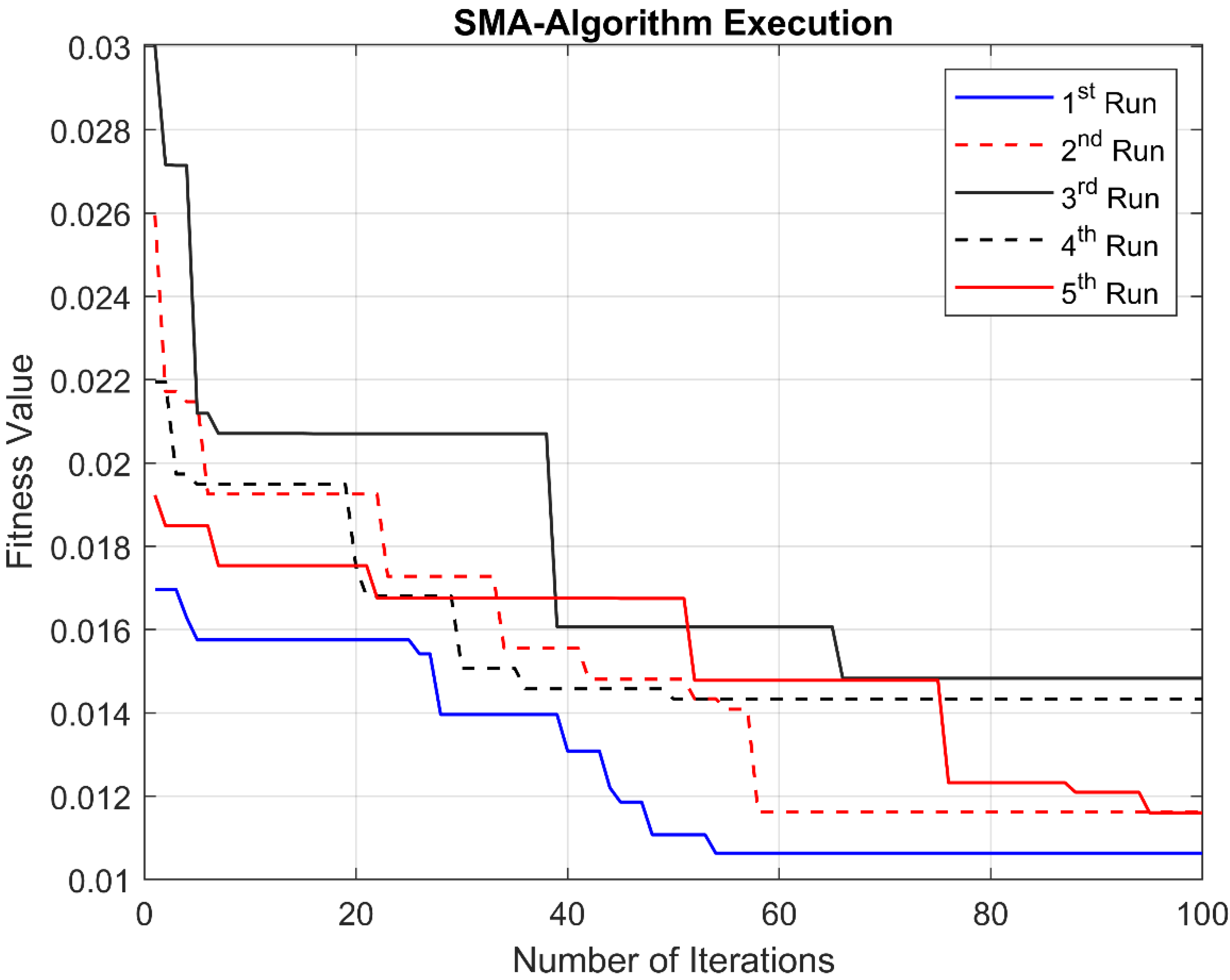To control the global/local optima results, the z-parameter was set to 0.05, which corresponds to the fifth iteration in Figure 2. In fact, there were various runs conducted, in each run, the value of the z-control parameter was changed to get the best global optima. For instance, in the first run in Figure 2, the z-parameter was 0.01, in the second run, z = 0.02, for the third run, z = 0.03, for the fourth run, z = 0.04. However, when the z-parameter was set to more than 0.05, the SMA fell into a prematurity problem. Hence, the z-parameter was fixed to 0.05, as listed in Table 2. With this value for the z-parameter, the algorithm was not premature, in other words, the algorithm tends to be global optima, as shown in Figure 2, where the curve continued to change its state near the end of the iterations.

On the other hand, the execution time was too long using a computer with 16 GB RAM and an Intel(R) Core(TM) i5-4200U CPU @ 1.60GHz 2.30 GHz processor in a 64-bit operating system. In each execution run, different features were obtained. However, the common features that are obtained in all of the five runs are “Service”, “src_bytes”, and “serror_rate”, where these features have been selected during four execution-runs, first, second, third, and fifth, as indicated in

Table 3. Selected Features Using SMA Runs.

Run No.	Obtained Features	Index of Feature in the Dataset
1	‘Service’	No. 3
	‘src_bytes’	No. 5
	‘hot’	No. 10
	‘serror_rate’	No. 25
	‘dst_host_srv_rerror_rate’	No. 41
2	‘Duration’	No. 1
	‘Service’	No. 3
	‘Flag’	No. 4
	‘src_bytes’	No. 5
	‘serror_rate’	No. 25
3	‘Service’	No. 3
	‘src_bytes’	No. 5
	‘dst_bytes’	No. 6
	‘serror_rate’	No. 25
	‘dst_host_srv_serror_rate’	No. 39
4	‘Duration’	No. 1
	‘Service’	No. 3
	‘Flag’	No. 4
	‘serror_rate’	No. 25
	‘dst_host_serror_rate’	No. 38
5	‘Service’	No. 3
	‘src_bytes’	No. 5
	‘Hot’	No. 10
	‘serror_rate’	No. 25
	‘dst_host_srv_serror_rate’	No. 39

. While in the fourth run, only “Service” and “src_bytes” appeared, besides other features. Furthermore, “hot” appeared in the first and last runs. Last but not least, the feature “dst_host_srv_serror_rate” was selected in the third and fifth runs. In other words, the most significant features are those indexed 3, 5, and 25 in the NSL-KDD dataset. Moreover, it is worth stating here that the SMA was not matured, as previously mentioned in Figure 2, and the algorithm was not biased to specific features, as listed in Table 3, where the selected attributes are varied from one execution run to another. The next significant features, which will be called lower-important features, are 10 and 39, hot and dst_host_srv_serror_rate, respectively. In the fifth execution run, all of the significant and lower-important features appeared, where this run was the best of the executions, as shown in Figure 2. It is shown that this run continued to change its status along the iterations, unlike the other curves in Figure 2.

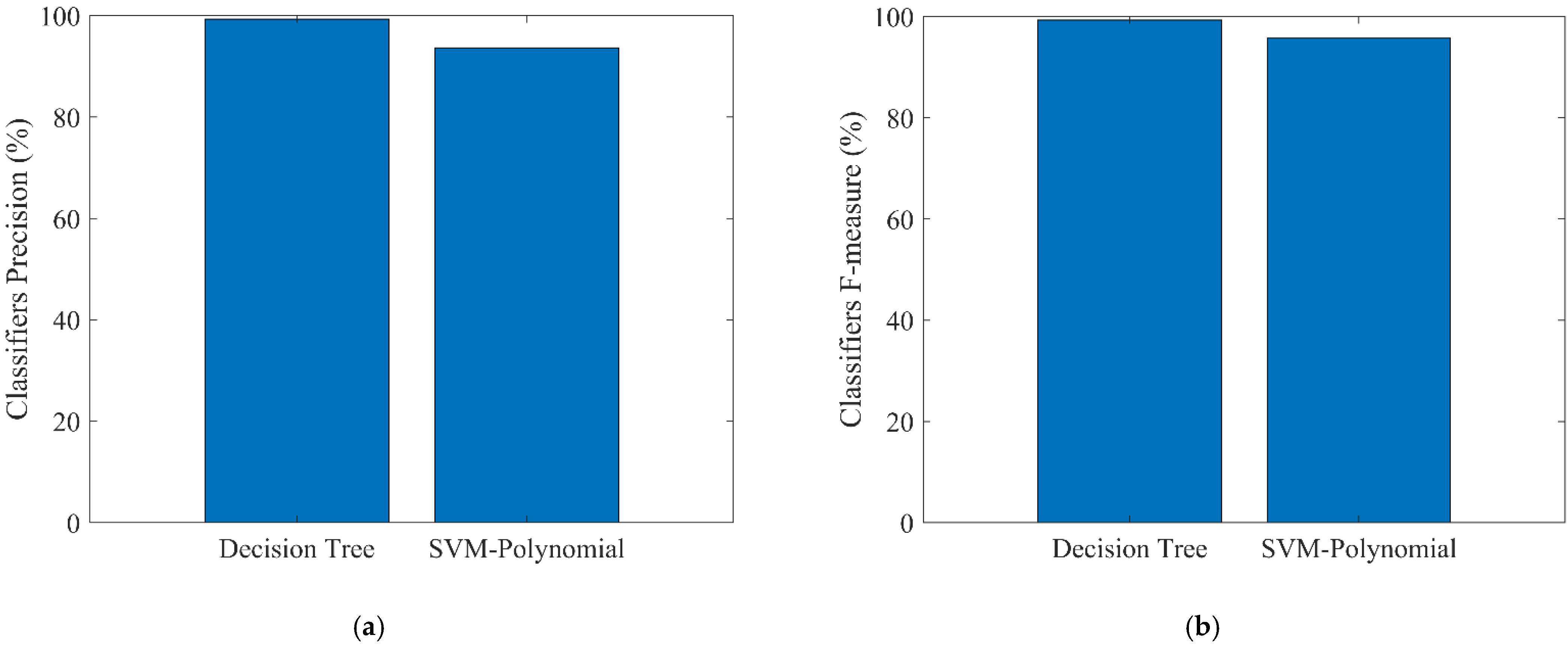
Consequently, the fifth execution-run has been adopted for the next step, which is the classification process using SVM with polynomial core and DT algorithms. Then, in this part, the binary classification will be achieved to detect the attack records using only five selected features, “Service”, “src_bytes”, “hot”, “serror_rate”, and “dst_host_srv_serror_rate”. In that way, Figure 3a shows the classification accuracy of the SVM polynomial and DT algorithms using only these five features. It can be seen that the classification accuracy of DT is 99.39% and 96.11% for the SVM polynomial algorithm. Both algorithms, DT and SVM polynomial, have shown good performance using the five features mentioned above. Although the accuracy of our proposed methodology is less than that obtained in [29], which was 99.73%, by 0.34% and 3.26% for the DT and SVM polynomial, respectively, but this was at the expense of the number of selected features. Where in [29], the number of selected features was 8, 11, and 13, while our approach was only five features.

In contrast, Figure 4 shows the FPR of these two algorithms. That is, the FPR was 0.54% and 5.33% for the DT and SVM polynomial algorithms, respectively. The FPR of the SVM polynomial algorithm was significantly more than that of the DT algorithm, where the DT algorithm’s FPR was less than 1%. In comparison to FPR, the TPR, or the sensitivity, is shown in Figure 3b. The DT sensitivity in Figure 3b was captured to be 99.36%, while SVM polynomial sensitivity was 97.89%. Our results for the sensitivity are almost close to those found in [29], but, as explained above, the expense was on the number of features. Note that when the number of features is increased, the training time and computational complexity, as well as the required memory, will be increased. That is, the sensitivity using the five-selected features was respectable. Thus, these five-features are full of information to be used in detecting attacks. Moreover, the accuracy of the RF-based feature selection in [37] was 95.21% and the FPR was 1.57% when the number of features equals 10. On the other hand, in [23], the best accuracy achieved using the bat algorithm was 96.42% with an FPR of 0.98%. However, the number of selected features was 32.

Table 4. Comparison of the proposed SMA with other research.

Technique		Number of Features	Accuracy
Our approach	DT	5	99.39%
	SVM		96.11%
Jaw and Wang [29]		Minimum of 8	99.73%
Li et al. [23]		32	96.42%
Li et al. [37]		10	95.21%

lists the comparison of our proposed approach with those in [23,29,37].

Figure 5 presents the specificity or the TNR for both the SVM polynomial and DT algorithms. The highest specificity achieved was 99.42%, delivered by the DT algorithm, while the other classifier gave 94.67%. That is, the same previous scenario, the DT algorithm outperforms the SVM polynomial algorithm. The overall error rate, on the other hand, is shown in Figure 6. As expected, the error rate of the DT algorithm outperformed that of the SVM polynomial algorithm. In that way, the error rates were 0.61% and 3.89% for each of the DT and SVM polynomial algorithms, respectively. Figure 7a shows the results of the precision of DT and SVM polynomial algorithms. The precision of the DT was 99.33% while the SVM polynomial produced 93.65%. The results in Figure 7a were expected since the previous results also showed that the DT algorithm outperformed SVM with the polynomial core algorithm. Last but not least, F-measure results are given in Figure 7b. As shown in the previous results, the DT continuously outperforms the SVM algorithm; that is, in Figure 7b, the DT also showed better performance than the SVM, where the F-measure of the DT algorithm was 99.34% and that of the SVM was 95.73%.

For the comparison of the classifiers’ performance measures, i.e., the DT and SVM performance measures, Figure 8 shows all of the above results in one place, for convenience. In other words, Figure 8 shows the accuracy, error rate, sensitivity, specificity, precision, false positive rate, and F-measure results of DT and SVM polynomial algorithms.

That is, from these results, it can be said that these five features, which were obtained from the feature reduction operation using the SMA, are certainly useful and full of information to almost detect most of the attackers. This can be confirmed in Figure 9. Thus, from Figure 9, the performance of the DT algorithm as compared with the SVM of polynomial core, is significantly outperforming. However, the errors shown in Figure 9, 0.9%, 3.0% for the SVM, and 0.3% (for both errors) for the DT algorithm, are comparable with those in other research. Although only five-features were used to deduce these results. Hence, the SMA for FS performed very well.

4. Conclusions

In this paper, the Slime Mould Algorithm (SMA) was suggested for feature reduction in a WSN intrusion detection system. The suggested algorithm reduced the number of features from 41 to five features only. The detection of attack records in the NSL-KDD dataset, which is an updated version of the KDD CUP 99 dataset, was performed using two algorithms, the SVM with polynomial core algorithm and the DT algorithm. The SMA showed a comparable performance with other research, where the confusion matrix measures showed significant results, in other words, the false positive rate, false negative rate, true positive rate, and true negative rate are improved significantly if contrasted with other works where only five features were selected using the SMA (“Service”, “src_bytes”, “Hot”, “serror_rate”, and “dst_host_srv_serror_rate”) and the measures were obtained based on these five features only. Thus, the accuracy was 99.39%, the error rate reached only 0.61%, the overall sensitivity was 99.36% when the specificity was 99.42%, while the FPR was reduced to 0.58%, and the F-measure was 99.34%. It is worth mentioning that the SMA may fall into a prematurity problem if not carefully set, in other words, the control parameters of the SMA should be selected properly before deploying it in the IDS. As a future development, implementing the presented methodology on different datasets and for multi-class categorization jobs is suggested.