Sampled-Data Linear Parameter Variable Approach for Voltage Regulation of DC–DC Buck Converter

Abstract

This paper addresses the new method for output voltage regulation of DC–DC buck converter nonlinear systems by a sampled-data linear parameter varying (LPV) controller. For this purpose, an output-error state-space affine LPV model is presented for DC–DC buck converter nonlinear systems. The sampled-data structure of the controller is considered as a time delay in the input, and stabilization conditions are obtained for LPV systems with affine dependence on the parameter by using a parameter-dependent Lyapunov–Krasovskii functional. Then, the design condition of the sampled-data LPV controller with an appropriate sampling period is derived to guarantee that the output voltage of the DC–DC buck converter can be adjusted to the desired voltage. Finally, simulation results are provided to show the validity of the presented approach in practical control applications where there are limitations on the value of the sampling period and the cost of the digital implementation.

1. Introduction

Power electronic systems play a crucial role in modern power systems by creating highly efficient interfaces as links between different sources, storage, and loads in DC networks [1]. In particular, DC–DC converters are often used in different stages of the network to handle regulated DC voltage and desired current to the units of the networks [2]. DC–DC converters utilized extensively in automotive electronics [3], renewable energy systems [4], hybrid energy storage system [5], satellite applications [6], and photovoltaic power applications [7].

A DC–DC converter should provide a fixed output voltage for the whole operating range, with load variations and non-constant power demand. Therefore, the closed-loop feedback control design for a DC–DC converter is important. The DC–DC buck converters (step-down) are one important structure of the converters that provide a lower output voltage than the input voltage. Because of the nonlinear characteristics of the DC–DC buck converter [8,9], it is of great importance that one use a nonlinear control approach in the problem of regulating the output voltage. A finite-time control method was presented for a nonlinear system, which was used for the DC–DC buck converter in [10]. By utilizing the backstepping approach, an adaptive nonlinear control method was proposed in [11], which obtained the output voltage regulation goal. A fuzzy self-regulating control method was employed in [12] for a DC–DC buck converter nonlinear system. In [13], a second-order control approach was proposed for a DC–DC buck converter by selecting the sliding surface appropriately. However, the proposed schemes are based on the presumption that the system states are available continuously in time and the controller output is applied immediately. However, in practice the system states are sampled periodically and the control signal has a delay for the computation.

With the development of programmable microcontroller technology, advanced nonlinear control approaches can be implemented with digital systems. A generalized proportional-integral controller for the DC–DC buck converter was implemented in the field-programmable gate array (FPGA), [14]. In [15], a type of fractional controller is designed for a DC–DC converter and implemented in a digital signal processor (DSP). In [16], a new approach based on the implicit discretization of the homogeneous differentiator to the digital controller design for a DC–DC buck converter with duty cycle saturation is presented. A digital fuzzy logic controller for the DC–DC buck converter is designed in [17], and the validity of the performance is evaluated with experimentation. A discrete-time sliding mode control of DC–DC converters is designed in [18], and the effectiveness of the controller is validated experimentally. Due to the complexity of the considering sampling period in the design of the controller, it is common to neglect this phenomenon and the sampling period for discrete-time controllers selected based on the engineering experience.

Sampled-data control methods, which can provide stable operation, have been extensively used for nonlinear systems over the past few years [19,20,21]. In [19], the global stabilization problem was presented, and the semi-global stabilization problem for the nonlinear systems was investigated in [21]. Recently, time-delay LPV systems have provided a suitable structure for sampled-data controller design for nonlinear systems [22,23]. The LPV method transforms the nonlinear model of the system into a simple parameter-variable linear model which is appropriate to design a time-varying controller for a nonlinear system. Inspired by the work [22,23,24] and considering the advantages of the LPV system [25] and the sampled-data control [26], we proposed a sampled-data LPV controller design method for a DC–DC buck converter nonlinear system to obtain robustness against load variations. In the first step, a new affine LPV model is derived, which describes the DC–DC buck converter nonlinear dynamics. Our objective is to design a sample-data LPV controller that achieved the output voltage regulation. To address this issue, the sampling rate of the states considered as the input delay and stability and stabilization conditions are derived for LPV systems with affine dependence on the parameter. We utilized the LKF approaches to derive design conditions that are appropriate for the stabilization and the sampled-data control of systems with time delay.

Due to the complexity of the considered sampling period in the design of the controller for the DC–DC buck converter, it is common to neglect this phenomenon, and the selection of the sampling period largely depends on the engineering experience, without theoretical support. If we want to improve the accuracy of the output voltage regulation, we usually decrease the sampling time in the cost of using the high-speed and expensive processor. However, if we want to increase the sampling period to reduce the cost of the implementation, the system performance may be decreased. Therefore, by using the LPV approach new theoretical results are provided, taking into account the nonlinear dynamics of the DC–DC buck converter and sampling and quantization of the measurements to a trade-off between the accuracy of the output voltage regulation and the sampling period.

The main contributions of this paper are as follows.

(i)

By using the LPV approach, new theoretical results are provided, taking into account the nonlinear dynamics of the DC–DC buck converter and sampling and quantization of the measurements.

(ii)

It is shown that the proposed LKF provides suitable bilinear matrix inequality conditions to compute the nonlinear control law by considering the sampling period which is suitable for practical control with low-cost digital implementation.

The rest of this paper is organized as follows. In Section 2, the nonlinear DC–DC buck converter model is presented, and then the LPV model is demonstrated. Section 3 is devoted to deriving stabilization conditions for sampled-data LPV controllers. The numerical simulation results and discussion about the controller performance are presented in Section 4.

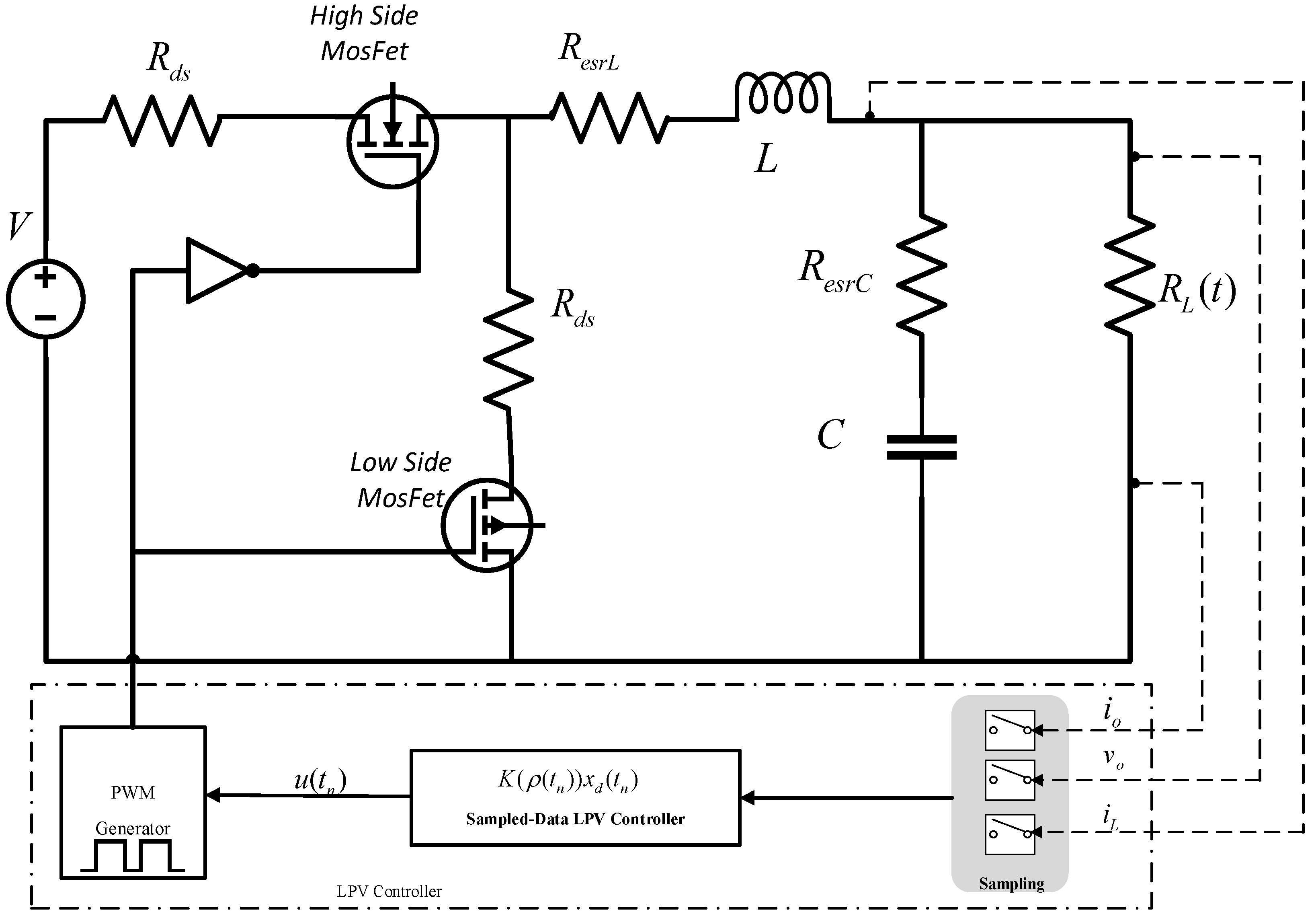
2. Problem Formulation and Preliminaries

The DC–DC buck power converter studied here with a sampled-data LPV controller is presented in Figure 1. The PWM control approach is utilized to obtain the output voltage regulation by controlling the semiconductor switches, whereas the duty ratio $\nu \left(t\right)\in \left[0,1\right]$ of PWM is adjusted by the digital controller. The DC–DC buck consists of a load resistance $R_L$, the static drain to source resistances of the power MOSFET $R_{DS}$, the circuit inductance L, the capacitance C, and equivalent series resistances of the inductor $R_{esrL}$ and capacitor $R_{esrC}$. V denotes the time-invariant input voltage. $v_o\left(t\right)$ and $i_L\left(t\right)$ define the output voltage and inductor current, respectively.

Figure 1. DC–DC buck converter topology with sampled-data LPV controller.

Sampled-data LPV controller changes the ratio of the duty cycle, $\nu \left(t\right)$ to control current and output voltage. Applying averaging method in [27], the mathematical nonlinear model of the DC–DC buck converter is as follows:

$$\begin{array}{c}\hfill {\dot{i}}_L\left(t\right)=-\frac{v_o\left(t\right)}{L}-\frac{R_{ds}+R_{esrL}}{L}{i}_L\left(t\right)+\frac{V\nu \left(t\right)}{L}\end{array}$$

(1)

$$\begin{array}{c}\hfill {\dot{v}}_C\left(t\right)=\frac{i_L\left(t\right)}{C}-\frac{1}{C{R}_L\left(t\right)}{v}_o\left(t\right)\end{array}$$

(2)

$$\begin{array}{c}\hfill {\dot{v}}_C\left(t\right)=\frac{1}{C{R}_{esrC}}\left(v_o\left(t\right)-v_c\left(t\right)\right).\end{array}$$

(3)

From (2) and (3), we get

$$\begin{array}{c}\hfill v_o\left(t\right)=\frac{R_L\left(t\right)}{R_L\left(t\right)+R_{esrC}}\left(R_{esrC}{i}_L\left(t\right)+v_c\left(t\right)\right).\end{array}$$

(4)

Considering $x_1\left(t\right)=i_L\left(t\right)$ and $x_2\left(t\right)=v_c\left(t\right)$, then (1) and (2) can be rewritten as follows:

$$\begin{array}{c}\hfill {\dot{x}}_1\left(t\right)=-\frac{1}{L}\left(\frac{R_L\left(t\right)R_{esrC}}{R_L\left(t\right)+R_{esrC}}+R_{ds}+R_{esrL}\right)x_1\left(t\right)-\frac{1}{L}\left(\frac{R_L\left(t\right)}{R_L\left(t\right)+R_{esrC}}\right)x_2\left(t\right)+\frac{V}{L}\nu \left(t\right)\end{array}$$

(5)

$$\begin{array}{c}\hfill {\dot{x}}_2\left(t\right)=\frac{1}{C}\left(\frac{R_L\left(t\right)}{R_L\left(t\right)+R_{esrC}}\right)x_1\left(t\right)-\frac{1}{C}\left(\frac{1}{R_L\left(t\right)+R_{esrC}}\right)x_2\left(t\right).\end{array}$$

(6)

Let ${\overline{x}}_2$ be an equilibrium point of $x_2\left(t\right)$. Then, by (6), the equilibrium point ${\overline{x}}_1$ is given by

$$\begin{array}{c}\hfill R_L\left(t\right){\overline{x}}_1-{\overline{x}}_2=0\to {\overline{x}}_1=\frac{{\overline{x}}_2}{R_L\left(t\right)}.\end{array}$$

(7)

Considering (3), the equilibrium point of $v_o\left(t\right)$ is given by ${\overline{v}}_o={\overline{x}}_2$. Thus, from (1), the equilibrium point of $\nu \left(t\right)$, we obtain

$$\begin{array}{c}\hfill \overline{\nu }=\frac{{\overline{x}}_2+\left(R_{ds}+R_{esrL}\right){\overline{x}}_1}{V}.\end{array}$$

(8)

In order to obtain the value of $v_c\left(t\right)$ from the measured $v_o\left(t\right),i_o\left(t\right)$ and $i_L\left(t\right)$, we used the following equality which was derived from (4). This is because measuring the value of $v_c\left(t\right)$ in the considered DC–DC buck converter is extremely hard. We have

$$\begin{array}{c}\hfill v_c\left(t\right)=v_o\left(t\right)+R_{esrC}(i_o\left(t\right)-i_L\left(t\right)).\end{array}$$

(9)

In the equilibrium point, from (9), $i_o=i_c$, because ${\overline{v}}_o={\overline{x}}_2$.

We can express the dynamics of the system based on the deviated state about the equilibrium point as follows:

$$\begin{array}{c}\hfill \left[\begin{array}{c}{x}_1\left(t\right)\hfill \\ x_2\left(t\right)\hfill \end{array}\right]=\left[\begin{array}{c}{x}_{1d}\left(t\right)\hfill \\ x_{2d}\left(t\right)\hfill \end{array}\right]+\left[\begin{array}{c}{\overline{x}}_1\hfill \\ {\overline{x}}_2.\hfill \end{array}\right]\end{array}$$

(10)

Equations (1) and (2) can be rewritten in terms of $x1d$, $x2d$ as follows:

$$\begin{array}{c}\hfill \begin{array}{c}{\dot{x}}_{1d}\left(t\right)=-\frac{1}{L}\left(\frac{R_L\left(t\right)R_{esrC}}{R_L\left(t\right)+R_{esrC}}+R_{ds}+R_{esrL}\right)x_{1d}\left(t\right)-\frac{1}{L}\left(\frac{R_L\left(t\right)}{R_L\left(t\right)+R_{esrC}}\right)x_{2d}\left(t\right)+\frac{V}{L}\nu \left(t\right)\hfill \\ -\frac{1}{L}\left(\frac{R_L\left(t\right)R_{esrC}}{R_L\left(t\right)+R_{esrC}}+R_{ds}+R_{esrL}\right){\overline{x}}_1-\frac{1}{L}\left(\frac{R_L\left(t\right)}{R_L\left(t\right)+R_{esrC}}\right){\overline{x}}_2\hfill \\ {\dot{x}}_{2d}\left(t\right)=\frac{1}{C}\left(\frac{R_L\left(t\right)}{R_L\left(t\right)+R_{esrC}}\right)x_{1d}\left(t\right)-\frac{1}{C}\left(\frac{1}{R_L\left(t\right)+R_{esrC}}\right)x_{2d}\left(t\right)\hfill \\ +\frac{1}{C}\left(\frac{R_L\left(t\right){\overline{x}}_1-{\overline{x}}_2}{R_L\left(t\right)+R_{esrC}}\right).\hfill \end{array}\end{array}$$

(11)

Because

$$\begin{array}{c}\hfill \frac{1}{V}\left(\frac{R_L\left(t\right)R_{esrC}}{R_L\left(t\right)+R_{esrC}}+R_{ds}+R_{esrL}\right){\overline{x}}_1+\frac{1}{V}\left(\frac{R_L\left(t\right)}{R_L\left(t\right)+R_{esrC}}\right){\overline{x}}_2=\frac{1}{V}\left({\overline{x}}_2+(R_{ds}+R_{esrL}){\overline{x}}_1\right)=\overline{\nu },\end{array}$$

(12)

when considering $u\left(t\right)=\nu \left(t\right)+\overline{\nu }$, the system given in (11) becomes

$$\begin{array}{c}\hfill \begin{array}{c}{\dot{x}}_{1d}\left(t\right)=-\frac{1}{L}\left(\frac{R_L\left(t\right)R_{esrC}}{R_L\left(t\right)+R_{esrC}}+R_{ds}+R_{esrL}\right)x_{1d}\left(t\right)-\frac{1}{L}\left(\frac{R_L\left(t\right)}{R_L\left(t\right)+R_{esrC}}\right)x_{2d}\left(t\right)+\frac{V}{L}u\left(t\right)\hfill \\ {\dot{x}}_{2d}\left(t\right)=\frac{1}{C}\left(\frac{R_L\left(t\right)}{R_L\left(t\right)+R_{esrC}}\right)x_{1d}\left(t\right)-\frac{1}{C}\left(\frac{1}{R_L\left(t\right)+R_{esrC}}\right)x_{2d}\left(t\right).\hfill \end{array}\end{array}$$

(13)

Let us define

$$\begin{array}{c}\hfill \rho \left(t\right)=\frac{1}{R_L\left(t\right)+R_{esrC}}.\end{array}$$

(14)

Then, we can rewrite (13) as follows:

$$\begin{array}{c}\hfill \begin{array}{c}{\dot{x}}_d\left(t\right)=A\left(\rho \left(t\right)\right)x_d\left(t\right)+Bu\left(t\right)\hfill \\ A\left(\rho \left(t\right)\right)=\left[\begin{array}{cc}-\frac{R_{esrC}-\rho R_{esrC}^2++R_{ds}+R_{esrL}}{L}& -\frac{1-\rho R_{esrC}}{L}\\ \frac{1-\rho R_{esrC}}{C}& \frac{-\rho R_{esrC}}{C}\end{array}\right],B=\left[\begin{array}{c}\frac{V}{L}\hfill \\ 0\hfill \end{array}\right].\hfill \end{array}\end{array}$$

(15)

Note that

$$\begin{array}{c}\hfill {\rho }_{min}=\frac{1}{R_{Up}+R_{esrC}}\le \rho \left(t\right)\le \frac{1}{R_{Low}+R_{esrC}}={\rho }_{max}.\end{array}$$

(16)

Therefore, we can derive the polytopic linear parameter varying (LPV) form of the DC–DC buck converter as follows:

$$\begin{array}{c}\hfill \begin{array}{c}{\dot{x}}_d\left(t\right)={\displaystyle \sum _{i=1}^2}{\alpha }_i{A}_i{x}_d\left(t\right)+Bu\left(t\right)\hfill \\ A_1=\left[\begin{array}{cc}-\frac{R_{esrC}-{\rho }_{max}{R}_{esrC}^2++R_{ds}+R_{esrL}}{L}& -\frac{1-{\rho }_{max}{R}_{esrC}}{L}\\ \frac{1-{\rho }_{max}{R}_{esrC}}{C}& \frac{-{\rho }_{max}{R}_{esrC}}{C}\end{array}\right]\hfill \\ A_2=\left[\begin{array}{cc}-\frac{R_{esrC}-{\rho }_{min}{R}_{esrC}^2++R_{ds}+R_{esrL}}{L}& -\frac{1-{\rho }_{min}{R}_{esrC}}{L}\\ \frac{1-{\rho }_{min}{R}_{esrC}}{C}& \frac{-{\rho }_{min}{R}_{esrC}}{C}\end{array}\right]\hfill \\ \alpha {}_1=\frac{\rho \left(t\right)-{\rho }_{min}}{{\rho }_{max}-{\rho }_{min}},\alpha {}_2=1-\alpha {}_1=\frac{{\rho }_{max}-\rho \left(t\right)}{{\rho }_{max}-{\rho }_{min}}\hfill \end{array}.\end{array}$$

(17)

The variation of the $R_L\left(t\right)$ can be established as follows:

$$\begin{array}{c}\hfill R_L\left(t\right)=\left\{\begin{array}{c}{R}^{Low}if\frac{v_o\left(t\right)}{i_o\left(t\right)}<R^{Low}\hfill \\ \frac{v_o\left(t\right)}{i_o\left(t\right)}Othervise\hfill \\ R^{Up}if\frac{v_o\left(t\right)}{i_o\left(t\right)}>R^{Up}\hfill \end{array}.\right.\end{array}$$

(18)

3. Problem Formulation

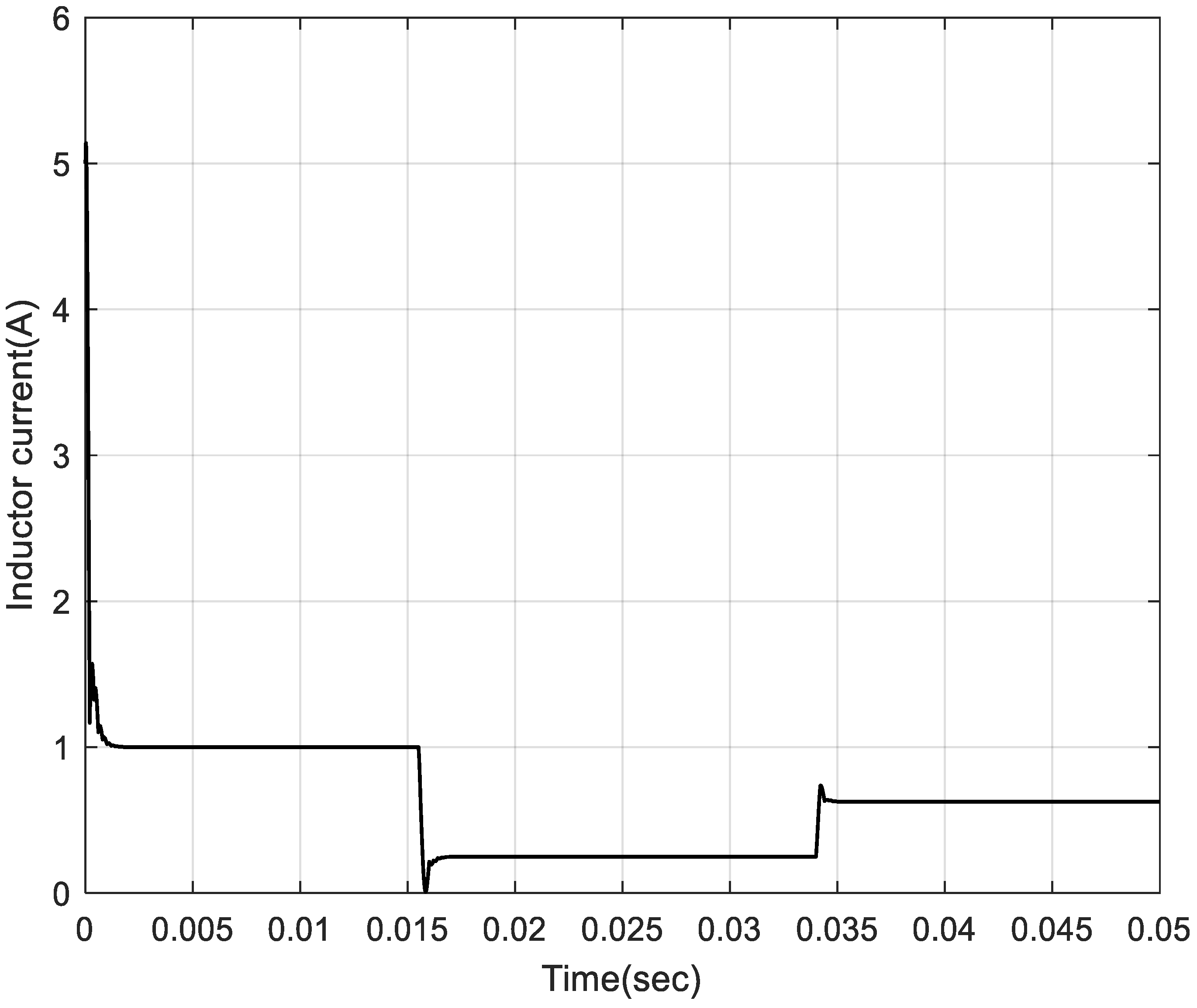
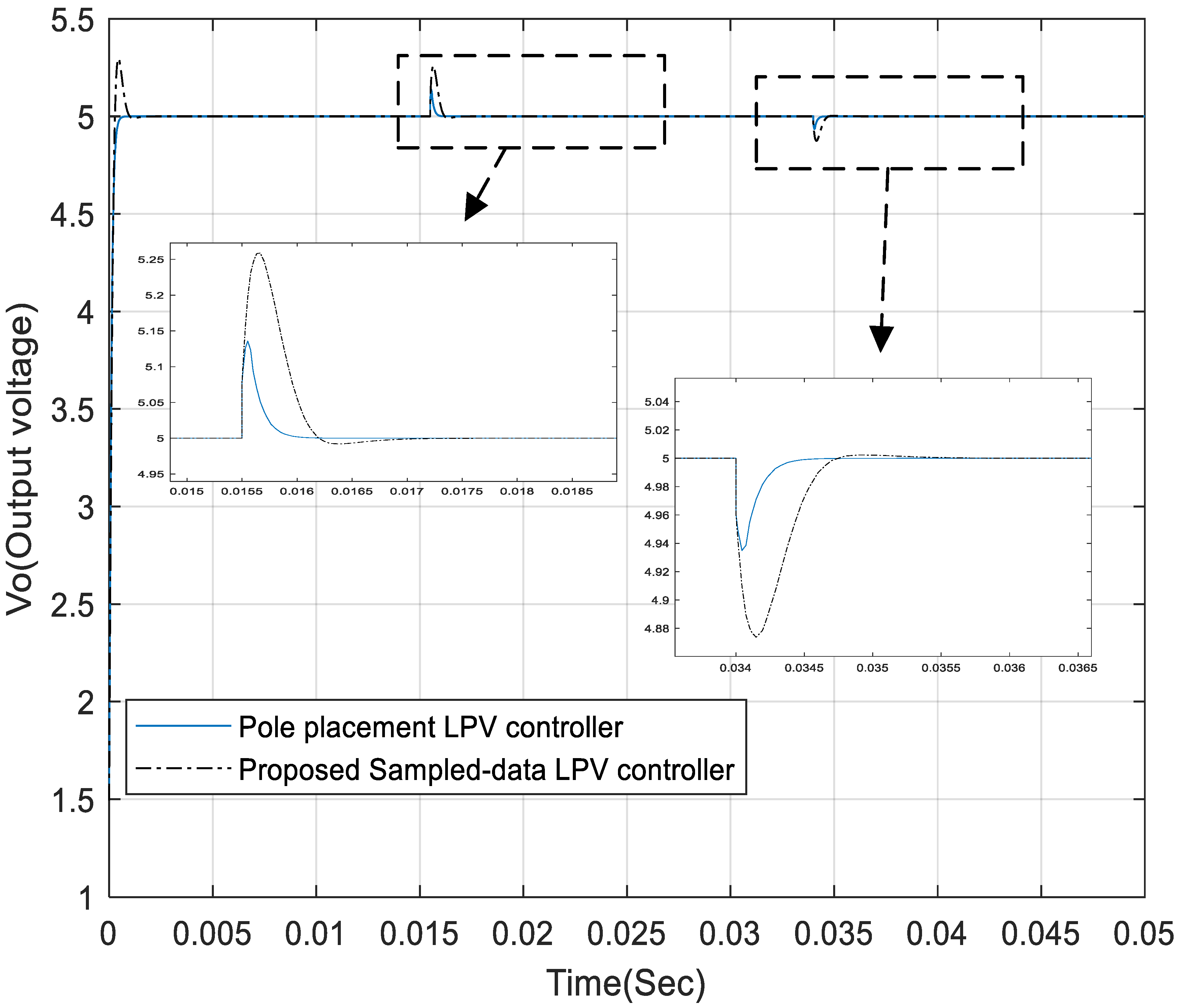
Sampled-data LPV controller in Figure 1 uses the system states measurement at sampling instants $t_n,n\in N$, needing

$$\begin{array}{c}\hfill 0<t_1<...<t_n<...,T_m=t_{n+1}-t_n,\end{array}$$

(19)

where $T_m$ shows the sampling period. Based on the measurement value of the state vector, the controller output is updated at each sampling instant; therefore, the control signal will be piecewise constant. We have

$$\begin{array}{c}\hfill u\left(t_n\right)=K\left(\rho \left(t_n\right)\right)x_d\left(t_n\right)t_n\le t<t_{n+1}.\end{array}$$

(20)

By utilizing the input delay approach, the sampled-data structure is modeled as a time-varying delay in the input which is defined by

$$\begin{array}{cc}\hfill & \tau \left(t\right)=t-t_{n}fort\in \left[t_n,t_{n+1}\right),n\in N.\hfill \end{array}$$

(21)

The function $\tau \left(t\right)$ is a sawtooth function which shows the time passed from the last sampling instant.

By substitution of Equation (20) into Equation (15), the following closed-loop system is obtained:

$$\begin{array}{c}\hfill \dot{x_d}\left(t\right)=A\left(\rho \left(t\right)\right)x_d\left(t\right)+BK\left(\rho (t-\tau \left(t\right))\right)x_d(t-\tau \left(t\right))\hfill \\ \hfill t_n\le t<t_{n+1}.\hfill \end{array}$$

(22)

Although $\rho \left(t\right)$ changes continuously in time, the $\rho \left(t_n\right)$ in the control law is kept constant between two samples. The difference among the $\rho \left(t\right)$ and the $\rho \left(t_n\right)$ depends on the rate of the parameter variation and the sampling period of the parameter. By using $\left|\dot{\rho }\left(t\right)\right|<v$ and applying the mean-value theorem, we have

$$\begin{array}{c}\hfill \left|\rho \left(t\right)-\rho \left(t_n\right)\right|<v\tau \left(t\right).\end{array}$$

(23)

Consequently,

$$\begin{array}{c}\hfill \rho \left(t\right)=\rho \left(t_n\right)+\mathrm{\Delta }\left(t\right),\left|\mathrm{\Delta }\left(t\right)\right|<v{T}_m.\end{array}$$

(24)

Because $\dot{\rho }\left(t\right)=\dot{\mathrm{\Delta }}\left(t\right)$ in the sampling interval, then

$$\begin{array}{c}\hfill -v\le \dot{\mathrm{\Delta }}\left(t\right)\le v.\end{array}$$

(25)

We should consider this uncertainty in the design conditions. By using (24), the open-loop system matrix depends on the uncertainty and the value of the measured parameter. Then we get

$$\begin{array}{c}\hfill {\dot{x}}_d\left(t\right)=A\left(\rho \left(t_n\right)+\mathrm{\Delta }\left(t\right)\right)x_d\left(t\right)+BK\left(\rho \left(t_n\right)\right)x_d(t-\tau \left(t\right)).\end{array}$$

(26)

In the following, conditions for the asymptotic stability of the closed-loop system in (26) were derived. We utilized the following lemmas in deriving the main results. In some cases, for the sake of simplicity, explicit dependence on t is omitted to shorten the notation.

Lemma 1

([28]). Consider a differentiable function $x\left(t\right)$ verifying

$$\begin{array}{c}\hfill {\int }_{t_n}^t\left[\begin{array}{c}\dot{x}\left(s\right)\\ x\left(t_n\right)\end{array}\right]ds=\left[\begin{array}{cc}I& -I\\ 0& \tau \left(t\right)I\end{array}\right]\left[\begin{array}{c}x\left(t\right)\hfill \\ x\left(t_n\right)\hfill \end{array}\right].\end{array}$$

(27)

For a real matrix $R\left(\rho \right)=R^T\left(\rho \right)>0$, there exists a matrix $N\left(\rho \right)$, such that the inequality

$$\begin{array}{c}\hfill -{\int }_{t_n}^t\left[\begin{array}{c}\dot{x}\left(s\right)\\ x\left(t_n\right)\end{array}\right]R\left(\rho \right)\left[\begin{array}{c}\dot{x}\left(s\right)\\ x\left(t_n\right)\end{array}\right]ds\le \left[\begin{array}{c}x\left(t\right)\hfill \\ x\left(t_n\right)\hfill \end{array}\right]\mathrm{\Theta }\left(\rho \right)\left[\begin{array}{c}x\left(t\right)\hfill \\ x\left(t_n\right)\hfill \end{array}\right]\end{array}$$

(28)

holds for all $x(.)$ and where

$$\begin{array}{c}\hfill \mathrm{\Theta }\left(\rho \right)=\left[\begin{array}{cc}I& -I\\ 0& \tau \left(t\right)I\end{array}\right]N\left(\rho \right)+\left[\begin{array}{cc}I& 0\\ -I& \tau \left(t\right)I\end{array}\right]N^T\left(\rho \right)+\tau \left(t\right)N\left(\rho \right)R^{-1}\left(\rho \right)N^T\left(\rho \right).\end{array}$$

(29)

Lemma 2

([22]). For a symmetric matrix O and two matrices M and L the following problem

$$\begin{array}{c}\hfill O+M^T\mathrm{\Theta }L+L^T{\mathrm{\Theta }}^{T}M<0\end{array}$$

(30)

is solvable if and only if

$$\begin{array}{c}\hfill M^{{\perp }^T}O{M}^{\perp }<0,L^{{\perp }^T}O{L}^{\perp }<0,\end{array}$$

(31)

where $M^{\perp }$ and $L^{\perp }$ denote arbitrary bases of the null spaces of M and L respectively, $M{M}^{\perp }=0$ and $L{L}^{\perp }=0$.

For the following parameter-dependent Lyapunov–Krasovskii functional

$$\begin{array}{c}\hfill \begin{array}{c}V\left(t\right)=x_d^T\left(t\right)P\left(\rho \left(t\right)\right)x_d\left(t\right)+(t_{n+1}-t)x_d^T\left(t_n\right)Q\left(\rho \left(t_n\right)\right)x_d\left(t_n\right)\hfill \\ +(t_{n+1}-t){\int }_{t_n}^t{\left[\begin{array}{c}{\dot{x}}_d\left(s\right)\\ x_d\left(t_n\right)\end{array}\right]}^T\left[\begin{array}{cc}{R}_1\left(\rho \left(t_n\right)\right)& R_2\left(\rho \left(t_n\right)\right)\\ *& R_3\left(\rho \left(t_n\right)\right)\end{array}\right]\left[\begin{array}{c}{\dot{x}}_d\left(s\right)\\ x_d\left(t_n\right)\end{array}\right]ds\hfill \end{array}\end{array}$$

(32)

with

$$\begin{array}{c}\hfill \begin{array}{c}P\left(\rho \left(t\right)\right)=P_1+(\rho \left(t_n\right)+\mathrm{\Delta }\left(t\right))P_2,Q\left(\rho \left(t_n\right)\right)=Q_1+\rho \left(t_n\right)Q_2\hfill \\ R_i\left(\rho \left(t_n\right)\right)=R_{i1}+\rho \left(t_n\right)R_{i2},i=1,2,3\hfill \end{array}.\end{array}$$

(33)

For $P\left(\rho \right)>0$, with the constraints on

$$\begin{array}{c}\hfill \left[\begin{array}{cc}{R}_1\left(\rho \left(t_n\right)\right)& R_2\left(\rho \left(t_n\right)\right)\\ *& R_3\left(\rho \left(t_n\right)\right)\end{array}\right]>0\end{array}$$

(34)

and

$$\begin{array}{c}\hfill \left[\begin{array}{cc}P\left(\rho \right(t\left)\right)& 0\\ 0& \left(T_m\right)Q\left(\rho \left(t_n\right)\right)\end{array}\right]>0,\end{array}$$

(35)

the LKF $V\left(t\right)$ is a positive definite function and there exists a small $\beta$ such that

$$\begin{array}{c}\hfill V\left(t\right)>\beta {∥x\left(t\right)∥}^2.\end{array}$$

(36)

Now, it is required to derive conditions that the LKF functional (32) is non-increasing at sampling instants $t=t_n$.

The first term of the LKF is continuous in time, so it is nonincreasing at sampling instants. The second and integral terms of the LKF have positive values due to (34) and (35) and are continuous on $(t_n,t_{n+1})$. At the sampling instants, we have $\underset{t\to t_{n+1}}{lim}(t_{n+1}-t)=0$, and they become zero; thus, we have ${\displaystyle \underset{t\to t_{n+1}}{lim}}V\left(t\right)=x^T\left(t_{n+1}\right)P\left(\rho \left(t_{n+1}\right)\right)x\left(t_{n+1}\right)$.

Therefore, the condition

$$\begin{array}{c}\hfill \underset{t\to t_{n+1}}{lim}V\left(t\right)\ge V\left(t_{n+1}\right)\end{array}$$

(37)

holds, and LKF (32) will be nonincreasing at sampling instants.

The derivative of $V\left(t\right)$ is given by

$$\begin{array}{c}\hfill \begin{array}{c}\dot{V}\left(t\right)={\dot{x}}_d^T\left(t\right)P\left(\rho \right)x_d\left(t\right)+x_d^T\left(t\right)P\left(\rho \right)\dot{x}\left(t\right)+x^T\left(t\right)\dot{P}\left(\rho \right)x\left(t\right)+\hfill \\ -x_d^T\left(t_n\right)Q\left(\rho \right)x_d\left(t\right)+\left(t_{n+1}-t\right)x_d^T\left(t_n\right)\dot{Q}\left(\rho \right)x_d\left(t\right)+\hfill \\ -{\int }_{t_n}^t{\left[\begin{array}{c}{\dot{x}}_d\left(s\right)\\ x_d\left(t_n\right)\end{array}\right]}^T\left[\begin{array}{cc}{R}_1\left(\rho \right)& R_2\left(\rho \right)\\ \ast & R_3\left(\rho \right)\end{array}\right]\left[\begin{array}{c}{\dot{x}}_d\left(s\right)\\ x_d\left(t_n\right)\end{array}\right]ds+\hfill \\ \left(t_{n+1}-t\right){\left[\begin{array}{c}{\dot{x}}_d\left(s\right)\\ x_d\left(t_n\right)\end{array}\right]}^T\left[\begin{array}{cc}{R}_1\left(\rho \right)& R_2\left(\rho \right)\\ \ast & R_3\left(\rho \right)\end{array}\right]\left[\begin{array}{c}{\dot{x}}_d\left(t\right)\\ x_d\left(t_n\right)\end{array}\right]\hfill \end{array}.\end{array}$$

(38)

Replacing (26) in (38) and applying Lemma 1 on the integral term of the LKF the upper bound of the derivative of $V\left(t\right)$ can be estimated as

$$\begin{array}{c}\hfill \dot{V}\left(t\right)\le {\left[\begin{array}{c}{x}_d\left(t\right)\\ x_d\left(t_n\right)\end{array}\right]}^T\left(\begin{array}{c}{\overline{\mathrm{\Lambda }}}_1\left(\rho \right)+(t_{n+1}-t){\overline{\mathrm{\Lambda }}}_2\left(\rho \right)+\tau \left(t\right){\overline{\mathrm{\Lambda }}}_3\left(\rho \right)+...\hfill \\ \tau \left(t\right)N\left(\rho \right)R{}^{-1}\left(\rho \right)N^T\left(\rho \right)\hfill \end{array}\right)\left[\begin{array}{c}{x}_d\left(t\right)\\ x_d\left(t_n\right)\end{array}\right]\end{array}$$

(39)

where

$$\begin{array}{c}\hfill \begin{array}{c}{\overline{\mathrm{\Lambda }}}_1\left(\rho \right)=\left[\begin{array}{cc}{\left(A^T\left(\rho \right)P\left(\rho \right)\right)}^H-N_{11}^H\left(\rho \right)+\dot{P}\left(\rho \right)& *\\ K^T\left(\rho \right)B^{T}P\left(\rho \right)+N_{11}^T\left(\rho \right)-N_{21}\left(\rho \right)& -Q\left(\rho \right)+N_{21}^H\left(\rho \right)\end{array}\right]\hfill \\ {\overline{\mathrm{\Lambda }}}_2\left(\rho \right)=\left[\begin{array}{cc}{A}^T\left(\rho \right)R_1\left(\rho \right)A\left(\rho \right)& A^T\left(\rho \right)R_1\left(\rho \right)BK\left(\rho \right)+A^T\left(\rho \right)R_2\left(\rho \right)\\ *& \overline{\mathrm{\Lambda }}\end{array}\right]\hfill \\ \overline{\mathrm{\Lambda }}=K^T\left(\rho \right)B^T{R}_1\left(\rho \right)BK\left(\rho \right)+\dot{Q}\left(\rho \right)+R_3\left(\rho \right)+{\left(R_2^T\left(\rho \right)BK\left(\rho \right)\right)}^H\hfill \\ {\overline{\mathrm{\Lambda }}}_3\left(\rho \right)=\left[\begin{array}{cc}0& N_{12}\left(\rho \right)\\ N_{12}^T\left(\rho \right)& N_{12}^T\left(\rho \right)+N_{12}\left(\rho \right)\end{array}\right]\hfill \end{array}.\end{array}$$

(40)

Because (39) is affine in t, then for $t=t_n$,

$$\begin{array}{c}\hfill {\overline{\mathrm{\Lambda }}}_1\left(\rho \right)+T_m{\overline{\mathrm{\Lambda }}}_2\left(\rho \right)<0\end{array}$$

(41)

and for $t=t_{n+1}$

$$\begin{array}{c}\hfill \left[\begin{array}{cc}{\overline{\mathrm{\Lambda }}}_1\left(\rho \right)+T_m{\overline{\mathrm{\Lambda }}}_3\left(\rho \right)& T_{m}N\left(\rho \right)\\ \ast & -T_{m}R\left(\rho \right)\end{array}\right]<0,\end{array}$$

(42)

implying that a small enough $\delta$ exists, so that the following is satisfied

$$\begin{array}{c}\hfill \dot{V}\left(t\right)<-\delta {∥x\left(t\right)∥}^2.\end{array}$$

(43)

Thus the closed-loop system (26) with a time delay of less than $T_m$, is asymptotically stable.

Derived conditions for stability in (41) and (42) are polynomially parameter-dependent matrix inequalities, because of the product of the system matrix $A\left(\rho \right)$ with $P\left(\rho \right)$ and $R_1\left(\rho \right)$. These conditions should be satisfied for all parameter space $\rho \left(t\right)$. Therefore, these conditions are not suitable for sampled-data LPV controller design purposes because they require an infinite number of constraints to be checked. In the following, these conditions are transformed to new stability conditions by using the Lemma 2, which is helpful for convexification purposes.

Theorem 1.

Closed-loop system (26) with a time delay less than $T_m$ is asymptotically stable if there exist matrix functions $P\left(\rho \right)\in S^n>0$, $Q\left(\rho \right)$, $R_1\left(\rho \right)$, $R_2\left(\rho \right)\in S^n$, $R_3\left(\rho \right)$, $N_{11}\left(\rho \right)$, $N_{12}\left(\rho \right)$, $N_{21}\left(\rho \right)$, $N_{22}\left(\rho \right)$, ${{\rm Y}}_1$, ${{\rm Y}}_2$, ${{\rm Y}}_3$, ${{\rm Y}}_4$, ${{\rm Y}}_5$, ${{\rm Y}}_6$$\in R^{n\times n}$ and controller $K\left(\rho \right)$, such that for all ρ the parameterized matrix inequalities problems (44)–(47) are feasible. We have

$$\begin{array}{l}\left[\begin{array}{cc}{R}_1\left(\rho \right)& R_2\left(\rho \right)\\ *& R_3\left(\rho \right)\end{array}\right]>0\hfill \end{array}$$

(44)

$$\begin{array}{l}\left[\begin{array}{cc}P\left(\rho \right)& 0\\ *& T_{m}Q\left(\rho \right)\end{array}\right]>0\hfill \end{array}$$

(45)

$$\begin{array}{l}\left[\begin{array}{ccc}{T}_m{R}_1\left(\rho \right)-{{{\rm Y}}_1}^H& {\mathrm{\Lambda }}_1\left(\rho \right)& {\mathrm{\Lambda }}_2\left(\rho \right)+{\mathrm{\Lambda }}_3\left(\rho \right)\\ *& {\mathrm{\Lambda }}_4\left(\rho \right)+{\mathrm{\Lambda }}_5\left(\rho \right)& {\mathrm{\Lambda }}_6\left(\rho \right)+{\mathrm{\Lambda }}_7\left(\rho \right)\\ *& *& {\mathrm{\Lambda }}_8\left(\rho \right)+{\mathrm{\Lambda }}_9\left(\rho \right)\end{array}\right]<0\hfill \end{array}$$

(46)

$$\begin{array}{l}\left[\begin{array}{ccccc}-{{{\rm Y}}_4}^H& {\mathrm{\Lambda }}_{10}\left(\rho \right)& {{\rm Y}}_4^{T}BK\left(\rho \right)C-{{\rm Y}}_6& 0& 0\\ *& {\mathrm{\Lambda }}_{11}\left(\rho \right)& {\mathrm{\Lambda }}_{12}\left(\rho \right)& T_m{N}_{11}\left(\rho \right)& T_m{N}_{12}\left(\rho \right)\\ *& *& {\mathrm{\Lambda }}_{13}\left(\rho \right)& T_m{N}_{21}\left(\rho \right)& T_m{N}_{22}\left(\rho \right)\\ *& *& *& -T_m{R}_1\left(\rho \right)& -T_m{R}_2\left(\rho \right)\\ *& *& *& *& -T_m{R}_3\left(\rho \right)\end{array}\right]<0\hfill \end{array}$$

(47)

where

$$\begin{array}{c}\hfill \begin{array}{c}{\mathrm{\Lambda }}_1\left(\rho \right)=P\left(\rho \right)+{{\rm Y}}_1^{T}A\left(\rho \right)-{{\rm Y}}_2\hfill \\ {\mathrm{\Lambda }}_2\left(\rho \right)=T_m{R}_2\left(\rho \right)\hfill \\ {\mathrm{\Lambda }}_3\left(\rho \right)=-{{\rm Y}}_3+{{\rm Y}}_1^{T}BK\left(\rho \right)\hfill \\ {\mathrm{\Lambda }}_4\left(\rho \right)=\dot{P}\left(\rho \right)-Q\left(\rho \right)-N_{11}{\left(\rho \right)}^H\hfill \\ {\mathrm{\Lambda }}_5\left(\rho \right)={\left(A^T\left(\rho \right){{\rm Y}}_2\right)}^H\hfill \\ {\mathrm{\Lambda }}_6\left(\rho \right)=N_{11}\left(\rho \right)-N_{21}^T\left(\rho \right)\hfill \\ {\mathrm{\Lambda }}_7\left(\rho \right)={{\rm Y}}_2^{T}BK\left(\rho \right)+A^T\left(\rho \right){{\rm Y}}_3\hfill \\ {\mathrm{\Lambda }}_8\left(\rho \right)=N_{21}{\left(\rho \right)}^H-Q\left(\rho \right)\hfill \\ {\mathrm{\Lambda }}_9\left(\rho \right)={\left({{\rm Y}}_3^{T}BK\left(\rho \right)\right)}^H+T_m\dot{Q}\left(\rho \right)+T_m{R}_3\left(\rho \right)\hfill \\ {\mathrm{\Lambda }}_{10}\left(\rho \right)=P\left(\rho \right)-{{\rm Y}}_5+{{\rm Y}}_4^{T}A\left(\rho \right)\hfill \\ {\mathrm{\Lambda }}_{11}\left(\rho \right)=\dot{P}\left(\rho \right)-N_{11}{\left(\rho \right)}^H+{\left({{\rm Y}}_5^{T}A\left(\rho \right)\right)}^H\hfill \\ {\mathrm{\Lambda }}_{12}\left(\rho \right)={\mathrm{\Lambda }}_6\left(\rho \right)+A^T\left(\rho \right){{\rm Y}}_6-T_m{N}_{12}\left(\rho \right)+{{\rm Y}}_5^{T}BK\left(\rho \right)\hfill \\ {\mathrm{\Lambda }}_{13}\left(\rho \right)={\mathrm{\Lambda }}_8\left(\rho \right)-T_m{N}_{22}{\left(\rho \right)}^H+{\left({{\rm Y}}_6^{T}BK\left(\rho \right)\right)}^H.\hfill \end{array}\end{array}$$

Proof. 

The matrix inequalities in (44) and (45), which are taken from (34) and (35) are sufficient conditions for the positiveness of the LKF $V\left(t\right)$. The matrix inequalities in (46) and (47) are derived respectively from (41) and (42), which are sufficient conditions for the negativeness of the derivative of LKF $V\left(t\right)$. To prove this issue, we rewrite (46) as

$$\begin{array}{c}\hfill O_1(\rho ,\dot{\rho })+M_1^T\left(\rho \right){\mathrm{\Theta }}_1{L}_1+L_1^T{{\mathrm{\Theta }}_1}^T{M}_1\left(\rho \right)<0\end{array}$$

(48)

with

$$\begin{array}{c}\hfill \begin{array}{c}{O}_1(\rho ,\dot{\rho })=\left[\begin{array}{ccc}{T}_m{R}_1\left(\rho \right)& P\left(\rho \right)& {\mathrm{\Lambda }}_2\left(\rho \right)\\ *& {\mathrm{\Lambda }}_4\left(\rho \right)& {\mathrm{\Lambda }}_6\left(\rho \right)\\ *& *& {\mathrm{\Lambda }}_8\left(\rho \right)+T_m\dot{Q}\left(\rho \right)+T_m{R}_3\left(\rho \right)\end{array}\right]\hfill \\ M_1\left(\rho \right)=\left[-IA\left(\rho \right)BK\left(\rho \right)\right]\hfill \\ L_1=\left[\begin{array}{ccc}I& 0& 0\\ 0& 0& I\end{array}\right]\hfill \\ {\mathrm{\Theta }}_1=\left[\begin{array}{ccc}{{\rm Y}}_1& {{\rm Y}}_2& {{\rm Y}}_3\end{array}\right]\hfill \end{array}\end{array}$$

(49)

and rewrite (47) as

$$\begin{array}{c}\hfill O_2(\rho ,\dot{\rho })+M_2^T\left(\rho \right){\mathrm{\Theta }}_2{L}_2+L_2^T{{\mathrm{\Theta }}_2}^T{M}_2\left(\rho \right)<0\end{array}$$

(50)

with

$$\begin{array}{c}\hfill \begin{array}{c}{O}_2\left(\rho \right)=\left[\begin{array}{ccccc}0& P\left(\rho \right)& 0& 0& 0\\ *& \dot{P}\left(\rho \right)-N_{11}^H\left(\rho \right)& {\mathrm{\Lambda }}_6\left(\rho \right)-T_m{N}_{12}\left(\rho \right)& T_m{N}_{11}\left(\rho \right)& T_m{N}_{12}\left(\rho \right)\\ *& *& {\mathrm{\Lambda }}_8\left(\rho \right)-T_m{N}_{22}^H\left(\rho \right)& T_m{N}_{21}\left(\rho \right)& T_m{N}_{22}\left(\rho \right)\\ *& *& *& -T_m{R}_1\left(\rho \right)& -T_m{R}_2\left(\rho \right)\\ *& *& *& *& -T_m{R}_3\left(\rho \right)\end{array}\right]\hfill \\ M_2\left(\rho \right)=\left[-IA\left(\rho \right)BK\left(\rho \right)00\right]\hfill \\ L_2=\left[\begin{array}{ccccc}I& 0& 0& 0& 0\\ 0& I& 0& 0& 0\\ 0& 0& I& 0& 0\end{array}\right]\hfill \\ {\mathrm{\Theta }}_2=\left[\begin{array}{ccc}{{\rm Y}}_4& {{\rm Y}}_5& {{\rm Y}}_6\end{array}\right]\hfill \end{array}.\end{array}$$

(51)

By defining $M_1\left(\rho \right)$ and $M_2\left(\rho \right)$ as

$$\begin{array}{c}\hfill \begin{array}{c}{M}_1^{\perp }\left(\rho \right)=\left[\begin{array}{cc}A\left(\rho \right)& BK\left(\rho \right)\\ I& 0\\ 0& I\end{array}\right]\hfill \\ M_2^{\perp }\left(\rho \right)=\left[\begin{array}{cccc}A\left(\rho \right)& BK\left(\rho \right)& 0& 0\\ I& 0& 0& 0\\ 0& I& 0& 0\\ 0& 0& I& 0\\ 0& 0& 0& I\end{array}\right]\hfill \end{array},\end{array}$$

(52)

and utilizing Lemma 2, we reach the matrix inequalities in (41) and (42). Thus, the feasibility of (46) and (47) imply the feasibility of (41) and (42) respectively. The matrix variables ${{\rm Y}}_1$, ${{\rm Y}}_2$, ${{\rm Y}}_3$, ${{\rm Y}}_4$, ${{\rm Y}}_5$ and ${{\rm Y}}_6$ are the slack variables. This concludes the proof.

Remark 1.

If the matrices ${{\rm Y}}_i,i=1,\dots ,6$ chosen are parameter-independent, the conditions in Theorem 1 have affine dependence to the parameter. Therefore to ensure stability over the entire parameter space, the stability conditions in Theorem 1 should be solved at the vertices of the parameter value. When $K\left(\rho \right)$ is unknown, the matrix inequalities (46) and (47) are non-convex bilinear matrix inequality (BMI) optimization problems, and cannot be resolved by using the convex optimisation algorithm.

Remark 2.

PENBMI [29], is a intense software for solving the BMI problems. The algorithm used in PENBMI is based on the augmented Lagrangian method. It can be viewed as a generalization to nonlinear semidefinite problems of the penalty-barrier-multiplier method. Convergence to a critical point satisfying the first-order Karush–Kuhn–Tucker (KKT) optimality conditions is guaranteed. In this paper, we utilized PENBMI 2.0 interfaced with YALMIP 3.0 to solve the matrix inequalities in Theorem 1 and design a sampled-data output feedback LPV controller.

4. Simulation Study

We simulate the DC–DC buck converter by using the nonlinear model in (1)–(3) in MATLAB/Simulink software with the parameters that are listed in Table 1. As presented in Table 1, the equilibrium point of $v_c\left(t\right)=5$ is given by $v_c=5$, and the lower and upper bounds of $R_L\left(t\right)$ are given by $R^{Low}=2$ and $R^{Up}=25$.

Table 1. Parameters of the DC–DC Buck converter.

Parameters	Value
V (input power source)	12 V
${\overline{v}}_c$ (Equilibrium point of $v_c\left(t\right)$)	5 V
L	47  $\mathsf{\mu }$H
C	220 $\mathsf{\mu }$F
$R_{ds}$	30 m$\mathrm{\Omega }$
$R_{esrL}$	100 m$\mathrm{\Omega }$
$R_{esrC}$	110 m$\mathrm{\Omega }$
$R_L\left(t\right)$	5–25 $\mathrm{\Omega }$
Switching frequency	200 kHz

We applied PENBMI to solve Theorem 1 conditions with the sampling period chosen as T = 0.0005 s, and the following control law was obtained:

$$\begin{array}{c}\hfill u\left(t_n\right)=[-0.03200.0117]+[0.0003-0.0018]\rho \left(t_n\right).\end{array}$$

(53)

In the simulations, the proposed sampled-data LPV controller is implemented digitally by employing an analog-to-digital sampler and a zero-order hold. When the switching frequency is 200 kHZ, the simulation results for T = 0.0005 s are presented in Figure 2, Figure 3 and Figure 4 where the constant load changes from 5 $\mathrm{\Omega }$ to 20 $\mathrm{\Omega }$ and then back to 8 $\mathrm{\Omega }$. We compared the proposed sampled-data feedback LPV controller with a regional pole placement LPV technique [30]. Simulation results show that under the duty ratio function shown in Figure 3, the output voltage reaches faster to the steady value, and suitable performance is obtained by the proposed sampled-data feedback LPV controller than the pole placement LPV.

Figure 2. Comparison between output voltage regulation about the equilibrium point under the proposed controller (T = 0.0005 s) where the load is changed.

Figure 3. Manipulated duty cycle of the buck converter for embedded PWM control duty ratio in the presence of load variations (T = 0.0005 s).

Figure 4. Inductance current responses where the load is changed.

We repeated the simulation for T = 0.0002 s and the switching frequency 200 kHZ. Figure 5 shows that the output voltage $v_o$ adjusted to be steady in a shorter time by the pole placement with high-cost digital platforms. Consequently, it is crucial to select the suitable sampling period. If we want to modify the accuracy of the output voltage adjustment about the equilibrium point, we should decrease the sampling period. However, if we want to increase the sampling period to reduce the implementation cost, the system performance may be lost. The simulation results show the effectiveness of the proposed approach to reduce the implementation cost.

Figure 5. Comparison between output voltage response curves under the proposed controller (T = 0.0002 s) where the load is changed.

5. Conclusions

This paper presents a new sampled-data LPV controller for a DC–DC buck converter. The main advantages of this control scheme are the consideration of the nonlinear systems of the DC–DC buck converter and the sampling period in the design conditions. It has been proven that the regulation problem can be solved by choosing the sampling period appropriately. This feature is desirable for practical control applications where hardware resources and digital processing capabilities are limited. A simulation study shows a satisfactory performance of the proposed sampled-data LPV controller. For future works, we will experimentally verify the effectiveness of the proposed approach and extend the proposed approach for output feedback controllers in the presence of disturbances.

References

1. Yang, Y.; Wang, H.; Sangwongwanich, A.; Blaabjerg, F. Design for reliability of power electronic systems. In Power Electronics Handbook; Butterworth-Heinemann: Oxford, UK, 2018; pp. 1423–1440. [Google Scholar]
2. Goyal, V.K.; Shukla, A. Isolated DC-DC Boost Converter for Wide Input Voltage Range and Wide Load Range Applications. IEEE Trans. Ind. Electron. 2020, 68, 9527–9539. [Google Scholar] [CrossRef]
3. Park, J.; Choi, S. Design and control of a bidirectional resonant DC-DC converter for automotive engine/battery hybrid power generators. IEEE Trans. Power Electron. 2013, 29, 3748–3757. [Google Scholar] [CrossRef]
4. Xu, Q.; Zhang, C.; Wen, C.; Wang, P. A novel composite nonlinear controller for stabilization of constant power load in DC microgrid. IEEE Trans. Smart Grid 2017, 10, 752–761. [Google Scholar] [CrossRef]
5. Xu, Q.; Hu, X.; Wang, P.; Xiao, J.; Tu, P.; Wen, C.; Lee, M.Y. A decentralized dynamic power sharing strategy for hybrid energy storage system in autonomous DC microgrid. IEEE Trans. Ind. Electron. 2016, 64, 5930–5941. [Google Scholar] [CrossRef]
6. Naayagi, R.T.; Forsyth, A.J.; Shuttleworth, R. High-power bidirectional DC-DC converter for aerospace applications. IEEE Trans. Power Electron. 2012, 27, 4366–4379. [Google Scholar] [CrossRef]
7. Olalla, C.; Clement, D.; Rodriguez, M.; Maksimovic, D. Architectures and control of submodule integrated DC-DC converters for photovoltaic applications. IEEE Trans. Power Electron. 2012, 28, 2980–2997. [Google Scholar] [CrossRef]
8. Qiu, Y.; Chen, X.; Zhong, C.; Qi, C. Limiting integral loop digital control for DC-DC converters subject to changes in load current and source voltage. IEEE Trans. Ind. Inform. 2014, 10, 1307–1316. [Google Scholar]
9. Shi, L.F.; Jia, W.G. Mode-selectable high-efficiency low-quiescent-current synchronous buck DC-DC converter. IEEE Trans. Ind. Electron. 2013, 61, 2278–2285. [Google Scholar] [CrossRef]
10. Du, H.; Cheng, Y.; He, Y.; Jia, R. Finite-time output feedback control for a class of second-order nonlinear systems with application to DC-DC buck converters. Nonlinear Dyn. 2014, 78, 2021–2030. [Google Scholar] [CrossRef]
11. Salimi, M.; Soltani, J.; Markadeh, G.A.; Abjadi, N.R. Indirect output voltage regulation of DC-DC buck/boost converter operating in continuous and discontinuous conduction modes using adaptive backstepping approach. IET Power Electron. 2013, 6, 732–741. [Google Scholar] [CrossRef] [Green Version]
12. Li, Z.; Zhao, J. Output feedback stabilization for a general class of nonlinear systems via sampleddata control. Int. J. Robust Nonlinear Control. 2018, 28, 2853–2867. [Google Scholar] [CrossRef]
13. Ling, R.; Maksimovic, D.; Leyva, R. Second-order sliding-mode controlled synchronous buck DC-DC converter. IEEE Trans. Power Electron. 2015, 31, 2539–2549. [Google Scholar] [CrossRef]
14. Zurita-Bustamante, E.W.; Linares-Flores, J.; Guzmán-Ramírez, E.; Sira-Ramírez, H. A comparison between the GPI and PID controllers for the stabilization of a DC-DC “buck” converter: A field programmable gate array implementation. IEEE Trans. Ind. Electron. 2011, 58, 5251–5262. [Google Scholar] [CrossRef]
15. Seo, S.W.; Choi, H.H. Digital implementation of fractional order PID-type controller for boost DC-DC converter. IEEE Access 2019, 7, 142652–142662. [Google Scholar] [CrossRef]
16. Alarcon-Carbajal, M.A.; Carvajal-Rubio, J.E.; Sanchez-Torres, J.D.; Castro-Palazuelos, D.E.; Rubio-Astorga, G.J. An Output Feedback Discrete-Time Controller for the DC-DC Buck Converter. Energies 2022, 15, 528. [Google Scholar] [CrossRef]
17. Seguel, J.L.; Seleme, S.I., Jr. Robust Digital Control Strategy Based on Fuzzy Logic for a Solar Charger of VRLA Batteries. Energies 2021, 14, 1001. [Google Scholar] [CrossRef]
18. Ni, Y.; Xu, J. Study of discrete global-sliding mode control for switching DC-DC converter. J. Circuits Syst. Comput. 2011, 20, 1197–1209. [Google Scholar] [CrossRef]
19. Qian, C.; Du, H. Global output feedback stabilization of a class of nonlinear systems via linear sampled data control. IEEE Trans. Autom. Control 2012, 57, 2934–2939. [Google Scholar] [CrossRef]
20. Chu, H.; Qian, C.; Yang, J.; Xu, S.; Liu, Y. Almost disturbance decoupling for a class of nonlinear systems via sampled data output feedback control. Int. J. Robust Nonlinear Control 2016, 26, 2201–2215. [Google Scholar] [CrossRef]
21. Zhang, C.; Jia, R.; Qian, C.; Li, S. Semi global stabilization via linear sampled data output feedback for a class of uncertain nonlinear systems. Int. J. Robust Nonlinear Control 2015, 25, 2041–2061. [Google Scholar] [CrossRef]
22. Hooshm, K.; Bayat, F.; Jahed-Motlagh, M.R.; Jalali, A. Robust sampled data control of nonlinear LPV systems: Time dependent functional approach. IET Control Theory Appl. 2018, 12, 1318–1331. [Google Scholar] [CrossRef]
23. Hooshm, K.; Bayat, F.; Jahedmotlagh, M.; Jalali, A. Guaranteed cost nonlinear sampled data control: Applications to a class of chaotic systems. Nonlinear Dyn. 2020, 100, 731–748. [Google Scholar] [CrossRef]
24. Hooshm, K.; Bayat, F.; Jahed-Motlagh, M.R.; Jalali, A.A. Polynomial LPV approach to robust H control of nonlinear sampled-data systems. Int. J. Control 2020, 93, 2145–2160. [Google Scholar] [CrossRef]
25. Hoffmann, C.; Werner, H. A survey of linear parameter-varying control applications validated by experiments or high-fidelity simulations. IEEE Trans. Control Syst. Technol. 2014, 23, 416–433. [Google Scholar] [CrossRef]
26. Hetel, L.; Fiter, C.; Omran, H.; Seuret, A.; Fridman, E.; Richard, J.P.; Niculescu, S.I. Recent developments on the stability of systems with aperiodic sampling: An overview. Automatica 2017, 76, 309–333. [Google Scholar] [CrossRef] [Green Version]
27. Sun, J.; Grotstollen, H. Averaged modelling of switching power converters: Reformulation and theoretical basis. In Proceedings of the 23rd Annual IEEE Power Electronics Specialists Conference, Toledo, Spain, 29 June–3 July 1992; pp. 1165–1172. [Google Scholar]
28. Briat, C. Convergence and equivalence results for the Jensen’s inequality—Application to time-delay and sampled-data systems. IEEE Trans. Autom. Control 2011, 56, 1660–1665. [Google Scholar] [CrossRef] [Green Version]
29. Kocvara, M.; Stingl, M.; PENOPT GbR. PENBMI User’s Guide (Version 2.0); Software Manual, Hauptstrasse A; PENOPT GbR: Igensdorf, Germany, 2005; Volume 31, p. 91338. [Google Scholar]
30. Joo, H.; Kim, S.H. LPV control with pole placement constraints for synchronous buck converters with piecewise-constant loads. Math. Probl. Eng. 2015, 2015, 686857. [Google Scholar] [CrossRef]