Adversarial Image Colorization Method Based on Semantic Optimization and Edge Preservation

Abstract

As a medium for transmitting visual information, image is a direct reflection of the objective existence of the natural world. Grayscale images lack more visual information than color images. Therefore, it is of great significance to study the colorization of grayscale images. At present, the problems of semantic ambiguity, boundary overflow and lack of color saturation exist in both traditional and deep learning methods. To solve the above problems, an adversarial image colorization method based on semantic optimization and edge preservation is proposed. By improving generative and discriminative networks and designing loss functions, deeper semantic information and sharper edges of images can be learned by our network. Our experiments are carried out on the public datasets Place365 and ImageNet. The experimental results show that the method in this paper can reduce the color anomaly caused by semantic ambiguity, suppress the color blooming in the image boundary area and improve the saturation of the image. Our work achieves competitive results on objective indicators of peak signal-to-noise ratio (PSNR), structural similarity (SSIM) and learned perceptual image patch similarity (LPIPS), with values of 30.903 dB, 0.956 and 0.147 on Place365 and 30.545 dB, 0.946 and 0.150 on ImageNet, which proves that this method can effectively colorize grayscale images.

1. Introduction

Image colorization is the mapping of real-valued grayscale images to three-dimensional color images. As an important research topic in computer vision and graphics, it has a wide range of practical applications in remote sensing, medicine [1], night vision [2], old photo restoration [3], animation creation and many other fields. Compared with color images, grayscale images lack more features, which is not conducive to people’s visual understanding of images [4]. Therefore, image colorization is beneficial for people to quickly obtain image information and improve work efficiency. Since image colorization is a multi-modal problem and since it is difficult to establish stable mapping from an input image to an ideal color image, image colorization has always been a research hotspot in end-to-end unsupervised vision tasks [5].

At present, there are three main types of image colorization methods: local-color-expansion-based methods, instance-based methods and deep-learning-based methods. Local-color-expansion-based methods appeared earlier in the field of image colorization. Local guided coloring and color expansion according to certain algorithms or conversion rules [6] are performed by users. Levin et al. [7] used the linear optimization method of the Poisson equation and sparse matrix, combined with simple manual annotation to achieve the global colorization of grayscale images. Welsh et al. [8] proposed a color transfer algorithm that comprehensively considered the image’s brightness channel and the neighborhood standard deviation for colorization. Local-color-expansion-based methods generally require manual interaction and are prone to edge distortion and color mis-diffusion at overlapping boundaries.

Instance-based methods utilize the color distribution of the provided instance images. Xu et al. [9] proposed a stylization-based fast depth-sampled coloring architecture, which used the transmission subnet to learn the coarse chroma image, and the coloring subnet refined the chroma image to generate the final coloring image. Su et al. [10] used an instance colorization network and a full image colorization network to extract object-level features and full image features, respectively, and used a fusion module to fuse object-level and image-level features to colorize multi-object images. Li et al. [11] proposed a sample-based generalized generative adversarial network framework, which utilized the features extracted from instance images in the matching subnet and dictionary-based sparse representations to reconstruct the target image, and self-similarity constraints of global semantics and local structures were introduced to improve the stability of the coloring subnet. Although the instance-based method significantly improves the coloring effect, its structure is more complicated, and it relies too much on the instance image, which increases the coloring complexity.

With the great achievements of deep learning in many fields, more and more scholars combine deep learning with image colorization and utilize the powerful feature extraction ability, learning ability and generalization ability of neural networks to realize the automatic coloring of various types of grayscale images. Zhang et al. [12] transformed the coloring problem into a classification problem by quantifying the color space and predicted the color category of each pixel for coloring to increase the color richness, but the details were severely lost, and the coloring was skipped. Isola et al. [13] completed the global color prediction of images by fusing low-level cues and high-level semantic information, which improved the effect of detail processing, but easily led to color overflow. Jason [14] developed a NoGAN training method and proposed a Deoldify model for coloring old images and videos to improve the problems of color skipping and blooming, but the overall image lacked a certain contrast. Vitoria et al. [15] proposed an end-to-end self-supervised ChromaGAN network that combined geometry, color, perception and semantic category distribution losses to achieve realistic image colorization, but abnormal colors were easily generated due to insufficient understanding of the global semantic information of the image.

In view of the above problems, and considering the better performance of the DCGAN proposed by Radford et al. [16], the Pix2PixGAN [17] and CycleGAN [18] proposed by Zhu et al., the ChromaGAN proposed by Vitoria et al. [15] and other GAN-based networks in the field of image colorization, an adversarial image colorization method based on semantic optimization and edge preservation is proposed, which can utilize the game characteristics of generative adversarial networks to effectively improve the coloring effect. Table 1 shows a comparison of the proposed method with some other representative image colorization methods. Based on this method, the main contributions of this paper are as follows:

(1)

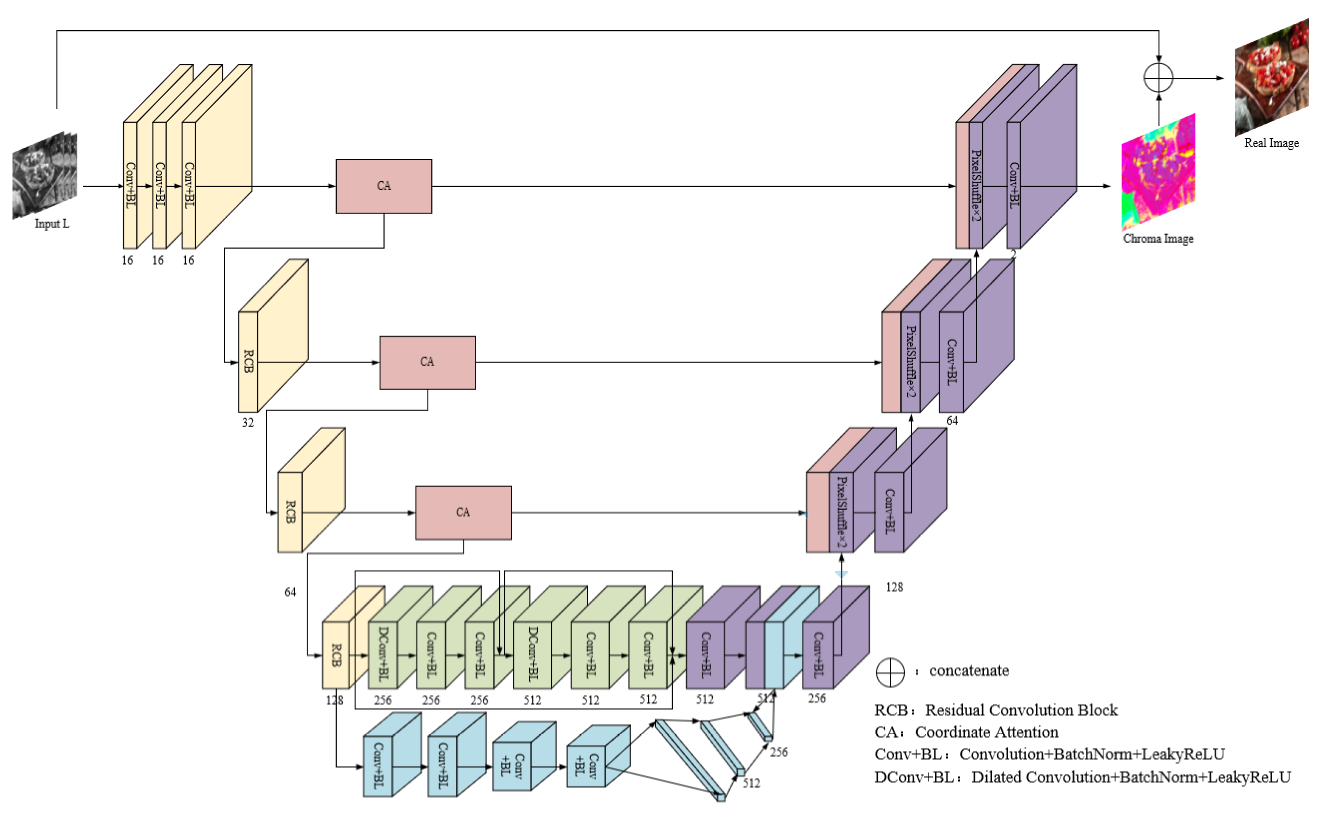
The generative network is designed based on the U-Net [19] network. The local feature-extraction subnet and the global feature-extraction subnet are used to achieve downsampling, and the coloring subnet is used to achieve upsampling. The local feature-extraction subnet is constructed by a residual structure, dilated convolution and attention mechanism and combined with the global feature-extraction subnet to fuse local features and global features, which can enhance the understanding of global semantic information. PixelShuffle [20] is introduced into the coloring subnet, and the local features of each scale obtained in the upsampling and downsampling process are integrated by skip connections, so that the network can pay attention to the context information to reduce the loss of texture and color information in the image coloring process.

(2)

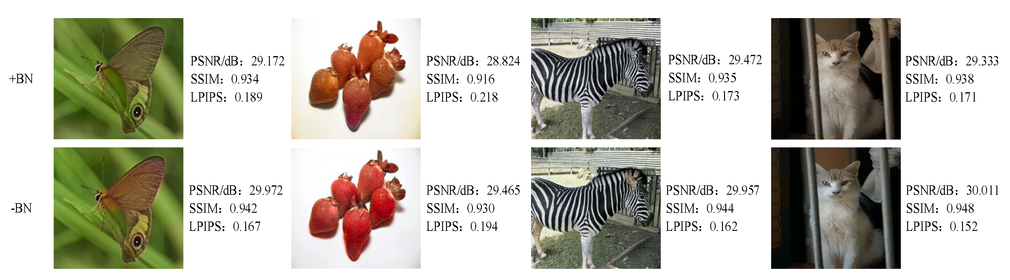
The batch normalization layer (BN) in the discriminative network is removed to reduce image artifacts and maintain image contrast.

(3)

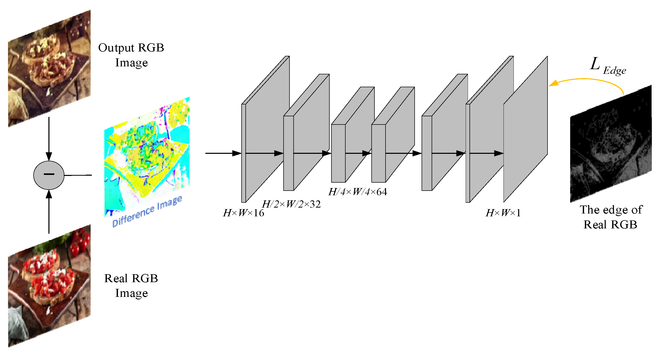
The edge-assisted network is designed, and the edge-assisted loss is introduced, and the loss function is optimized by combining it with the adversarial loss of relativistic average discriminator (RaGAN) [21], which can improve the constraint ability of the image color and edge and increase the robustness of the network.

Table 1. The comparison of the proposed method with some other image colorization methods.

Methods	Classification	Comparison
Levin et al. [7], Welsh et al. [8], etc.	Local-color-expansion-based methods	No need for huge image data. No automatic colorization, and manual assisted coloring is required; it takes a lot of time; the coloring effect of complex background images is poor, with inconsistent coloring, edge distortion and color crosstalk.
Xu et al. [9], Instance [10], Broad-GAN [11], etc.	Instance-based methods	It can be automatically colored to reduce time complexity; the coloring effect is significantly improved. The network structure is complex, and it is often only suitable for processing a certain type of image; the coloring effect depends on the quality of the provided instance image, which has great limitations.
Deoldify [15], ChromaGAN [16], Pix2PixGAN [18], CycleGAN [19], etc.	Deep-learning-based methods	The network structure is improved, which can realize the fast and automatic end-to-end coloring of various types of grayscale images, and the coloring authenticity is high. It needs the support of a huge image dataset; there are certain problems of color anomaly, border blooming and lack of contrast.
Proposed method	Deep-learning-based method	An end-to-end automatic colorization method for various types of grayscale images, including old photos; the network structure and the loss function are improved, and the ability for network semantic optimization and edge enhancement is enhanced, which can effectively colorize complex background images and alleviate the problems of abnormal color, blurred edges and lack of saturation. For some images with special complex background, the coloring effect needs to be improved.

Table 1. The comparison of the proposed method with some other image colorization methods.

Methods	Classification	Comparison
Levin et al. [7], Welsh et al. [8], etc.	Local-color-expansion-based methods	No need for huge image data. No automatic colorization, and manual assisted coloring is required; it takes a lot of time; the coloring effect of complex background images is poor, with inconsistent coloring, edge distortion and color crosstalk.
Xu et al. [9], Instance [10], Broad-GAN [11], etc.	Instance-based methods	It can be automatically colored to reduce time complexity; the coloring effect is significantly improved. The network structure is complex, and it is often only suitable for processing a certain type of image; the coloring effect depends on the quality of the provided instance image, which has great limitations.
Deoldify [15], ChromaGAN [16], Pix2PixGAN [18], CycleGAN [19], etc.	Deep-learning-based methods	The network structure is improved, which can realize the fast and automatic end-to-end coloring of various types of grayscale images, and the coloring authenticity is high. It needs the support of a huge image dataset; there are certain problems of color anomaly, border blooming and lack of contrast.
Proposed method	Deep-learning-based method	An end-to-end automatic colorization method for various types of grayscale images, including old photos; the network structure and the loss function are improved, and the ability for network semantic optimization and edge enhancement is enhanced, which can effectively colorize complex background images and alleviate the problems of abnormal color, blurred edges and lack of saturation. For some images with special complex background, the coloring effect needs to be improved.

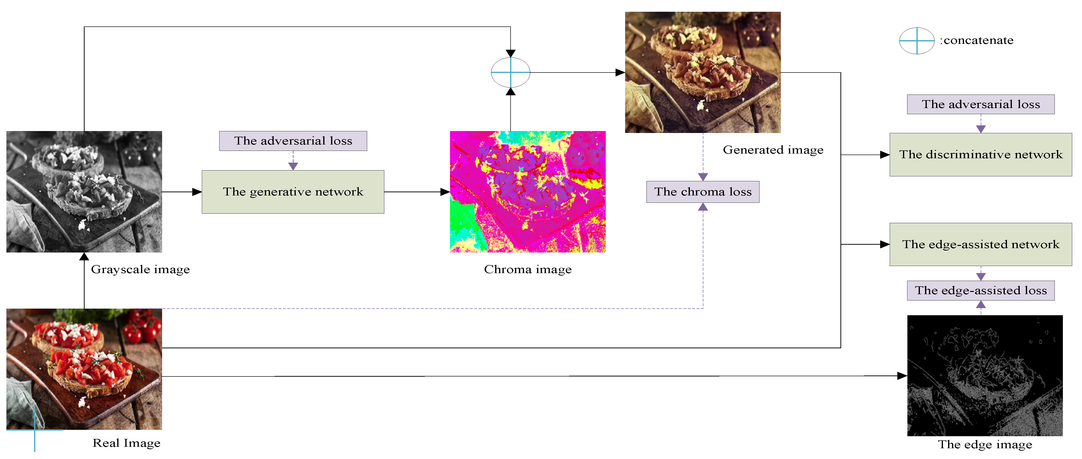
2. Proposed Method

Figure 1 is the flowchart of our method, which is described in detail as follows: Since the CIELab color space is based on the uniformity of human visual perception, its L luminance component can be regarded as the input grayscale image, and most features of the image are retained. Therefore, this paper is based on the CIELab color space to carry out work, and the size of input images are transformed into 224 × 224. Before the image is input to the network, it needs to be converted from the RGB color space to the Lab color space, and the L channel of the original image is used as the input of the network. The chroma image, which is output by the generative network, is concatenated with the input gray image to obtain the generated image. Then, the generated image and the real RGB image are input to the edge-assisted network and the discriminative network, so that the network parameters can be optimized by loss functions until the generative network and the discriminative network reach a game equilibrium state.

2.1. The Generative Network

The generative network is improved based on the U-Net network and its structure is shown in Figure 2. It mainly includes three subnets: the local feature-extraction subnet (G1, orange, green and red parts), the global feature-extraction subnet (G2, blue parts) and the coloring subnet (G3, red and purple parts). Firstly, local features and global features are extracted by stepwise downsampling with G1 and G2 and then fused. Finally, the RGB image is predicted by upsampling with G3.

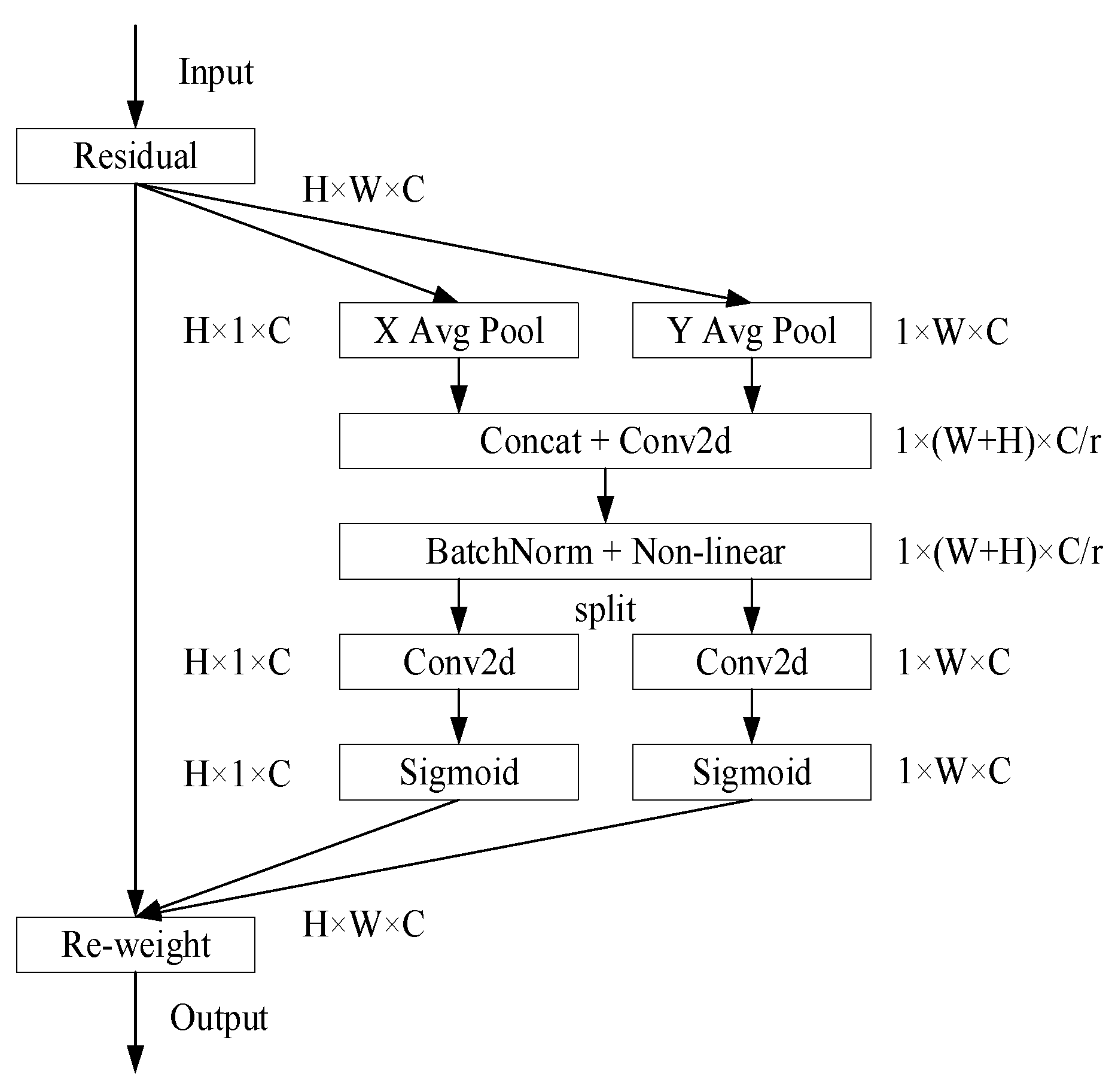
2.1.1. The Local Feature-Extraction Subnet

G1 can be divided into three parts: the shallow feature extraction, the downsampling and the deep feature extraction. More shallow features such as image edges are initially captured by using three 3 × 3 convolutions.

The downsampling consists of three residual convolution blocks (RCB), and the stride of the first convolutional layer in each RCB is 2, which is used for three downsampling operations. The structure of RCB is shown in Figure 3. The residual structure is used to robustly obtain the high-frequency information of the image, and simultaneously fuse contextual multi-scale features information to enhance the expression of semantic features and improve the loss of details in the feature-extraction process.

In order to obtain useful feature information more effectively, a novel coordinate attention (CA) module [22] is introduced before each RCB to reduce the influence of redundant features. On the one hand, CA can not only obtain cross-channel information but also capture direction and position information, so that appropriate features and key information can be extracted by the network. On the other hand, the CA module is very lightweight and can be flexibly used in various network frameworks. The more complex the background of an image is, the more difficult it is to extract its features. Feature integration through the CA module can make the network fully understand the foreground and background information of complex areas in images and effectively better semantic confusion. The CA module is shown in Figure 4.

Firstly, the input feature map is divided into two directions of width and height for global average pooling, respectively, in order to obtain the feature maps in these two directions. The process can be expressed by Formulas (1) and (2) [22]:

$$z_c^h\left(h\right)=\frac{1}{W}{\displaystyle \sum _{0\le i<W}{x}_c}\left(i,j\right)$$

(1)

$$z_c^w\left(w\right)=\frac{1}{H}{\displaystyle \sum _{0\le j<H}{x}_c}\left(j,w\right)$$

(2)

where $Z_c^h\left(h\right)$ and $Z_c^w\left(w\right)$ represent the component of the c-th channel at height h and at width w, respectively, and $x_c\left(h,i\right)$ and $x_c\left(j,w\right)$ represent the components of the input feature map of the c-th channel at coordinates $\left(h,i\right)$ and $\left(j,w\right)$.

Then, after concatenating the feature maps that obtain the global receptive field in two directions, the channel dimension is reduced to $C/r$ by a shared 1 × 1 convolutional function $F_1$, where $r$ is the reduction factor. Then, through the BN and the ReLU activation function, the intermediate feature maps encoding the spatial information in the width and height directions are obtained, as shown in Formula (3) [22]:

$$m=\epsilon \left(F_1\left(\lfloor z^h,z^w\rfloor \right)\right)$$

(3)

After that, $m$ is split into two separate tensors $m^h$ and $m^w$ according to the original height and width. The attention weight values $g^h$ and $g^w$ of $m^h$ and $m^w$ are obtained through two 1 × 1 convolution transformations $F_h$ and $F_w$ and the Sigmoid function $\sigma$. The process can be expressed by Formulas (4) and (5) [22]:

$$g^h=\sigma \left(F_h\left(m^h\right)\right)$$

(4)

$$g^w=\sigma \left(F_w\left(m^w\right)\right)$$

(5)

Finally, the output of the CA module can be written as Formula (6) [22]:

$$y_c\left(i,j\right)=x_c\left(i,j\right)\times g_c^h\left(i\right)\times g_c^w\left(j\right)$$

(6)

In this formula, $x_c\left(i,j\right)$ represents the input feature map, and $g_c^h\left(i\right)$ and $g_c^w\left(j\right)$ represent the attention weight values in the directions of the height and width, respectively.

Using convolution for downsampling all of the time will lead to the loss of more local information of images, but there are many deep features in the 28 × 28 feature maps that need to be further extracted, so two dilated convolutions (DConv) are used to replace the traditional downsampling operation, which aims to increase the receptive field of the network while maintaining the image resolution, reduce information loss and further extract deep information such as image semantic features. Considering the gridding effect caused by the dilated convolution, two 3 × 3 convolutions are added after each dilated convolution, and skip connections are added at the same time, so that the gridding phenomenon can be eliminated through the network’s self-learning.

2.1.2. The Global Feature-Extraction Subnet

Adding G2 after the third RCB, four convolutions in the form of Conv + BN + LeakyReLU (Conv + BL) are utilized by the subnet to achieve two downsampling and then through three fully connected layers to extract global features. Global features reflect the overall properties of the image, such as color, texture and structure, while local features reflect more detailed changes within image regions, such as detail information. The extracted global features are replicated and fused with the local features extracted by the last layer of G1, so that the network can effectively obtain rich feature information and fully focus on the global semantic information (such as scene layout and type, etc.), which can alleviate semantic confusion and avoid coloring errors. Let the size of the local feature map $f_l$ be $H\times W\times C_l$, the size of the global feature map $f_g$ be $1\times 1\times C_g$, and the fusion formula is shown in Formula (7):

$$f_{out}=\delta \left(b+\theta \left[{}_{C_p{\left(f_g\right)}_{H\times W}}^{f_l}\right]\right)$$

(7)

In this formula, $f_{out}$ is the output feature map, and its size is $H\times W\times C_l$. $\delta$ is the activation function; $C_p{\left(•\right)}_{H\times W}$ represents $H\times W$ times of replication, and $\theta$ and $b$ are the weight matrix and vector parameters that the network can learn.

2.1.3. The Coloring Subnet

G3 is used to generate color images, which mainly consists of two parts: upsampling and skip connections fused with CA modules. Upsampling is responsible for reconstructing the size, color and texture of images. There are various upsampling methods. Traditional methods such as deconvolution and uppooling tend to generate high computational complexity and introduce more additional information that are not conducive to image reconstruction [23]. In contrast, PixelShuffle is a more effective upsampling method. It not only has a higher computing speed but also can effectively improve the checkerboard effect existing in traditional upsampling methods. The main function of PixelShuffle is to combine the feature maps of $u^2$-times channels into the size of $W\times u$ and $H\times u$, as shown in Formula (8) [20]:

$$\left(N,u^{2}C,H,W\right)\to \left(N,C,H\times u,W\times u\right)$$

(8)

In this formula, $N$ represents the batch size, $u$ represents the upsampling ratio, $C$ represents the number of feature channels, and $H$ and $W$ represent the height and width of the feature map, respectively.

Three PixelShuffle operations of $u=2$ are used to generate an 8-times magnified image. Meanwhile, the low-dimensional feature information enhanced by the CA module in the downsampling is multiplexed into the high-dimensional feature information generated by the upsampling by skip connections at each scale, so as to make the high-dimensional features with rich semantic information and the low-dimensional features with detailed information complement each other to enhance the reconstruction effect of the upsampling.

2.2. The Edge-Assisted Network

Although the quality of generated images can be improved by global semantic optimization, there are still some problems. In the coloring process, the edge of images will become less clear, so that the predicted color image may have problems such as edge distortion, border color crosstalk and border sharpness degradation. In order to maintain a clear edge, an edge-assisted network is designed [24] to enhance the edge. The edge-assisted network is shown in Figure 5, and its structure is simple, with only two layers of downsampling and two layers of upsampling, which are realized by convolution with stride 2 and deconvolution. In this paper, this network is regarded as a loss network, and an edge-assisted loss function is designed to enhance the edge of the output RGB image and stabilize the textureless area. It is trained together with the generative network to jointly improve the network performance.

The input of the loss network is the difference image between the generated image and the original RGB image, and the output is the edge of the predicted RGB image. Most of the values in the edge image are equal to 0, which means that the loss network tries to make the value of the difference image tend to be 0 except the edge. So in order to make this network work better, the edge image of the original RGB image is taken as the sample image of the loss network to train, which not only achieves the effect of enhancing the edge, but also stabilizes the color area to a certain extent.

2.3. The Discriminative Network

If the discriminative network is too complex, it will be too powerful, which is not conducive to training the generative network. In the discriminative network, repeated convolutional layers and LeakyReLU activation functions are set up firstly to extract features, and then two fully connected layers are used to output the true and false probability through the Sigmoid function. After the image passes through the BN layer, its color distribution will be normalized, which will destroy the original contrast information and result in unpredictable artifacts. Therefore, the BN layer is removed in the discriminative network to suppress image artifacts, improve the color saturation and reduce the amount of network computation. The discriminative network parameters are shown in

Table 2. Discriminant network parameters.

Layer	Output Size	Layer	Output Size
s1-3 × 3-LeakyReLU	224 × 224	s1-3 × 3-LeakyReLU	56 × 56
s2-3 × 3-LeakyReLU	112 × 112	s2-3 × 3-LeakyReLU	28 × 28
s1-3 × 3-LeakyReLU	112 × 112	s1-3 × 3-LeakyReLU	1 × 1
s2-3 × 3-LeakyReLU	56 × 56	s1-3 × 3-LeakyReLU	1 × 1

.

2.4. The Design of Objective Loss Function

The standard discriminator of the GAN network is used to estimate the probability that the image input to the discriminator is a real image, which is prone to mode collapse and gradient disappearance during training, and the network is not easy to converge. While RaGAN tries to estimate the probability that the real image is more realistic than the generated image, its training is more stable, and the time to achieve optimal performance is greatly reduced [25]. RaGAN is denoted as $D_{\mathrm{Ra}}$, as shown in Formula (9) [25]:

$$D_{\mathrm{Ra}}\left(X_{\mathrm{R}},X_{\mathrm{F}}\right)=\sigma \left(C\left(X_{\mathrm{R}}\right)-E_{X_{\mathrm{F}}}\left[C\left(X_{\mathrm{F}}\right)\right]\right)$$

(9)

In this formula, $X_{\mathrm{R}}$ is the original RGB image, $X_{\mathrm{F}}$ is the generated image where $X_{\mathrm{F}}=G\left(X_{\mathrm{input}}\right)$, $X_{\mathrm{input}}$ is the input grayscale image, $E_{X_{\mathrm{F}}}\left[•\right]$ represents the operation of averaging all fake data in the mini-batch processing, and $C\left(•\right)$ represents the output of the nonlinear discriminator.

The $L_1$ norm is used to learn the two chroma values for each pixel and compute the chroma loss $L_{\mathrm{Color}}$, as shown in Formula (10):

$$L_{\mathrm{Color}}=E_{X_{\mathrm{input}}}{‖G\left(X_{\mathrm{input}}\right)-X_{\mathrm{R}}‖}_1$$

(10)

$L_{\mathrm{Color}}$ is a content loss that evaluates the distance between the generated image and the real image to avoid the colorization results being too flat and jumpy and to narrow the color error range.

The edge-assisted loss function $L_{\mathrm{Edge}}$ in the edge-assisted network is defined using the $L_2$ norm, as shown in Formula (11) [24]:

$$L_{\mathrm{Edge}}=E_{X_{\mathrm{R}}\_X_{\mathrm{F}}}{‖X_{\mathrm{F}\_\mathrm{Edge}}-X_{\mathrm{R}\_\mathrm{Edge}}‖}_2$$

(11)

In this formula, $X_{\mathrm{R}}\_X_{\mathrm{F}}$ is the input difference image, $X_{\mathrm{F}\_\mathrm{Edge}}$ is the edge image of the predicted image, and $X_{\mathrm{R}\_\mathrm{Edge}}$ is the edge image of the real image. $L_{\mathrm{Edge}}$ represents the pixel-level loss between the edge images of the difference image and the real image, mainly preserving the edge sharpness of the generated image.

The generative network loss includes chroma loss, adversarial loss and edge-assisted loss, as shown in Formula (12):

$$L_{\mathrm{G}}=-E_{X_{\mathrm{R}}}\left[\log \left(1-D_{\mathrm{Ra}}\left(X_{\mathrm{R}},X_{\mathrm{F}}\right)\right)\right]-E_{X_{\mathrm{F}}}\left[\log \left(D_{\mathrm{Ra}}\left(X_{\mathrm{F}},X_{\mathrm{R}}\right)\right)\right]+L_{\mathrm{Color}}+L_{\mathrm{Edge}}$$

(12)

The discriminative network loss function is shown in Formula (13):

$$L_D=-E_{X_{\mathrm{R}}}\left[\log \left(D_{\mathrm{Ra}}\left(X_{\mathrm{R}},X_{\mathrm{F}}\right)\right)\right]-E_{X_{\mathrm{F}}}\left[\log \left(1-D_{\mathrm{Ra}}\left(X_{\mathrm{F}},X_{\mathrm{R}}\right)\right)\right]$$

(13)

It can be seen that both the generative network and the discriminative network loss function benefit from the gradient of $X_{\mathrm{R}}$ and $X_{\mathrm{F}}$ in the adversarial training, so that the sharper edges and finer textures can be learned, and the naturalness and authenticity of the generated image can be improved.

3. Experiments and Analysis

3.1. Experimental Environment and Settings

• Dataset. In this paper, the network model is trained and tested based on the Places365 [26] and ImageNet [27] datasets. More than 1.8 million images of 365 different scenes are included in the Places365 [26] dataset. After filtering out a small number of grayscale images and dim images in the dataset, 15,000 images of different scenes are selected as the test set, and the remaining 1.68 million images are the training set. The ImageNet [27] dataset is a special database of the ILSVRC Challenge. In this paper, a subset of ImageNet [27] dataset is adopted. More than 1.2 million images of more than 1000 image categories are included in the ImageNet [27] dataset, and 10,000 images of different categories are selected as the test set, and the rest of the images are the training set. All images are pre-cropped to 224 × 224.
• Experimental Environment. The experiment is based on the Windows 10, and the deep learning framework Pytorch1.9.0 based on the CUDA-accelerated is used to build the network model. The hardwares are Intel Core i9 9900 K CPU with 64 GB of memory and NVIDIA GeForce RTX 3090 GPU with 24 GB of video memory.
• Training Settings. The discriminator is updated once per training, and the generator is updated twice per training. The optimizer chooses Adam; the weight decay is 0.005; the learning rate is set to 0.0003; the batch size is set to 32, and the iteration is 200 epochs.

3.2. Evaluation Indicators

The qualitative analysis and quantitative analysis are used to evaluate the quality of color images. The qualitative analysis is conducted according to the visual effect of the image, and the quantitative analysis adopts the peak signal-to-noise ratio (PSNR) [14], structural similarity (SSIM) [28] and learned perceptual image patch similarity (LPIPS) [29] as evaluation indicators. PSNR directly reflects the pixel-level mean square error between the generated image and the original image. The larger the value, the smaller the image distortion and the more reasonable the color distribution. SSIM is based on brightness, contrast and structure to measure images’ similarity. It reflects the subjective quality of images. The higher the value, the higher the degree of image restoration and the better the visual effect. LPIPS is a measure of learning-based perceptual similarity. Compared with PSNR and SSIM, LPIPS is more consistent with humans' perceptual judgment. The smaller the value, the smaller the perceptual difference between the generated image and the original image.

3.3. Comparison of Results of Different Methods

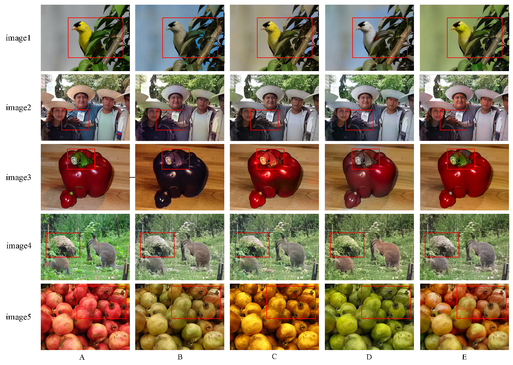
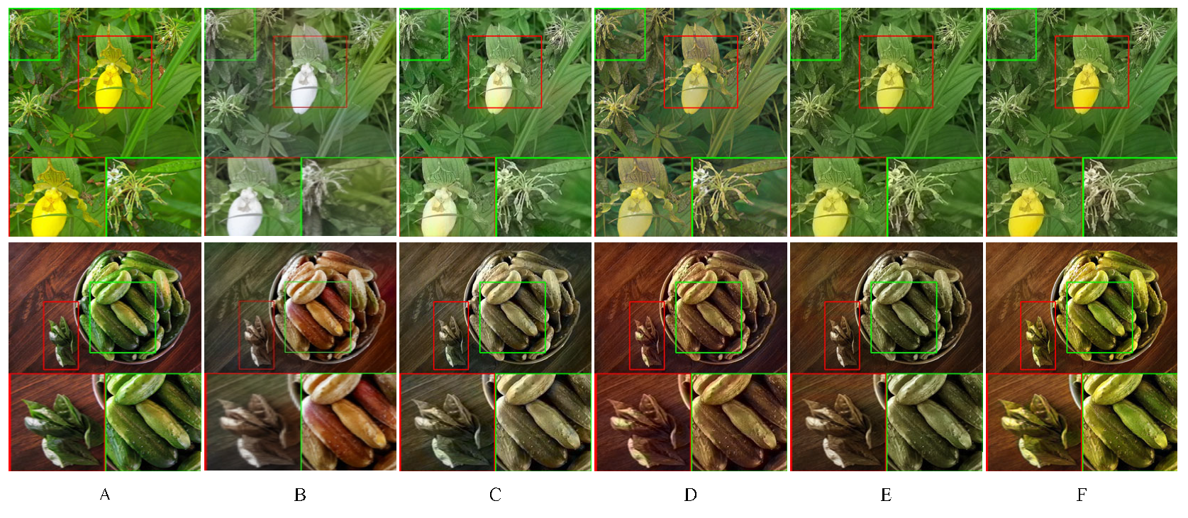
3.3.1. Comparison of Coloring Effects under the Original Image

In order to illustrate the effectiveness of the proposed method, it is compared with the existing excellent colorization methods (Reference [13], Deoldify [14] and ChromaGAN [15]). The experimental results are shown in Figure 6. The coloring effect of the comparison method adopts the final coloring model on its public website.

In Figure 6, the coloring effect of Ref. [13] is not good. The birds on the branches and the vegetables on the table are not colored reasonably, and the overall tone is single and the color is flat. Deoldify and ChromaGAN have better overall coloring effects. But the color in Deoldify is too aggressive and lacks a certain contrast, and the color smudge is obvious. ChromaGAN has higher visual comfort, but abnormal colors and color smudge are also serious, such as wrong colors of stones in front of animals and pomegranates, color smudge of girls’ clothes on boys’ hands and a lack of color saturation in the vegetables on the table.

In contrast, the proposed method not only has a better overall visual effect of the image but also has a good grasp of the coloring of the subtleties. In image 1, the boundary between birds and leaves is correctly distinguished, and more accurate coloring of birds and leaves is achieved. In image 2 and image 4, the smudge of girls’ clothes on boys’ hands and grass on stones are well-suppressed, and the coloring is more vivid and the contrast is higher. In image 3 and image 5, this method accurately identifies vegetables on the table and piled pomegranates and colors them in a reasonable color. It shows that the proposed method can enhance the understanding of the global semantic information and the processing effect of details; improve the ability to distinguish fuzzy boundaries; and effectively alleviate the problems of color anomaly, color overflow and lack of color saturation.

In order to objectively prove the effectiveness of the proposed method, three evaluation indicators selected in Section 3.2 are used to quantitatively evaluate the above coloring methods. The evaluation results are shown in

Table 3. Quantitative evaluation of the coloring results.

Method	Places365			ImageNet
	PSNR/dB	SSIM	LPIPS	PSNR/dB	SSIM	LPIPS
Ref. [13] Deoldify ChromaGAN	24.247 27.932 28.897	0.927 0.943 0.945	0.312 0.186 0.172	24.126 27.856 28.702	0.931 0.940 0.942	0.324 0.180 0.174
Proposed method	30.903	0.956	0.147	30.545	0.946	0.150

. As can be seen from Table 3, the PSNR, SSIM and LPIPS of the proposed method are 6.538 dB, 0.022 and 0.170 higher than Ref. [13] on average; 2.830 dB, 0.010 and 0.035 higher than Deoldify; and 1.925 dB, 0.008 and 0.025 higher than ChromaGAN, respectively, which is consistent with the qualitative analysis and reflects the superiority of the proposed method.

3.3.2. Comparison of the Coloring Effects of Old Black and White Photos

In order to further verify the superiority of our method, some old photos are selected to compare the coloring effects. The results are shown in Figure 7. It can be seen that our method compared with other three methods resulted in fewer abnormal colors and less boundary color leakage. The colors are more vivid, and the contrast is higher, which further proves the superiority of our method.

3.3.3. Comparison of Time Complexity

In order to test the performance of this model from multiple perspectives, 10,000 pairs of 224 × 224 pixel images are selected from the training set for 200 rounds of training, and 1000 grayscale images are selected from the test set for colorization. As can be seen from

Table 4. Time complexity test.

Model	Ref. [13]	Deoldify	ChromaGAN	Proposed Method
Average training time/s	0.22	0.34	0.43	0.25
Average coloring time/s	0.14	0.26	0.33	0.18

, the average training time of this model is 0.25 s, and the average coloring time is 0.18 s, which is lower time complexity for training and testing than other methods.

3.4. Ablation Experiments

In order to better verify the effectiveness of each module, three ablation experiments are set up for training separately. Ablation experiments are conducted in the same experimental environment as the above-mentioned comparison experiment.

3.4.1. The Ablation Experiments 1

In order to clarify the effectiveness of the network structure in this paper, by fixing the proposed method’s loss function, five different structures are designed for ablation experiments: (1) U-Net: The generative network adopts the original U-Net network, (2) U-Net + G1: G1 replaces the original U-Net downsampling part, (3) U-Net + G3: G3 replaces the original U-Net upsampling part, (4) G1 + G3, (5) G1 + G2 + G3: the proposed method. So the effects of the designed local feature-extraction subnet G1, global feature-extraction subnet G2 and coloring subnet G3 on the network performance can be respectively verified. The same local area in generated images of different methods is enlarged, and the results are shown in Figure 8.

It can be observed from Figure 8 that the image coloring effect of the original U-Net network is not good, that its edges are blurred, and that there are many abnormal colors. After G1 replacement, the restoration effect of image color, edge and contrast is significantly improved, and the effect of G3 replacement is slightly inferior to G1 replacement, which embodies the efficiency of G1 feature extraction. The image authenticity of G1 + G3 is further improved; not only the abnormal color is reduced, but also the color is more saturated and vivid. But there are also some features that are not fully extracted, such as the coloring error of green leafy vegetables next to cucumbers. However, the proposed method based on G1 + G3 adds the G2 subnet, which obviously improves the global and local color recovery effect of images, and its coloring quality is the best. It indicates that the design of the G1, G2 and G3 structures in this paper can improve the ability of network representation and strengthen the network's understanding of local feature information and global semantic information.

Table 5. Ablation experiment of the network structure.

Model	Places365			ImageNet
	PSNR/dB	SSIM	LPIPS	PSNR/dB	SSIM	LPIPS
U-Net U-Net + G1 U-Net + G3 G1 + G3	23.462 26.484 25.672 29.133	0.919 0.934 0.923 0.945	0.323 0.204 0.272 0.165	23.032 26.368 25.804 28.821	0.921 0.930 0.925 0.938	0.344 0.193 0.266 0.172
Proposed method	30.903	0.956	0.147	30.545	0.946	0.150

shows the results of ablation experiment 1. It can be seen from Table 5 that, compared with the original U-Net structure, the indicators of the other four structures have been improved. The indicator of our method is the highest, which reflects the superior semantic optimization ability of the network structure of our method.

3.4.2. The Ablation Experiments 2

In order to clarify the influence of removing the BN layer in the discriminative network on the network performance, two different structures are designed for ablation experiments: (1) +BN: There is the BN layer in the discriminative network, (2) −BN: The proposed method. The results are shown in Figure 9. As can be seen from the Figure 9, the overall coloring effect of the two structures is relatively close, but −BN has better visual perception, higher color constraint and less boundary blooming, indicating that removing the BN layer of the discriminant network in this paper can improve the network coloring effect.

3.4.3. The Ablation Experiments 3

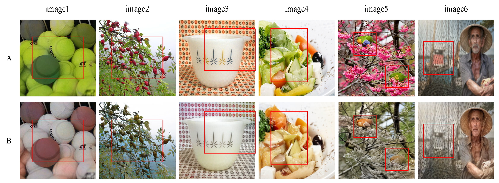
In order to clarify the effectiveness of the loss function in this paper, by fixing the proposed method’s generative network, three different structures are designed for ablation experiments: (1) GAN: The loss function is $L_{\mathrm{Color}}$ and the standard GAN loss, (2) RaGAN: The loss function is $L_{\mathrm{Color}}$ and RaGAN loss, (3) $L_{\mathrm{Edge}}$ + RaGAN: The proposed method, so the effects of the RaGAN loss and edge-assisted loss can be respectively verified. The local magnification of the colored image is performed, and the result is shown in Figure 10. Compared with the standard GAN loss, the RaGAN loss has greatly improved the contrast and edge clarity, but the ladybugs are not correctly colored, while our method has high contrast, clear edges and reasonable coloring of the ladybugs, indicating that the $L_{\mathrm{Edge}}$ loss can effectively preserve the image edges, stabilize the color regions and improve the image quality.

3.5. Failure Cases

We show six examples of failure cases in Figure 11. In image 1–4, a large number of objects overlap and repeat, which results in a great difference between the coloring image and the original image. However, since image colorization is a multi-modal problem, image 1 and image 3 still have certain reliability. In image 5–6, birds are covered with flowers and the boat is occluded by the fishing net. It is difficult for our network to accurately identify these occluded objects, resulting in incorrect coloring. In these cases, the coloring methods of Ref. [13], Deoldify [14] and ChromaGAN [15] are more different from the original image, and the color of the image is single, and the problems of semantic confusion, color crosstalk and edge blurring are more serious. For example, birds that are severely occluded by branches are not recognized, and the visual effect lacks authenticity. Therefore, although the coloring ability of our method needs to be improved for images with a great number of overlapping and repeated objects and blurred details caused by occlusion, it has already improved the coloring effect of images with complex backgrounds.

3.6. Discussions

This paper mainly studies the grayscale image colorization algorithm based on deep learning. Considering that the coloring results of the existing algorithms are generally correct, there are still some problems. For example, the network structure is too complex, which leads to a relatively large time cost; the designed algorithm is not portable and can only achieve accurate coloring of a certain type of image; the coloring lacks saturation, and it is easy to cause coloring errors due to semantic confusion, and there are some phenomena such as color crosstalk and insufficient color richness.

To improve these problems, an adversarial image colorization method based on semantic optimization and edge enhancement is proposed. Our work is to re-improve the network structure and design the loss function so that the model can fully understand semantic information and enhance edges to reduce abnormal colors and suppress border blooming, while enriching image colors. The datasets Places365 [25] and ImageNet [26] cover most real-life scenarios. In Section 3.3 and Section 3.4, we have verified that our method achieves excellent results on the datasets, and the method also shows superior performance on old photo colorization. At the same time, we have also verified that our method has a lower time complexity.

But the datasets are preprocessed before network training to remove some dim images, because too many dim images are not good for network training and colorization. Therefore, the quality of the images in the datasets affects the performance of our algorithm.

In Section 3.5, the failure cases are analyzed. Our method is not satisfactory for images with a large number of overlapping or repeated objects and blurred details caused by a large number of occlusions. Therefore, the network structure, loss function and training strategy of this paper need to be further studied to be suitable for image coloring in more complex scenes.

4. Conclusions

An adversarial image colorization method based on semantic optimization and edge preservation is proposed in this paper. The local feature-extraction subnet and the global feature-extraction subnet are used to fuse the features of different scales and layers, so as to effectively utilize the information of different feature layers, fully understand the global semantic information and effectively recognize fuzzy boundaries and suppress detail loss by combining PixelShuffle and the attention mechanism. The loss function in this paper combines the chroma loss and edge-assisted loss on the basis of RaGAN, which can not only color the edges more accurately but also restore richer and brighter colors. The experimental results show that, compared with the other three methods, the proposed method has a certain improvement in PSNR, SSIM and LPIPS on the two types’ datasets, more reasonable color distribution in perception and higher authenticity, which proves that the proposed method can effectively alleviate the problems of semantic blur, boundary overflow and lack of color saturation in the process of image colorization.

In the next stage of research, the design of our method will be improved for image coloring problems in complex scenes such as fuzzy details, object occlusion and a large number of repeated objects to further enhance the generalization of our method.

References

1. Zhao, Y.Z.; Po, L.M.; Cheung, K.W.; Yu, W.Y.; Rehman, Y.A.U. SCGAN: Saliency Map-Guided Colorization with Generative Adversarial Network. IEEE Trans. Circuits Syst. Video Technol. 2021, 31, 3062–3077. [Google Scholar] [CrossRef]
2. Wu, Y.Z.; Wang, X.T.; Li, Y.; Zhang, H.L.; Zhao, X.; Shan, Y. Towards vivid and diverse image colorization with generative color prior. In Proceeding of the 2021 IEEE/CVF International Conference on Computer Vision, Montreal, QC, Canada, 10–17 October 2021; pp. 14357–14366. [Google Scholar]
3. Zhuo, L.; Tan, S.; Li, B.; Huang, J.W. ISP-GAN: Inception Sub-Pixel Deconvolution-Based Lightweight GANs for Colorization. Multimed. Tools Appl. 2022, 81, 24977–24994. [Google Scholar] [CrossRef]
4. Morra, L.; Piano, L.; Lamberti, F.; Tommasi, T. Bridging the gap between natural and medical images through deep colorization. In Proceeding of the 2021 IEEE International Conference on Pattern Recognition, Milan, Italy, 10–15 January 2021; pp. 835–842. [Google Scholar]
5. Liu, S.; Gao, M.L.; John, V.J.; Liu, Z.; Blasch, E. Deep Learning Thermal Image Translation for Night Vision Perception. ACM Trans. Intell. Syst. Technol. 2021, 9, 1–18. [Google Scholar] [CrossRef]
6. Wan, Z.Y.; Zhang, B.; Chen, D.D.; Zhang, P.; Chen, D.; Liao, J. Bringing old photos back to life. In Proceedings of the 2020 IEEE Conference on Computer Vision and Pattern Recognition, Seattle, WA, USA, 13–19 June 2020; pp. 2744–2754. [Google Scholar]
7. Levin, A.; Lischinski, D.; Weiss, Y. Colorization Using Optimization. ACM Trans. Graph. 2004, 23, 689–694. [Google Scholar] [CrossRef]
8. Welsh, T.; Ashikhmin, M.; Mueller, K. Transferring Color to Greyscale Images. ACM Trans. Graph. 2002, 21, 277–280. [Google Scholar] [CrossRef]
9. Xu, Z.Y.; Wang, T.T.; Fang, F.M.; Sheng, Y.; Zhang, G.X. Stylization-based architecture for fast deep exemplar colorization. In Proceedings of the 2020 IEEE Conference on Computer Vision and Pattern Recognition, Seattle, WA, USA, 13–19 June 2020; pp. 9360–9369. [Google Scholar]
10. Su, J.W.; Chu, H.K.; Huang, J.B. Instance-aware image colorization. In Proceedings of the 2020 IEEE Conference on Computer Vision and Pattern Recognition, Seattle, WA, USA, 13–19 June 2020; pp. 7965–7974. [Google Scholar]
11. Li, H.X.; Sheng, B.; Li, P.; Ali, R.; Chen, C.L.P. Globally and Locally Semantic Colorization via Exemplar-Based Broad-GAN. IEEE Trans. Image Process. 2021, 30, 8526–8539. [Google Scholar] [CrossRef] [PubMed]
12. Zhang, R.; Isola, P.; Efros, A.A. Colorful image colorization. In Proceedings of the European Conference on Computer Vision, Amsterdam, The Netherlands, 11–14 October 2016; pp. 649–666. [Google Scholar]
13. Zhang, R.; Zhu, J.Y.; Isola, P. Real-Time User-Guided Image Colorization with Learned Deep Priors. ACM Trans. Graph. 2017, 36, 1–11. [Google Scholar] [CrossRef]
14. Jason, A. Colorizing and Restoring Photos and Video. Available online: https://github.com/jantic/DeOldify (accessed on 16 January 2022).
15. Vitoria, P.; Cisa, L.R.; Ballester, C. Chroma GAN: Adversarial picture colorization with semantic class distribution. In Proceedings of the 2020 IEEE Winter Conference on Applications of Computer Vision, Snowmass, CO, USA, 1–5 March 2020; pp. 2434–2443. [Google Scholar]
16. Radford, A.; Metz, L.; Chintala, S. Unsupervised representation learning with deep convolutional generative adversarial network. arXiv 2015, arXiv:1511.06434. [Google Scholar]
17. Isola, P.; Zhu, J.Y.; Zhou, T.H.; Efros, A.A. Image-to-image translation with conditional adversarial networks. In Proceedings of the 2017 IEEE Conference on Computer Vision and Pattern Recognition, Honolulu, HI, USA, 21–26 July 2017; pp. 5967–5976. [Google Scholar]
18. Zhu, J.Y.; Park, T.; Isola, P.; Efros, A.A. Unpaired image-to-image translation using cycle-consistent adversarial networks. In Proceedings of the 2017 IEEE International Conference on Computer Vision, Venice, Italy, 22–29 October 2017; pp. 2242–2251. [Google Scholar]
19. Ronneberger, O.; Fischer, P.; Brox, T. U-Net: Convolutional networks for biomedical image segmentation. In Proceedings of the International Conference on Medical Image Computing and Computer-Assisted Intervention, Munich, Germany, 5–9 October 2015; pp. 234–241. [Google Scholar]
20. Shi, W.Z.; Caballero, J.; Huszár, F.; Totz, J.; Aitken, A.P.; Bishop, R. Real-time single image and video super-resolution using an efficient sub-pixel convolutional neural network. In Proceedings of the 2016 IEEE Conference on Computer Vision and Pattern Recognition, Las Vegas, NV, USA, 27–30 June 2016; pp. 1874–1883. [Google Scholar]
21. Jolicoeur-Martineau, A. The relativistic discriminator: A key element missing from standard GAN. arXiv 2018, arXiv:1807.00734v3. [Google Scholar]
22. Hou, Q.B.; Zhou, D.Q.; Feng, J.S. Coordinate attention for efficient mobile network design. In Proceedings of the 2021 IEEE Conference on Computer Vision and Pattern Recognition, Nashville, TN, USA, 20–25 June 2021; pp. 13708–13717. [Google Scholar]
23. Jiang, Y.C.; Liu, Y.Q.; Zhan, W.D.; Zhu, D.P. Light Weight Dual-Stream Residual Network for Single Image Super-Resolution. IEEE Access 2021, 9, 129890–129901. [Google Scholar] [CrossRef]
24. Dong, Z.; Kamata, S.I.; Breckon, T.P. Infrared image colorization using a s-shape network. In Proceedings of the IEEE International Conference on Image Processing, Athens, Greece, 7–10 October 2018; pp. 2242–2246. [Google Scholar]
25. Wang, X.T.; Yu, K.; Wu, S.X.; Gu, J.J.; Liu, Y.H.; Dong, C. ESRGAN: Enhanced super-resolution generative adversarial networks. In Proceedings of the European Conference on Computer Vision, Munich, Germany, 8–14 September 2018; pp. 63–79. [Google Scholar]
26. Zhou, B.; Lapedriza, A.; Khosla, A.; Oliva, A.; Torralba, A. Places: A 10 Million Image Database for Scene Recognition. IEEE Trans. Pattern Anal. Mach. Intell. 2018, 40, 1452–1464. [Google Scholar] [CrossRef] [PubMed]
27. Deng, J.; Dong, W.; Socher, R.; Li, J.; Li, K.; Li, F.F. ImageNet: A large-scale hierarchical image database. In Proceedings of the 2009 IEEE Conference on Computer Vision and Pattern Recognition, Miami, FL, USA, 20–25 June 2009; pp. 248–255. [Google Scholar]
28. Zhu, D.P.; Zhan, W.D.; Jiang, Y.C.; Xu, X.Y.; Guo, R.Z. MIFFuse: A Multi-Level Feature Fusion Network for Infrared and Visible Images. IEEE Access 2021, 9, 130778–130792. [Google Scholar] [CrossRef]
29. Zhang, R.; Isola, P.; Efros, A.A.; Shechtman, E.; Wang, O. The unreasonable effectiveness of deep features as a perceptual metric. In Proceedings of the 2018 IEEE Conference on Computer Vision and Pattern Recognition, Salt Lake City, UT, USA, 18–23 June 2018; pp. 586–595. [Google Scholar]
Figure 1. The flowchart of our method.
Electronics 11 03006 g001
Figure 2. The structure of generator.
Electronics 11 03006 g002
Figure 3. The structure of the residual convolution block.
Electronics 11 03006 g003
Figure 4. The coordinate attention module.
Electronics 11 03006 g004
Figure 5. The edge-assisted network structure.
Electronics 11 03006 g005
Figure 6. Comparison of the coloring effects of different colorization methods. (A) Real image; (B) Ref. [13]; (C) Deoldify; (D) ChromaGAN; (E) proposed method. The red rectangular box represents the area where the colorization effect of each method differs greatly.
Electronics 11 03006 g006
Figure 7. Comparison of the coloring effects of black and white old photos. (A) Grayscale image; (B) Ref. [13]; (C) Deoldify; (D) ChromaGAN; (E) Proposed method. The red rectangular box represents the area where the colorization effect of each method differs greatly.
Electronics 11 03006 g007
Figure 8. The results of the ablation experiment 1. (A) Real image; (B) U-Net; (C) U-Net + G1; (D) U-Net + G3; (E) G1 + G3; (F) Proposed method. The red and green rectangular box represent the area where the colorization effect of each method differs greatly and enlarged images of the area.
Electronics 11 03006 g008
Figure 9. The results of the ablation experiment 2.
Electronics 11 03006 g009
Figure 10. The results of the ablation experiment 3. (A) Real image; (B) GAN; (C) RaGAN; (D) Proposed method. The red rectangular box represents the area where the colorization effect of each method differs greatly and the enlarged image of the area.
Electronics 11 03006 g010
Figure 11. Failure cases. (A) Real image; (B) Proposed method. The red rectangular box represents the area where the colorization effect of each method differs greatly.
Electronics 11 03006 g011