Article

A Content-Aware Non-Local Means Method for Image Denoising

Institute of Robotics and Intelligent Systems, School of Information Science and Engineering, Wuhan University of Science and Technology, Wuhan 430081, China
*
Author to whom correspondence should be addressed.
Electronics 2022, 11(18), 2898; https://doi.org/10.3390/electronics11182898
Submission received: 22 July 2022 / Revised: 9 September 2022 / Accepted: 9 September 2022 / Published: 13 September 2022

Abstract

:
Parameter setting and information redundancy are essential issues for the non-local means (NLM) algorithm. This paper introduces a new factor based on the Hessian matrix to adapt the smoothing parameter. Then, a strategy is proposed to implement the NLM by representing patches in terms of features, which uses the 2D histogram and summed-area table. Compared with other methods, the metric for patch similarity in this paper is based on statistical features of patches instead of Euclidean distance. More importantly, not many predefined thresholds are needed. Experimental results show that the proposed algorithm obtains better visual quality and numerical results, especially for images with rich contents and high noise.

1. Introduction

Denoising is one of the fundamental problems in image processing. Non-local mean (NLM) [1] is one of the most representative denoising algorithms based on patch, which utilizes the redundancy and similarity among the various parts of the image [2].
Considering a noise image I R M × N , let I ( v ) and I 0 ( v ) be the noisy and noise-free image pixels at position v, respectively. The noisy image can be mathematically modeled as [1]:
I ( v ) = I 0 ( v ) + γ ( v )
where γ ( y ) is a Gaussian additive white noise with zero mean and standard deviation (SD) σ > 0 . The output of the NLM method [1] is computed as follows:
I ^ ( u ) = v Ω W ( u , v ) I ( v ) / v Ω W ( u , v )
where I ^ ( u ) represents the denoised intensity at pixel u in the image domain Ω , and W ( u , v ) denotes a weight depending on the similarity between patches centered at positions u and v, satisfying W ( u , v ) 0 .
Let P ( u ) and P ( v ) denote the square neighborhood of size B × B and centered at pixels u and v, respectively. Then the similarity W ( u , v ) of the intensity gray level vectors P ( u ) and P ( v ) can measure two pixels u and v. W ( u , v ) is determined by the pixel Gaussian-weighted Euclidean distance P ( u ) P ( v ) 2 [1]:
W ( u , v ) = 1 Z ( u ) e x p ( P ( u ) P ( v ) 2 h 2 )
where Z ( u ) = v e x p ( P ( u ) P ( v ) 2 h 2 ) is the normalization factor, and h is the smoothing parameter controlling the filtering degree.
It is seen from Equations (1) and (2) that the critical idea of NLM is to find similar patches. It is worth noting that the computational complexity is O ( B 2 M 2 N 2 ) [1], which is too expensive to be used in practical applications.
To reduce computation, Buades et al. [3] proposed to search similar patches in a relatively large “search window” of size S × S instead of the whole image, which modifies the initial NLM method into a semi-local means solution. The computational complexity is then reduced to O ( S 2 B 2 M N ) . After that, various NLM speed-up approaches were introduced, which can be classified into three categories: (1) fast operators, for example, using FFT [4], convolution [5]; (2) data-driven lower dimensional subspace of image neighborhoods, such as using SVD [6], PCA [7], optimization learning [8,9]; (3) preselection methods, i.e., eliminating dissimilar pixels in computation. The typical criteria for preclassification include mean and gradient [10], mean and SD [11,12], moments [13], or cluster tree [14].
Another issue associated with the NLM method is the choice of the filtering parameter h, which controls the smoothing of image details. In [1], Buades suggested that the parameter is proportional to the noise SD σ . Zeng et al. [15] used structure tensors according to region properties to adjust the smoothing parameter, which is sensitive to high noise levels. Verma et al. [16] proposed a gray relational analysis-based adaptive smoothing parameter in every pixel, assuming the signal is smooth. Panigrahi et al. [17] considered that many delicate structures and small details are as oscillatory as noise; thus, they introduced three curvelet scales to denoise both the smooth and oscillatory noise. Nevertheless, as mentioned by the authors, this method cannot preserve the details at low noise strength.
It is well known that the long-standing challenge in image denoising comes from the fact that while noise is removed, the image edges and details are preserved. The denoising strength should differ among image regions, namely, smooth, edge, and texture. Motivated by the above two issues, a fast content-aware NLM method is proposed in this paper. Specifically, this work introduces an adaptive smoothing parameter based on the Hessian matrix to solve the problem of different noise levels, which can adjust smoothing according to image content. A new patch preclassification is derived such that each patch is represented by its statistical features without repetitive computation. The use of a 2D histogram provides a fast global search of similar patches. Experimental results show that the proposed algorithm obtains good visual quality and numerical results, especially for images with rich contents and high noise.
In the following section, the effect of the NLM smoothing parameter h is tested and analyzed in Section 2, which presents an adaptive filtering parameter based on the Hessian matrix in Section 3. A new patch preclassification is derived in Section 4. The fast search of similar patches from a 2D histogram is described in Section 5. The experimental results are demonstrated in Section 6, and the conclusions follow.

2. Effect of Image Content on NLM Smoothing Parameter

In NLM, the smoothing parameter h is selected as
h = k σ
where k is a constant. In this section, the effect of image contents on the smoothing parameter is tested, as shown in Figure 1.
Figure 2 shows the PSNRs in different smoothing parameters controlled by parameter k. It is observed that (1) an optimal smoothing parameter exists for each image; (2) the optimal smoothing parameter is content-dependent, i.e., the smoothing parameter for complex contents such as (c) and (e) is less than that for simple contents such as (b) or (g); (3) the optimal smoothing parameter is independent of noise strength. These observations reveal that the smoothing parameter should be content-adaptive, and an adaptive strategy based on Hessian matrix analysis is proposed in the following section.

3. Content-Aware Smoothing Parameter Selection via Hessian Matrix Analysis

The pixel variation mainly expresses the local content of the image. Hessian matrix H ( p ) exactly describes second-order intensity variations surrounding a chosen pixel region p = ( x , y ) [18]. Assuming that f ( x , y ) is a function of p, then the Hessian matrix of p is mathematically defined as:
H ( p ) = H x x H x y H y x H y y = 2 f x 2 2 f x y 2 f y x 2 f y 2
where 2 f x 2 , 2 f x y , 2 f y x , and 2 f y 2 are second-order partial derivatives of the region. The image second-order derivatives can be taken by convolving the image with derivatives of Gaussian G ( x , y ; Π ) = 1 2 π Π 2 e x 2 + y 2 2 Π 2 using the Gaussian scale-space techniques, where Π is a scale factor [19]. The Hessian matrix H ( p ) is a positive definite that has two eigenvalues.
The eigenvalues of H ( p ) at the pixel ( x , y ) are as follows:
λ 1 = 1 2 ( H x x + H y y + ( H x x H y y ) 2 + 4 H x y 2 ) λ 2 = 1 2 ( H x x + H y y ( H x x H y y ) 2 + 4 H x y 2 )
The relationship between the eigenvalues reveals image content (edge, smooth, and texture regions [17]) [18]. For example, the difference of eigenvalues on edge regions is significant, i.e., λ 1 λ 2 . The two eigenvalues from the corners, texture regions, or smooth regions are approximately the same, i.e., λ 1 λ 2 , and the eigenvalues are large on corners or texture regions and small on smooth regions.
Theoretically, the filtering parameter should be more prominent on smooth regions and smaller on texture regions. For distinguishing edges from the smooth region, a ratio r is introduced below:
r = | λ 1 | | λ 2 |
Thus, a new term k ^ , which can measure content, is proposed as follows:
k ^ = 0.7 r ( 1 e F / t )
where 0.7 is a recommendation factor from [1], t = 0.3 δ is an experimental parameter, δ is the SD of local content, and F is defined as:
F = | λ 1 | + | λ 2 |
which reveals intensity information. The restraint F can distinguish corners and smooth regions.
The Canny operator is introduced to extract edges simultaneously to implement the content-aware NLM for well achieving edge-preserving. Then, the proposed new adaptive filtering parameter h ^ aiming at the edge and non-edge regions is selected in the following way:
e d : h ^ = k ^ α σ e d : h ^ = k ^ β σ
where α and β are empirical values, e d denotes edge regions, and e d is non-edge regions (smooth and texture regions) [20]. In edge regions, r is far smaller than 1 when the exponent of k ^ is α , and the filtering parameter h ^ is small enough to preserve edges. Regarding non-edge regions, r is close to 1. Then, the exponent of k ^ is β , which leads h ^ to be more significant to denoise.

4. Representing Euclidean Distance of Patches in Terms of Statistical Features

The key idea of the NLM method is to use Euclidean distance to measure the similarity of patches; however, searching similar patches and calculating Euclidean distance is time-consuming. In the following, we represent the Euclidean distance of patches in terms of statistical features such that the distance computation is efficient.
For a given patch P u , the Euclidean distance between P u and an arbitrary patch P x can be expressed as follows:
d ( P u , P x ) = P u P x 2 = E { [ P u P x ] 2 } = E { ( P u ) 2 2 P u P x + ( P x ) 2 } = E ( ( P u ) 2 ) + E ( ( P x ) 2 ) 2 E ( P u P x ) = ( D ( P u ) + ( E ( P u ) ) 2 ) + ( D ( P x ) + ( E ( P x ) ) 2 ) 2 E ( P u P x )
where E ( P u ) , D ( P u ) are the mean and variance of P u , respectively.
In Equation (11), E ( P u ) , D ( P u ) , E ( P x ) , and D ( P x ) can be precalculated independently, but the term E ( P u P x ) cannot. Fortunately, the following Lemma provides an efficient method to compute this term.
Lemma 1.
Assuming two Gaussian distributions, whose means and standard deviations are μ 1 and μ 2 , σ 1 and σ 2 , respectively, the product of the two Gaussian distributions is approximate to a Gaussian distribution:
τ = 1 2 π ( σ 1 2 + σ 2 2 ) e x p [ ( μ 1 μ 2 ) 2 2 ( σ 1 2 + σ 2 2 ) ] .
with mean and SD as follows:
μ 12 = μ 1 σ 2 2 + μ 2 σ 1 2 σ 1 2 + σ 2 2 a n d σ 12 = σ 1 2 σ 2 2 σ 1 2 + σ 2 2
The proof of the Lemma is demonstrated in Appendix A.
Therefore, the Euclidean distance between two patches P u and P x can be independently computed as follows:
d ( P u , P x ) = P u P x 2 = D ( P u ) + ( E ( P u ) ) 2 + D ( P x ) + ( E ( P x ) ) 2 2 E ( P u ) D ( P x ) + E ( P x ) D ( P u ) D ( P x ) + D ( P u )
By this way, the following statistical relationship exists:
D ( P u ) = [ S ( P u ) ] 2
where S ( P u ) is the standard deviation (std) of P u . In addition, we ignore the comparison of noise-free patches and the similarity between a noise-free and a noisy version of a patch because the noise distribution of different regions is hard to estimate [21].
Equation (12) reveals that the Euclidean distance between two patches can be represented by the underlying patch features, i.e., mean and std. It is evident that mean and std can independently be computed and stored. Thus, the issue of finding similar patches becomes a search strategy in terms of the statistical features. A 2D histogram of statistical features is described to search for similar patches quickly.

5. The Search Strategy of Similar Patches from 2D Histogram

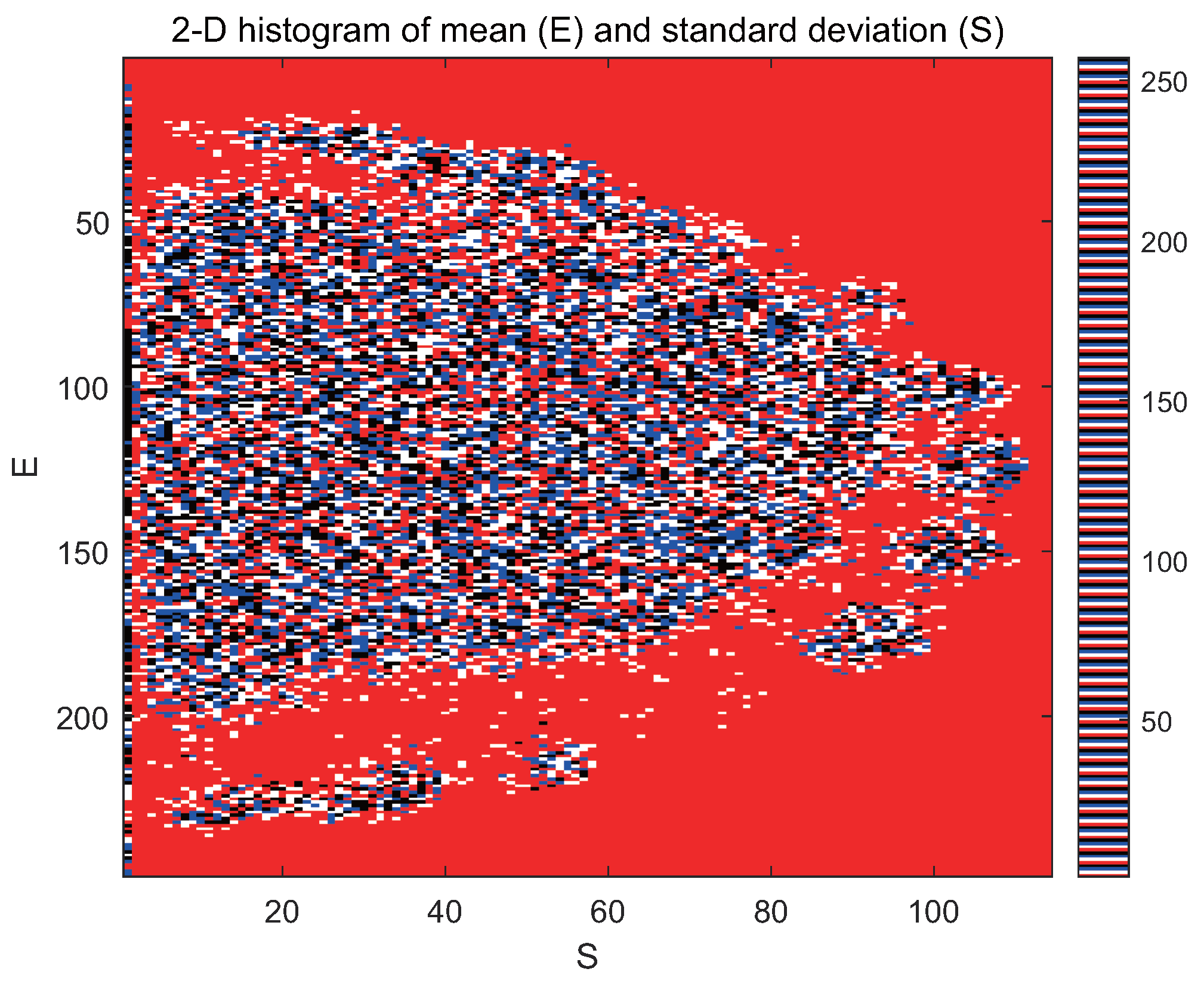
5.1. 2D Histogram to Represent Statistical Features

For a noisy image, I R M × N , E ( P u ) , S ( P u ) R M × N for each patch P u R B × B are obtained. Let N e , N s be total bins in E ( u ) and S ( u ) , respectively, and the variables E ( u ) and S ( u ) can be correlated by 2D histogram Φ ( E , S ) R N e × N s shown in Figure 3. For example, Φ ( E 1 , S 2 ) indicates the number which satisfies E ( i , j ) = E 1 and, S ( i , j ) = S 2 simultaneously. The 2D histogram directly reveals the distribution of patch features.

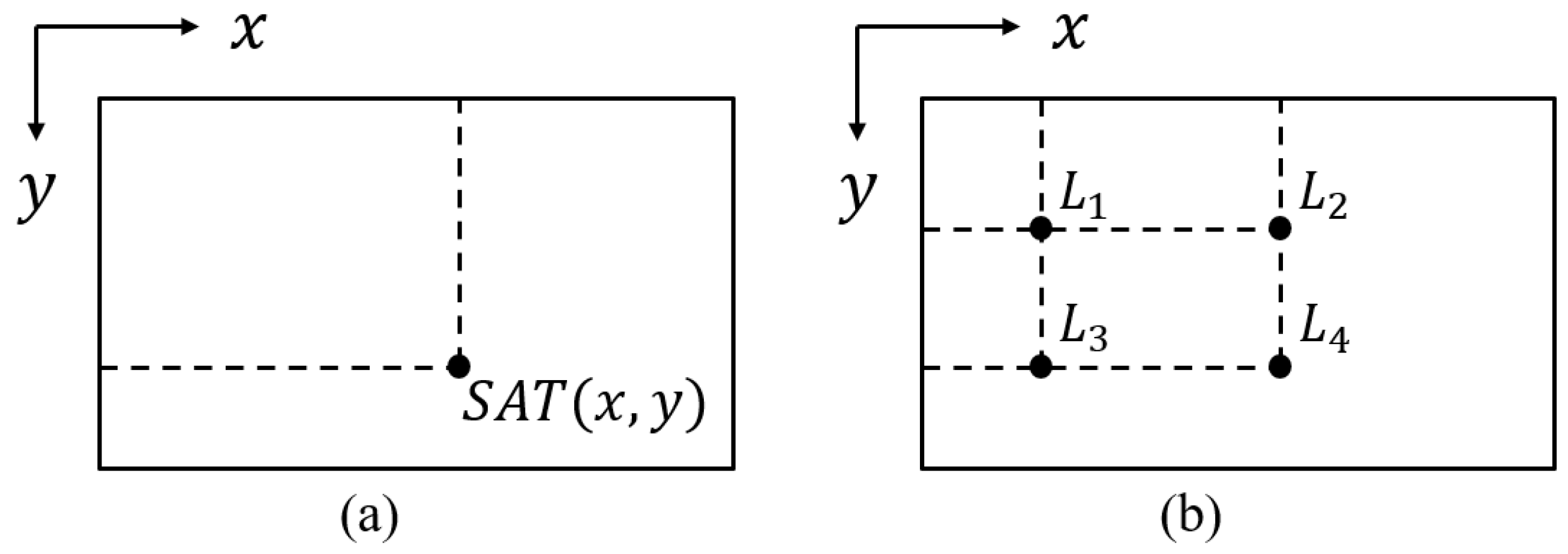
5.2. Summed-Area Table for Fast Searching Similar Patches

For a specific patch P i , the number of similar patches can be directly found from the 2D histogram. Iteratively searching for similar good patches in the whole feature domain is time-consuming if few similar patches are found. Thus, the summed-area table [22] is employed to improve search speed.
A summed-area table, denoted S A T ( x , y ) , represents the sum of values located in the upper left rectangular region of location Φ ( x , y ) , which is defined as follows [22]:
S A T ( x , y ) = x x , y y Φ ( x , y )
As shown in Figure 4, the sum of a rectangular region can be easily obtained by
L 1 ( x ) x L 4 ( x ) , L 1 ( y ) y L 4 ( y ) Φ ( x , y ) = L 4 + L 1 L 2 L 3
where L is the same as S A T ( x , y ) , and L can be obtained according to the 2D histogram shown in Figure 3. Then, Equation (15) calculates the number of similar patches and obtains their statistical features simultaneously. It is seen from Equation (15) that the search of similar patches by the summed-area table is only three addition and subtraction operations.

5.3. Threshold for Searching Patches

The degree of similarities between reference patch P i and arbitrary patch exists witha threshold η to balance whether the results act best. However, it is hard to select the best threshold to obtain the best PSNR or SSIM. Figure 5 indicates the tendency of PSNR with different thresholds when noise SD is 35. As the threshold increases, the PSNR rises fast and then tends to plateau. If η is too small, some helpful information will be lost. While η is larger, there are enough patches that contain similar information; though some dissimilar patches are recorded, their effect can be ignored most of the time. The results merely show slight fluctuation after searching enough patches.
As a result, the threshold is defined as follows:
η = ρ Ω
where ρ is a scale factor, and Ω is the color variance of the image.
The search for similar patches depends on selecting the threshold to a relatively great degree, which affects the denoising results.
In summary, the proposed method achieves a global search of similar patches instead of a semi-local means method. The computational complexity of the proposed method is O ( M N ) . The proposed algorithm consists of four parts:
(1)
Analyze the eigenvalues of each image pixel based on the Hessian matrix, then use the Canny operator to obtain an adaptive filtering parameter h ^ .
(2)
Represent Euclidean distance of patches in terms of statistical features.
(3)
Obtain a 2D histogram based on statistical features.
(4)
Search the similar patches according to a 2D histogram with a regular threshold based on summed area table.
(5)
Denoise the noisy image using a patchwise process such as NLM in the remaining steps.

6. Experimental Results

This section shows the experimental results on various real images with different types of noises. To evaluate the performance of the results of our method, we compared it with five state-of-the-art algorithms: NAMF [23], FastHD-NLM [24], SNN [25], CNLM [26], and LMM-RP [27]. Thirty typical images from the USC-SIPI Image Database [28] and Image Databases (https://www.imageprocessingplace.com/root_files_V3/image_databases.htm, accessed on 7 June 2022), shown in Figure 1, are chosen for the experiments. In addition, the patch size used for denoising is 7 × 7 ; α and β in (10) are 0.6 and 0.35, respectively; ρ in (16) is 10 in this work. All experiments are performed on AMD 1700X 3.40 GHz with 16 GB memory.
The remainder of this section is organized as follows. First, the image house with many smooth regions and the image cameraman with more textures are compared in case of different noise levels σ = { 5 , 10 , 20 , 30 , 40 , 50 } . Then we compare our algorithm with other algorithms. Finally, we explore the performance of our algorithm.

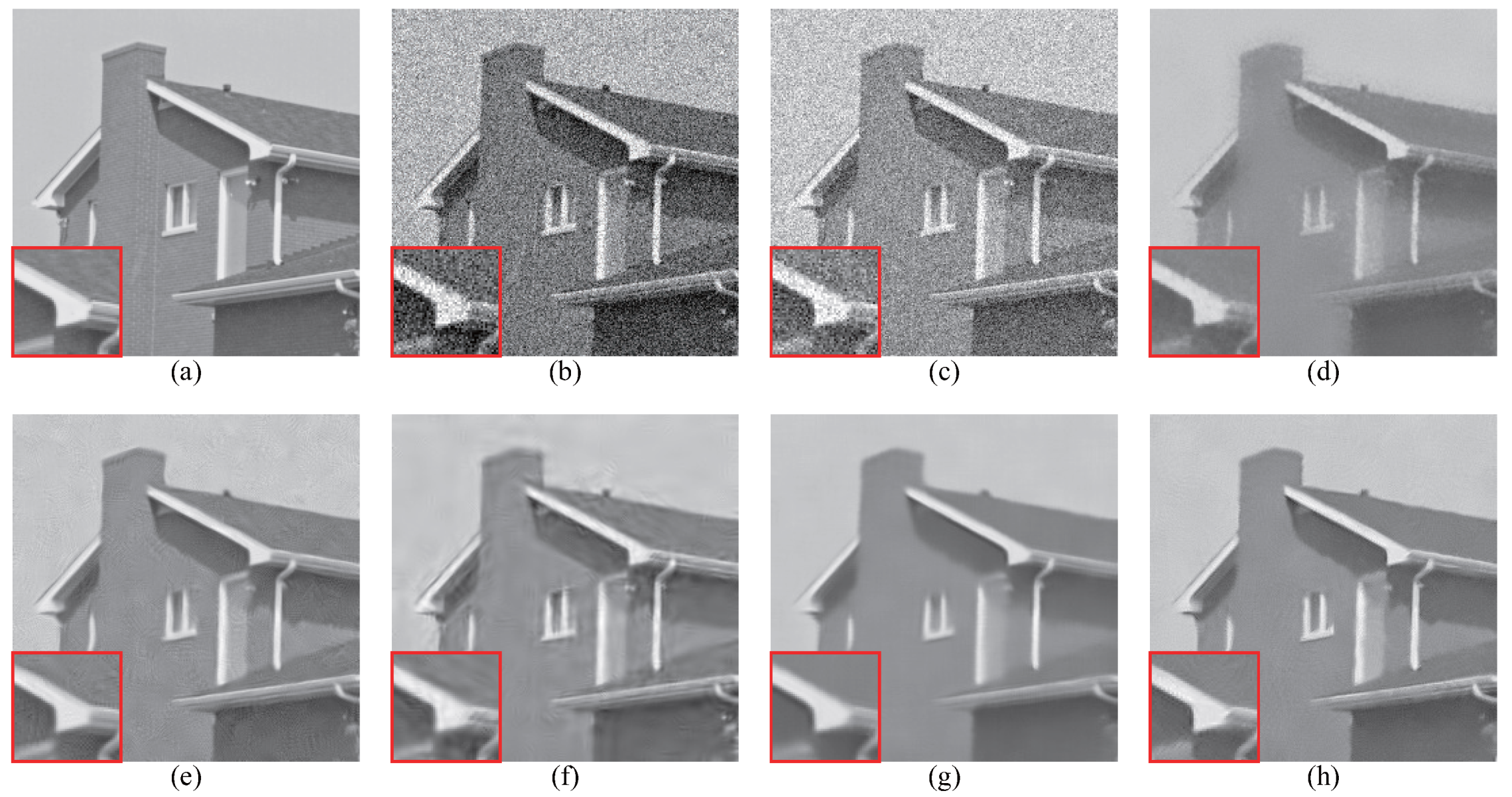
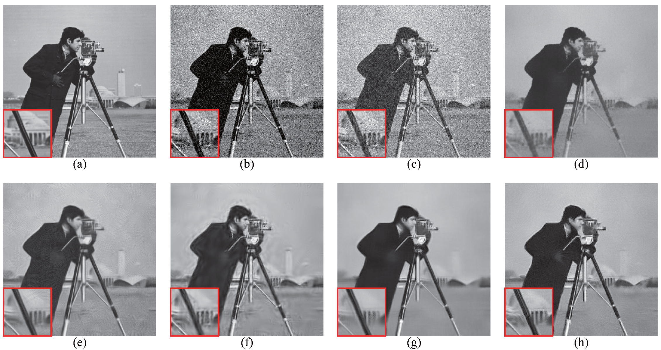
6.1. Image with Smooth Regions

The smooth regions of the image usually have similar intensities, whose denoising results in less fluctuation when tested in any algorithms, while the filtering window still influences their performances. Figure 6 compares denoised results on the house image with σ = 30 . FastHD-NLM, LMM-RP, and the proposed algorithm aim at the smooth regions and obtain better results. By observing the enlarged area in Figure 6, we can see that NAMF performs poorly. While FastHD-NLM, SNN, and CNLM still exist, much complicated information is caused by the Gaussian noise. Although LMM-RP denoises well, it blurs more edge at the same time. The proposed algorithm is better at the edge regions, which is more natural.
The curves of PSNR and SSIM with standard deviations σ = { 5 , 10 , 20 , 30 , 40 , 50 } are shown in Figure 7. Figure 7 indicates that the proposed algorithm obtains higher PSNR and SSIM simultaneously. With the increasing noise level, the performances of the proposed algorithm contain better effects.

6.2. Image with Complex Regions

It is harder to denoise the images with more complex textures, especially for the edge regions. This enlarged area shows the complicated regions of Figure 8 and can compare the denoised effects. SNN and LMM-RP blur too much to lose some details, while NAMF, FastHD-NLM, and CNLM still contain noise and even produce distortion. The proposed algorithms can denoise well and save better edge information than the above algorithms. As shown in Figure 8, the proposed algorithm is good at preserving the structural information and edge sharpness from the visible results.
Figure 9 shows the curves of PSNR and SSIM for the cameraman image. With the noise level increasing, the PSNR and SSIM of the proposed algorithm show superior performance, which indicates its robustness to a certain degree.

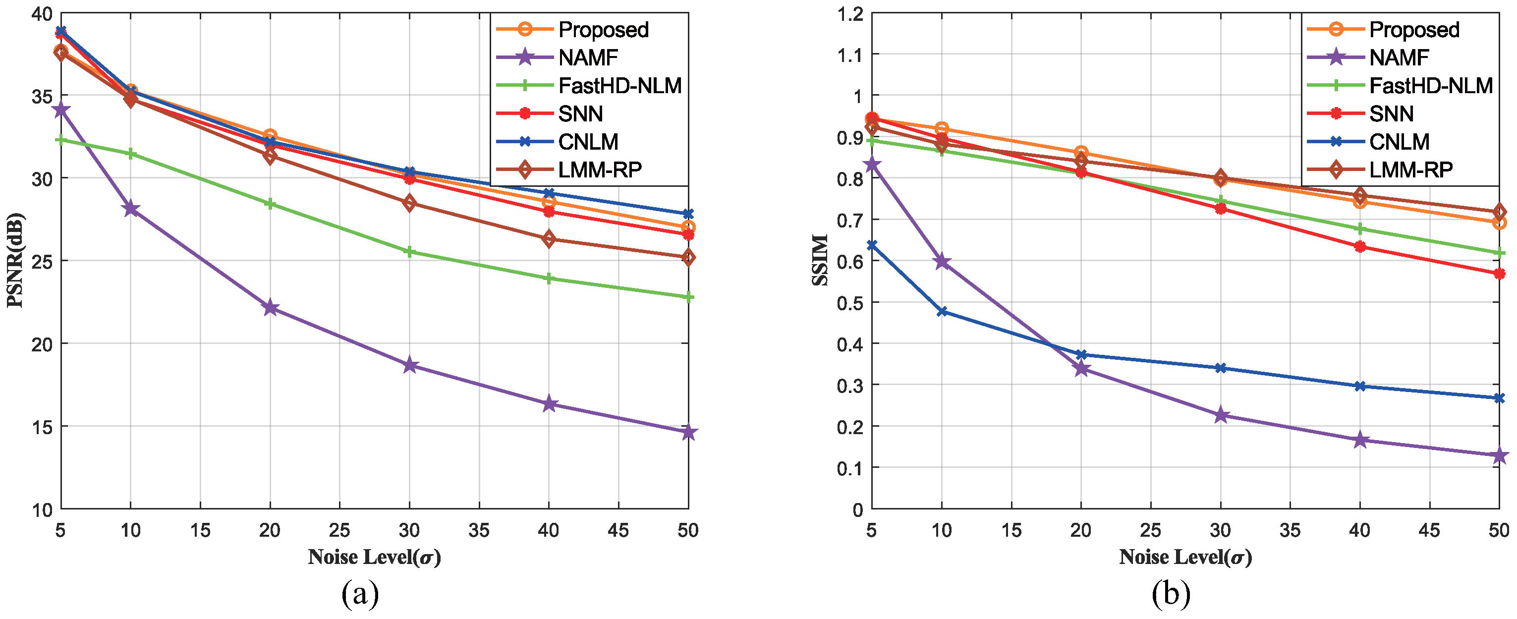
6.3. Synthetical Comparison

We select several typical images with smooth (Pepper, Plane, and Lake) or complex (Barbara, Lena, Flinstones, and Hill) regions and compare their PSNR and SSIM in Table 1 with different noise standard deviations (The bold numbers are best results.). For images with non-edge regions, the proposed algorithm performs better than the other ones. When noise std is low, the proposed algorithm obtains similar results; its superiority emerges after the image is corrupted more. Due to random noise SD, the values transform a little, but the proposed algorithm still performs stably. For the edge, the noise distribution limits the results when the noise std becomes larger.
We compare the average PSNR and SSIM on 30 images as well. It is observed from Table 2 that the proposed algorithm achieves better results. With the noise level increasing, the values of the proposed algorithm decrease more gently. From Table 2, we can see that our algorithm is more effective in texture and tiny details. Moreover, it performs well in the homogeneous areas of the image as well. Because the proposed algorithm adopts the global search strategy, it can find all the similar patches in the image rather than being limited to a search window. Therefore, the proposed algorithm can record global information to search for the most similar patch compared to other algorithms.
Finally, we compare the execution times of several algorithms spent on 30 images with all the standard deviations: FastHD-NLM: 436.698 s, SNN: 165.667 s, CNLM: 980.629 s, LMM-RP: 339.392 s, NAMF: 20.373 s, and ours: 253.64 s. Our algorithm did not take much longer time.
Combining the above analyses, we can see that the proposed algorithm obtains better visual effect and objective estimations, especially for the high noisy images or regions with rich contents. While the proposed algorithm adopts the patch search strategy, the texture will still be blurred to a certain extent, which is an unavoidable issue to be solved in future work.

7. Conclusions

A fixed-filter parameter and local search for similar patches greatly limit the denoising performance of the NLM-based method. Considering the parameter adaptation and search efficiency, a new filter parameter of the NLM method based on the Hessian matrix and Euclidean distance re-expression is proposed in this paper. Specifically, a content-aware parameter with different filtering degrees in different regions based on the derivatives of Hessian matrix eigenvalues is proposed first. In order to make full use of the global information of the image, the Euclidean distance is re-expressed as the std and mean of the patch, which is precalculated and stored to speed up the search for similar patches. In particular, a Euclidean distance threshold is designed to select similar patches when calculating the similarity of patches. Experimental results show that the proposed method has obvious denoising performance advantages for images with complex textures and high noise levels.

Author Contributions

Conceptualization, S.F.; methodology, S.F.; software, S.F.; validation, S.F. and J.W.; formal analysis, J.W. and S.W.; investigation, S.F.; resources, S.F. and S.W.; data curation, S.F.; writing—original draft preparation, S.F.; writing—review and editing, S.W.; visualization, S.F.; supervision, S.W.; project administration, S.W.; funding acquisition, S.W. All authors have read and agreed to the published version of the manuscript.

Funding

This research was funded by the National Natural Science Foundation of China under Grants 61775172, 61371190, and Hubei Key Technical Innovation Project under Grant ZDCX2019000025.

Institutional Review Board Statement

Not applicable.

Informed Consent Statement

Not applicable.

Data Availability Statement

Not applicable.

Acknowledgments

We thank Zhang, H., Nair, P., Frosio, I., Yamanappa, W., and Nguyen, M.P. for supporting the open-access publication of this paper.

Conflicts of Interest

The authors declare no conflict of interest.

Appendix A

Given two Gaussian PDFs:
P 1 ( x ) = 1 2 π σ 1 e ( x μ 1 ) 2 2 σ 1 2 a n d P 2 ( x ) = 1 2 π σ 2 e ( x μ 2 ) 2 2 σ 2 2
The product gives
P 1 ( x ) P 2 ( x ) = 1 2 π σ 1 σ 2 e ( ( x μ 1 ) 2 2 σ 1 2 + ( x μ 2 ) 2 2 σ 2 2 )
Define the term in the exponent
t = ( x μ 1 ) 2 2 σ 1 2 + ( x μ 2 ) 2 2 σ 2 2
Then expand two right terms in powers of x to give
t = ( σ 1 2 + σ 2 2 ) x 2 2 ( μ 1 σ 2 2 + μ 2 σ 1 2 ) x + μ 1 2 σ 2 2 + μ 2 2 σ 1 2 2 σ 1 2 σ 2 2
Dividing through by the coefficient of x 2 gives
t = x 2 2 ( μ 1 σ 2 2 + μ 2 σ 1 2 ) x σ 1 2 + σ 2 2 + μ 1 2 σ 2 2 + μ 2 2 σ 1 2 σ 1 2 + σ 2 2 2 σ 1 2 σ 2 2 σ 1 2 + σ 2 2
Adding this term in (A2) gives
P 1 ( x ) P 2 ( x ) 1 2 π σ 1 σ 2 e ( x 2 2 ( μ 1 σ 2 2 + μ 2 σ 1 2 ) x σ 1 2 + σ 2 2 + μ 1 2 σ 2 2 + μ 2 2 σ 1 2 σ 1 2 + σ 2 2 2 σ 1 2 σ 2 2 σ 1 2 + σ 2 2 )
According to the usual Gaussian form, the product of two Gaussian PDFs is proportional to a Gaussian PDF with the following mean and standard deviation, i.e.,
σ 12 = σ 1 2 σ 2 2 σ 1 2 + σ 2 2 a n d μ 12 = μ 1 σ 2 2 + μ 2 σ 1 2 σ 1 2 + σ 2 2
Then we can proceed from (A5) to obtain the scaling constant explicitly. Suppose that δ is the term required to complete the square in t, i.e.,
δ = ( μ 1 σ 2 2 + μ 2 σ 1 2 σ 1 2 + σ 2 2 ) 2 ( μ 1 2 σ 2 2 + μ 2 2 σ 1 2 σ 1 2 + σ 2 2 ) 2 2 σ 1 2 σ 2 2 σ 1 2 + σ 2 2 = 0
Adding this term to t gives
t = x 2 2 ( μ 1 σ 2 2 + μ 2 σ 1 2 ) x σ 1 2 + σ 2 2 + μ 1 2 σ 2 2 + μ 2 2 σ 1 2 σ 1 2 + σ 2 2 2 σ 1 2 σ 2 2 σ 1 2 + σ 2 2 + ( μ 1 σ 2 2 + μ 2 σ 1 2 σ 1 2 + σ 2 2 ) 2 ( μ 1 2 σ 2 2 + μ 2 2 σ 1 2 σ 1 2 + σ 2 2 ) 2 2 σ 1 2 σ 2 2 σ 1 2 + σ 2 2
Then t transforms to
t = ( x μ 1 σ 2 2 + μ 2 σ 1 2 σ 1 2 + σ 2 2 ) 2 2 σ 1 2 σ 2 2 σ 1 2 + σ 2 2 + ( μ 1 μ 2 ) 2 2 ( σ 1 2 + σ 2 2 ) = ( x μ 12 ) 2 2 σ 12 2 + ( μ 1 μ 2 ) 2 2 ( σ 1 2 + σ 2 2 )
Substituting back into (A2) gives
P 1 ( x ) P 2 ( x ) = 1 2 π σ 1 σ 2 e ( x μ 12 ) 2 2 σ 12 2 e ( μ 1 μ 2 ) 2 2 ( σ 1 2 + σ 2 2 ) = 1 2 π σ 12 e ( x μ 12 ) 2 2 σ 12 2 1 2 π σ 1 2 + σ 2 2 e ( μ 1 μ 2 ) 2 2 ( σ 1 2 + σ 2 2 )
Therefore, the product of two Gaussian PDFs P 1 ( x ) and P 2 ( x ) is a scaled Gaussian PDF
P 1 ( x ) P 2 ( x ) = S 2 π σ 12 e ( x μ 12 ) 2 2 σ 12 2
where τ is the scaling factor on both μ 1 and μ 2 with standard deviation σ 1 2 + σ 2 2
τ = 1 2 π σ 1 2 + σ 2 2 e ( μ 1 μ 2 ) 2 2 ( σ 1 2 + σ 2 2 )

References

  1. Buades, A.; Coll, B.; Morel, J. A non-local algorithm for image denoising. In Proceedings of the 2005 IEEE Computer Society Conference on Computer Vision and Pattern Recognition (CVPR’05), San Diego, CA, USA, 20–25 June 2005; pp. 60–65. [Google Scholar]
  2. Alkinani, M.H.; El-Sakka, M.R. Patch-based models and algorithms for image denoising: A comparative review between patch-based images denoising methods for additive noise reduction. EURASIP J. Image Video Process. 2017, 2017, 58. [Google Scholar] [CrossRef] [PubMed]
  3. Buades, A.; Coll, B.; Morel, J. A review of image denoising algorithms, with a new one. Multiscale Model. Simul. 2005, 4, 490–530. [Google Scholar] [CrossRef]
  4. Deledalle, C.; Duval, V.; Salmon, J. Non-local methods with shape-adaptive patches (NLM-SAP). J. Math. Imaging Vis. 2012, 43, 103–120. [Google Scholar] [CrossRef]
  5. Yin, R.; Gao, T.; Lu, Y.M.; Daubechies, I. A tale of two bases: Local-nonlocal regularization on image patches with convolution framelets. SIAM J. Imaging Sci. 2017, 10, 711–750. [Google Scholar] [CrossRef]
  6. Guo, Q.; Zhang, C.; Zhang, Y.; Liu, H. An efficient SVD-based method for image denoising. IEEE Trans. Circ. Syst. Video 2015, 26, 868–880. [Google Scholar] [CrossRef]
  7. Yousif, O.; Ban, Y. Improving urban change detection from multitemporal SAR images using PCA-NLM. IEEE Trans. Geosci. Remote Sens. 2013, 51, 2032–2041. [Google Scholar] [CrossRef]
  8. Cai, S.; Kang, Z.; Yang, M.; Xiong, X.; Peng, C.; Xiao, M. Image denoising via improved dictionary learning with global structure and local similarity preservations. Symmetry 2018, 10, 167. [Google Scholar] [CrossRef]
  9. Cai, S.; Liu, K.; Yang, M.; Tang, J.; Xiong, X.; Xiao, M. A new development of non-local image denoising using fixed-point iteration for non-convex p sparse optimization. PLoS ONE 2018, 13, e208503. [Google Scholar] [CrossRef]
  10. Mahmoudi, M.; Sapiro, G. Fast image and video denoising via nonlocal means of similar neighborhoods. IEEE Signal Proc. Lett. 2005, 12, 839–842. [Google Scholar] [CrossRef]
  11. Tristán-Vega, A.; García-Pérez, V.; Aja-Fernández, S.; Westin, C. Efficient and robust nonlocal means denoising of MR data based on salient features matching. Comput. Methods Programs Biol. 2012, 105, 131–144. [Google Scholar] [CrossRef] [Green Version]
  12. Duval, V.; Aujol, J.; Gousseau, Y. A bias-variance approach for the nonlocal means. SIAM J. Imaging Sci. 2011, 4, 760–788. [Google Scholar] [CrossRef]
  13. Dauwe, A.; Goossens, B.; Luong, H.Q.; Philips, W. A fast non-local image denoising algorithm. In Proceedings of the Image Processing: Algorithms and Systems VI, San Jose, CA, USA, 28–29 January 2008; pp. 324–331. [Google Scholar]
  14. Brox, T.; Kleinschmidt, O.; Cremers, D. Efficient nonlocal means for denoising of textural patterns. IEEE Trans. Image Process. 2008, 17, 1083–1092. [Google Scholar] [CrossRef]
  15. Zeng, W.; Du, Y.; Hu, C. Noise suppression by discontinuity indicator controlled non-local means method. Multimed. Tools Appl. 2017, 76, 13239–13253. [Google Scholar] [CrossRef]
  16. Verma, R.; Pandey, R. Grey relational analysis based adaptive smoothing parameter for non-local means image denoising. Multimed. Tools Appl. 2018, 77, 25919–25940. [Google Scholar] [CrossRef]
  17. Panigrahi, S.K.; Gupta, S.; Sahu, P.K. Curvelet-based multiscale denoising using non-local means & guided image filter. IET Image Process. 2018, 12, 909–918. [Google Scholar]
  18. Frangi, A.F.; Niessen, W.J.; Vincken, K.L.; Viergever, M.A. Multiscale vessel enhancement filtering. In Proceedings of the International Conference on Medical Image Computing and Computer-Assisted Intervention, Cambridge, MA, USA, 11–13 October 1998; pp. 130–137. [Google Scholar]
  19. Lindeberg, T. Scale-Space Theory in Computer Vision; Springer Science & Business Media: Berlin, Germany, 2013; Volume 256. [Google Scholar]
  20. Starck, J.; Elad, M.; Donoho, D.L. Image decomposition: Separation of texture from piecewise smooth content. In Wavelets: Applications in Signal and Image Processing X; SPIE: Bellingham, WA, USA, 2003; pp. 571–582. [Google Scholar]
  21. Deledalle, C.; Denis, L.; Tupin, F. How to compare noisy patches? Patch similarity beyond Gaussian noise. Int. J. Comput. Vis. 2012, 99, 86–102. [Google Scholar] [CrossRef]
  22. Crow, F.C. Summed-area tables for texture mapping. In Proceedings of the 11th Annual Conference on Computer Graphics and Interactive Techniques, Minneapolis, MN, USA, 23–27 July 1984; pp. 207–212. [Google Scholar]
  23. Zhang, H.; Zhu, Y.; Zheng, H. NAMF: A nonlocal adaptive mean filter for removal of salt-and-pepper noise. Math. Probl. Eng. 2021, 2021, 4127679. [Google Scholar] [CrossRef]
  24. Nair, P.; Chaudhury, K.N. Fast high-dimensional bilateral and nonlocal means filtering. IEEE Trans. Image Process. 2018, 28, 1470–1481. [Google Scholar] [CrossRef]
  25. Frosio, I.; Kautz, J. Statistical nearest neighbors for image denoising. IEEE Trans. Image Process. 2018, 28, 723–738. [Google Scholar] [CrossRef]
  26. Yamanappa, W.; Sudeep, P.V.; Sabu, M.K.; Rajan, J. Non-local means image denoising using Shapiro-Wilk similarity measure. IEEE Access 2018, 6, 66914–66922. [Google Scholar] [CrossRef]
  27. Nguyen, M.P.; Chun, S.Y. Bounded self-weights estimation method for non-local means image denoising using minimax estimators. IEEE Trans. Image Process. 2017, 26, 1637–1649. [Google Scholar] [CrossRef] [PubMed] [Green Version]
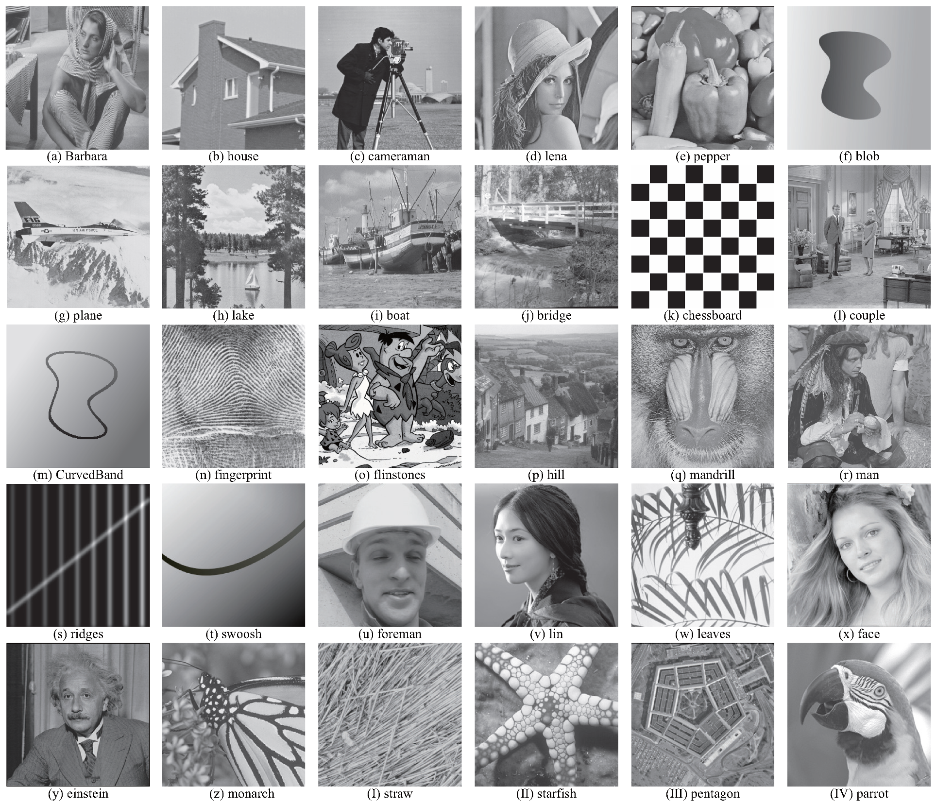
  28. Weber, A.G. The USC-SIPI Image Database: Version 5. 2006. Available online: http://sipi.usc.edu/database/ (accessed on 1 July 2022).
Figure 1. Test images.
Electronics 11 02898 g001
Figure 2. Effect of image contents on NLM smoothing parameter in terms of PSNR indices: (a) PSNR results at σ = 5 . (b) SSIM results at σ = 20 . (c) PSNR results at σ = 30 . (d) SSIM results at σ = 50 .
Electronics 11 02898 g002
Figure 3. 2D histogram of mean (E) and std (S).
Electronics 11 02898 g003
Figure 4. (a) Summed-area table. (b) Sum of a rectangular region.
Electronics 11 02898 g004
Figure 5. PSNR for image (p) with the different threshold at σ = 35 .
Electronics 11 02898 g005
Figure 6. Comparison of denoised results on the house image with σ = 30 . (a) Original image. (b) Noisy image. (c) NAMF. (d) FastHD-NLM. (e) SNN. (f) CNLM. (g) LMM-RP. (h) Proposed.
Electronics 11 02898 g006
Figure 7. Comparison of the denoising performances of different algorithms for the house image (the noise images with standard deviations σ = { 5 , 10 , 20 , 30 , 40 , 50 } ). (a) PSNR. (b) SSIM.
Electronics 11 02898 g007
Figure 8. Comparison of denoised results on the cameraman image with σ = 30 . (a) Original image. (b) Noisy image. (c) NAMF. (d) FastHD-NLM. (e) SNN. (f) CNLM. (g) LMM-RP. (h) Proposed.
Electronics 11 02898 g008
Figure 9. Comparison of the denoising performances of different algorithms for the cameraman image (the noise images with standard deviations σ = { 5 , 10 , 20 , 30 , 40 , 50 } ). (a) PSNR. (b) SSIM.
Electronics 11 02898 g009
Table 1. Comparison of experimental results on typical images based on PSNR/SSIM.
Images σ FastHD-NLMSNNCNLMLMM-RPNAMFProposed
Barbara525.63/0.9037.83/0.9638.28/0.8237.49/0.9534.13/0.8835.92/0.95
1026.40/0.8733.09/0.9234.55/0.7433.79/0.9228.12/0.7033.88/0.93
2024.83/0.8030.60/0.8530.67/0.6529.03/0.8322.13/0.4630.68/0.87
3023.55/0.7328.53/0.7728.54/0.5826.36/0.7618.72/0.3328.69/0.79
4022.47/0.6726.79/0.6926.76/0.5024.73/0.6916.38/0.2426.62/0.72
5021.88/0.6325.28/0.6125.19/0.4523.75/0.6514.65/0.1925.31/0.65
Pepper528.92/0.8937.45/0.9537.30/0.8336.79/0.9429.82/0.8734.34/0.94
1029.17/0.8731.94/0.9133.75/0.7532.99/0.9026.79/0.6932.61/0.91
2026.02/0.8129.15/0.8330.10/0.6728.76/0.8321.98/0.4429.82/0.85
3022.89/0.7227.45/0.7627.87/0.6026.08/0.7818.75/0.3227.91/0.79
4021.05/0.6525.97/0.7026.28/0.5524.19/0.7316.58/0.2426.28/0.73
5019.78/0.5924.54/0.6424.71/0.4922.86/0.6915.04/0.1925.05/0.68
Lena531.79/0.9537.84/0.9437.68/0.9437.58/0.9334.02/0.8436.63/0.93
1031.32/0.9234.00/0.8934.54/0.8934.29/0.8928.09/0.6134.63/0.90
2028.59/0.8631.48/0.8130.75/0.7830.43/0.8322.18/0.3431.61/0.84
3026.30/0.8029.52/0.7328.38/0.6728.30/0.7818.87/0.2229.61/0.77
4024.58/0.7427.96/0.6626.56/0.5626.95/0.7516.63/0.1628.13/0.76
5023.42/0.7026.59/0.6125.99/0.4926.01/0.7315.08/0.1227.06/0.75
Plane531.27/0.9138.37/0.9539.33/0.9635.70/0.9433.08/0.9037.79/0.96
1031.92/0.9033.08/0.9035.66/0.9333.94/0.9130.49/0.8534.00/0.92
2028.96/0.8530.44/0.8232.09/0.8931.07/0.8527.45/0.8329.90/0.88
3026.16/0.8128.70/0.7330.01/0.8529.04/0.8024.67/0.7730.35/0.86
4024.17/0.7727.17/0.6428.55/0.7627.51/0.7722.45/0.7328.75/0.82
5022.89/0.7425.80/0.5627.63/0.7226.34/0.7419.85/0.4827.68/0.80
Lake529.03/0.8436.04/0.9336.68/0.9435.76/0.9232.55/0.9132.39/0.91
1029.17/0.8230.28/0.8532.94/0.8631.75/0.8530.11/0.8531.14/0.88
2026.54/0.7528.26/0.7729.76/0.8027.60/0.7625.45/0.7428.81/0.82
3024.41/0.7026.91/0.7027.91/0.7225.17/0.6922.65/0.6827.99/0.78
4022.74/0.6525.63/0.6226.67/0.6923.81/0.6418.65/0.5226.68/0.67
5021.54/0.6124.46/0.5525.35/0.7022.92/0.6115.42/0.4225.60/0.61
Flinstones525.42/0.8335.52/0.9435.84/0.9535.15/0.9334.16/0.9231.32/0.91
1026.72/0.8429.89/0.8831.77/0.8931.41/0.8830.11/0.8830.19/0.89
2025.02/0.7927.10/0.8328.31/0.8227.74/0.8326.89/0.8128.35/0.85
3022.29/0.7225.98/0.7826.32/0.8024.81/0.7622.24/0.6926.46/0.80
4020.13/0.6524.80/0.7224.77/0.7422.46/0.7018.12/0.4224.81/0.75
5018.58/0.5822.70/0.6723.38/0.7020.67/0.6315.65/0.2623.53/0.69
Hill528.21/0.7935.35/0.9335.76/0.9135.52/0.9434.57/0.9331.85/0.95
1027.44/0.7429.15/0.8131.47/0.8730.46/0.8230.12/0.8030.07/0.84
2024.78/0.6227.46/0.7328.06/0.7325.99/0.6325.42/0.6828.52/0.76
3023.05/0.5326.81/0.6526.41/0.6824.06/0.5422.15/0.4226.87/0.64
4022.07/0.4724.88/0.5725.41/0.5723.10/0.4917.87/0.3625.54/0.62
5021.51/0.4423.71/0.5124.67/0.5222.58/0.4615.55/0.3024.80/0.57
Monach528.31/0.9236.30/0.9637.54/0.9736.95/0.9734.12/0.9032.68/0.96
1029.03/0.9131.84/0.9031.37/0.9432.69/0.9428.14/0.7431.31/0.94
2026.41/0.8527.35/0.7827.36/0.8928.46/0.8822.16/0.5228.81/0.88
3023.59/0.7924.70/0.6726.23/0.8525.96/0.8218.74/0.3927.05/0.82
4021.04/0.7122.84/0.5825.70/0.7024.31/0.7716.47/0.3225.63/0.77
5019.21/0.6421.25/0.5024.46/0.6722.52/0.7014.71/0.2624.63/0.71
Table 2. Performance comparison on average PSNR/SSIM.
Standard Deviations σ 51020304050
Proposed34.91/0.9633.17/0.9330.26/0.8728.20/0.8026.68/0.7525.44/0.69
NAMF34.39/0.8928.41/0.7422.49/0.5319.08/0.4116.74/0.3315.00/0.28
FastHD-NLM31.29/0.9131.09/0.8828.20/0.7925.71/0.7224.04/0.6522.98/0.61
SNN37.17/0.9632.54/0.9028.09/0.7725.51/0.6623.68/0.5722.24/0.50
CNLM38.12/0.8933.45/0.8629.58/0.8227.41/0.7825.80/0.7424.70/0.69
LMM-RP38.33/0.9734.21/0.9329.82/0.8527.29/0.7825.64/0.7324.44/0.68
Publisher’s Note: MDPI stays neutral with regard to jurisdictional claims in published maps and institutional affiliations.

