An Efficient Hyperspectral Image Classification Method: Inter-Class Difference Correction and Spatial Spectral Redundancy Removal

Abstract

Existing remote sensing images of ground objects are difficult to annotate, and building a hyperspectral dataset requires huge resources. To tackle these problems, this paper proposes a new method with low requirements for the scale of the dataset that involves correcting the inter-class differences of hyperspectral images and eliminating the redundant information of spatial–spectral features. Firstly, the algorithm introduces the spatial information of hyperspectral images into the classification task through the superpixel definition based on the entropy rate, which not only reduces the spatial redundancy information of hyperspectral images but also uses the similarity of spatial neighbors to increase the differences between classes and alleviate the differences within classes. Secondly, under the theoretical guidance of similar spectral fluctuation trends of similar objects, a feature extraction method based on fast Fourier transform is proposed to alleviate spectral feature redundancy and further eliminate the inter-class differences of the algorithm. Finally, to verify the improvement effect of the proposed idea on the traditional classification method, the idea was applied to the traditional SVM algorithm, and experiments were carried out based on the PaviaU and Indian Pines hyperspectral datasets. The simulation results show that the proposed (ERS–FFT–SVM) algorithm shows a significant improvement in classification accuracy when compared with the traditional classification algorithm and is able to perform the small sample classification of hyperspectral images.

1. Introduction

Hyperspectral images (HSIs) contain spatial information of ground objects and rich spectral information, which can provide reliable spectral fingerprint features for ground object classification tasks [1,2,3]. There are broad application prospects in all walks of life, such as crop growth assessment [4,5], mineral identification and mapping [6], and meteorological monitoring and early warning systems [7]. However, due to the differences in the reflection of different objects, the internal noise of the detector, the atmospheric correction error, and other factors, the spectral characteristics of similar objects are different, i.e., there is a phenomenon of “same object and different spectrum” in HSIs [8]. Secondly, HSIs have high-dimensional spectral features which make adjacent spectral band information similar and are, thus, prone to spectral information redundancy, “dimension disaster”, and the “Hughes phenomenon” [9]. The inter-class differences and feature redundancy of the spectral features of HSIs greatly increase the difficulty of classification. To achieve high-precision ground object classification results, large-scale labeled datasets are often required. However, with the development of hyperspectral remote sensing technology, although a large number of HSIs are easy to obtain, accurate image annotation incurs great labor and time costs [10]. Therefore, how to ensure the high-precision classification of HSIs in the case of small samples has become a research hotspot.

The spectral fingerprint features contained in HSIs can be used as the main basis for the classification of ground objects. Classical HSI classification algorithms use only spectral dimension information for classification. Among them, the K-means clustering algorithm (K-means) is one of the simplest classifiers, which considers only the Euclidean distance between training samples and test samples [11]. K nearest neighbor classification (KNN) does not require specialized training models. When there are new samples, they are compared with the training dataset, and the K nearest neighbors are found to determine the category of unknown pixels [12]. A support vector machine (SVM) can eliminate the need for a large number of training samples, and a small number of training samples can achieve good generalization ability and high classification accuracy, which can help to solve the problem of small sample learning in the classification process [13,14]. However, since these algorithms consider only the spectral information in the image and ignore the relationship between the spatial positions of different pixels, the spatial information in the image is not fully utilized, especially in the case of small samples, and the classification effect is not ideal.

With the development of hyperspectral imaging technology, the spatial resolution of HSIs is increasing, which can provide accurate ground feature information for classification tasks. At present, the method of combining spectral information and spatial information for HSI classification is receiving extensive attention. Based on spectral feature information, spatial features are introduced to make more comprehensive use of the information in HSIs [15]. Compared with single spectral feature classification, the classification accuracy of this joint feature method is significantly improved. Past studies [16,17] have introduced the method of deep learning and proposed a method of spatial–spectral feature extraction based on a deep belief network (DBN) for image classification tasks, but the huge learning network involves complex parameter selection. If the parameter selection is not appropriate, it will seriously affect the classification accuracy and computational complexity. Other researchers [18,19] have proposed an HSI classification method that combines spatial–spectral information and sparse representation. After the original image is dimensionally reduced, the local pixels on the principal component map are reorganized and sorted, and the sparse representation of the test sample of the spatial spectrum feature kernel is obtained by the supervised learning method. The extraction of spatial–spectral features via this method is relatively simple, and the sparse representation of feature information can reduce information redundancy to a certain extent. However, because the algorithm does not have special coding processing for image edge pixels, there is a phenomenon of edge misclassification, resulting in sometimes unsatisfactory classification results. Although the above spatial–spectral joint classification methods consider the use of spatial and spectral features of HSIs simultaneously, there is a substantial redundancy of feature information, leading to high computational complexity and long processing times.

In order to make up for the shortcomings of existing algorithms and the problem of low classification accuracy caused by intra-class differences and dimensional disaster in HSIs, this paper proposes an efficient ground object classification method based on an inter-class difference correction and spatial–spectral redundancy information elimination (ERS–FFT) method, and its main innovations are described as follows:

(1) This paper makes full use of the spatial information of HSIs and realizes the definition of superpixels based on the entropy rate superpixel segmentation (ERS) algorithm. Under the prior guidance that the samples contained in the superpixel are objects of the same category, the intra-class differences of the spectral features within the superpixel are corrected, and the spatial information redundancy is reduced to improve the performance of the classification algorithm.

(2) In accordance with the guidance that the fluctuation trend of spectral features of the same category of targets tends to be consistent, this paper proposes a feature extraction method based on the fast Fourier transform method. After the Fourier transformation of the spectral features, the low-frequency part represents the overall slow-changing fluctuation trend of the spectral curve, and the high-frequency part represents the fast-changing trend of the spectral curve. Extracting high- and low-frequency information to represent the fluctuation trend of spectral features can further alleviate the differences between classes.

The core objective for classification tasks with small samples is to obtain the optimal solution using the available information. SVM performs the classification task by finding the classification hyperplane and keeping the sample points in the training samples separated and as far as possible from the classification plane. For linearly indistinguishable classification problems, SVM can transform linearly indistinguishable problems in low-dimensional space into linearly separable problems in high-dimensional space by introducing kernel methods. It has good adaptability for hyperspectral datasets. The KNN classification algorithm is suitable for sample sets with many overlapping features, it is easy to operate without complicated parameter settings, but it is prone to misclassification when the number of samples is not balanced. For example, when the number of samples in a particular class is large, but the number of surrounding samples is small, this may lead to an unknown sample being classified as a large class sample when the K nearest neighbors of the sample are located more in the large class sample. Therefore, the SVM algorithm is more suitable for the problem faced in this paper, so the proposed algorithm is considered to be used in combination with SVM in this paper.

2. Proposed Algorithm

In this paper, an efficient HSI classification algorithm framework for inter-class difference correction and spatial spectrum redundancy information elimination is proposed, which is shown in Figure 1. It consists of spectral feature correction based on entropy rate superpixel segmentation, spectral curve fluctuation feature extraction, and a classical classification method (SVM). The entropy superpixel segmentation defines the superpixel block by using the spatial feature of HSI, and the spectral feature correction module uses a median filter to represent the overall spectral feature of the superpixel. The spectral curve fluctuation feature extraction uses high-frequency and low-frequency fast Fourier transform value representations. The classical classification method then achieves the final classification.

2.1. Inter-Class Difference Correction Based on Entropy Rate Superpixel Segmentation

Superpixel segmentation involves placing similar pixels in the same superpixel block. The superpixel block has boundary information, and the adjacent superpixel blocks satisfy a seamless topological relationship [20]. In the HSIs, there is a high probability that adjacent objects in space are similar. Therefore, our method uses hyper-pixel segmentation based on the entropy rate of HSIs [21,22]. By using the boundary information of hyper-pixel blocks, the subpixels in the hyper-pixel blocks of the HSIs are considered objects. The subsequent classification algorithm needs only to classify the hyper-pixel blocks to reduce the spatial redundancy information of HSI classification and improve the detection efficiency.

The input HSI can be expressed as X∈R^m×n×l, where m and n are the spatial dimensions of the HSIs, and l is the spectral segment of the HSIs. The spectral characteristics of X are analyzed by principal component analysis, and the first principal component graph X_pca∈R^m×n is obtained. A superpixel segmentation algorithm based on the entropy rate is developed for X_pca. The superpixel segmentation algorithm based on the entropy rate introduces the definition of entropy from information theory into image segmentation and performs a superpixel transformation on the image by optimizing an objective function composed of entropy rate function and balance function.

The key to a superpixel segmentation algorithm based on the entropy rate is to obtain the objective function. The objective function can be composed of the random entropy rate F(c) and equilibrium term G(c) and is expressed as Equation (1):

$$\frac{MAX}{c}\{F(c)+\lambda G(c)\}$$

(1)

where c is the edge set of image topology. Firstly, the image is initialized to obtain the graph $G=(V,E)$. The set of these vertices is V, and the set of the edges is denoted as E. By calculating the feature distance d(v_i,v_j) between pixels, the weight between vertex i and vertex j can be expressed as Equation (2):

$${\omega }_{i,j}=\exp \left\{-\frac{d{\left(v_i,v_j\right)}^2}{2{\sigma }^2}\right\}$$

(2)

The definition of the transition probability of a random walk model is shown in Equation (3):

$$P_{i,j}(A)=\left\{\begin{array}{l}\frac{{\omega }_{i,j}}{{\omega }_i}, \mathrm{if} i=j \mathrm{and} e_{i,j}\in A\hfill \\ 0, \mathrm{if} i\ne j \mathrm{and} e_{i,j}\in A\hfill \\ 1-\frac{{\displaystyle \sum _{j:e_{i,j}\in A}{\omega }_{i,j}}}{{\omega }_i}, \mathrm{if} i=j\hfill \end{array}\right.$$

(3)

where A denotes a set of combinations satisfying segmentation. Thus, the transition probability between the two vertices i and j can be obtained. According to the transition probability, F(c) and G(c) can be obtained using Equations (4) and (5):

$$F(c)=-{\displaystyle \sum _i{u}_i}{\displaystyle \sum _j{p}_{i,j}}(c)\log \left(p_{i,j}(c)\right)$$

(4)

where $u_i$ is a fixed allocation of random walk.

$$G(c)=-{\displaystyle \sum _i{p}_{z_c}}(i)\log \left(p_{z_c}(i)\right)-N_c$$

(5)

where z_c is the clustering distribution, $p_{z_c}$ is the probability of clustering distribution, and N_c is the image topology parameters. During the process of random walk, F(c) and G(c) are monotonically increasing functions with decreasing growth rates [23]. Since $\lambda$ is a positive real number, the combined function has the property of monotonically increasing with a decreasing growth rate. When the image segmentation runs according to the objective function, the segmentation ends when c equals the initial number of superpixels K.

The superpixels of the HSIs after entropy rate segmentation can be expressed as [S₁, S₂, …, S_q], where q represents the number of superpixels. The i-th superpixel S_i∈R^a×l, where a represents the number of subpixels contained in the i-th superpixel and l represents the number of spectral features of pixels. In this way, we can correct the difference in the spectral characteristics of similar targets in HSIs. The overall spectral feature HF_i∈R^l of the supernode is the result of the supernode subpixel passing through the median filter, as is shown in Equation (6), where V_ia represents the spectral feature of the a-th pixel of the i-th superpixel:

$$H{F}_i=mean(V_{i1}\hspace{1em}{V}_{i2}\hspace{1em}\dots \hspace{1em}{V}_{ia})$$

(6)

2.2. Spectral Fluctuation Feature Extraction Based on Fast Fourier Transform

Due to the high spectral dimension of HSIs, the “Hughes phenomenon” is prone to occur during classification, which leads to a significant deterioration in classification performance. In small sample classification, high-dimensional features have a more obvious influence on the final classification accuracy. The traditional spectral dimension feature extraction algorithm is designed for specific data distribution. This paper uses the fluctuation characteristics of the spectrum of the spectral curve to achieve feature extraction.

Although the spectral characteristics of the same target in HSIs are different, their fluctuation characteristics are similar. Therefore, after the fast Fourier transformation of the spectral characteristic curve, the low-frequency part of the spectrum represents the slow fluctuation trend of the target spectral characteristics, and the high-frequency part represents the rapid fluctuation trend [24]. The high-frequency and low-frequency values can be used as the extraction features of the target. The original spectral feature number of superpixels is l, assuming that the extracted feature number is k. The l-point fast Fourier transform is performed on the spectral characteristics of each superpixel, and the first k/2 low-frequency and the second k/2 high-frequency information are selected as the extraction features to realize the feature extraction process from l-dimensional to k. The extracted spectral features can be expressed as Equation (7):

$$E_i=[FFT{(H{F}_i)}_1\hspace{1em}FFT{(H{F}_i)}_2\hspace{1em}\dots \hspace{1em}FFT{(H{F}_i)}_k]$$

(7)

where k represents the k-th point after fast Fourier transform.

2.3. ERS–FFT–SVM Overall Algorithm Steps

Input: HSIs dataset X∈Rm×n×l with m × n l-dimensional data points, number of training samples $r$, number of superpixel blocks $K$   Output: Category of test samples

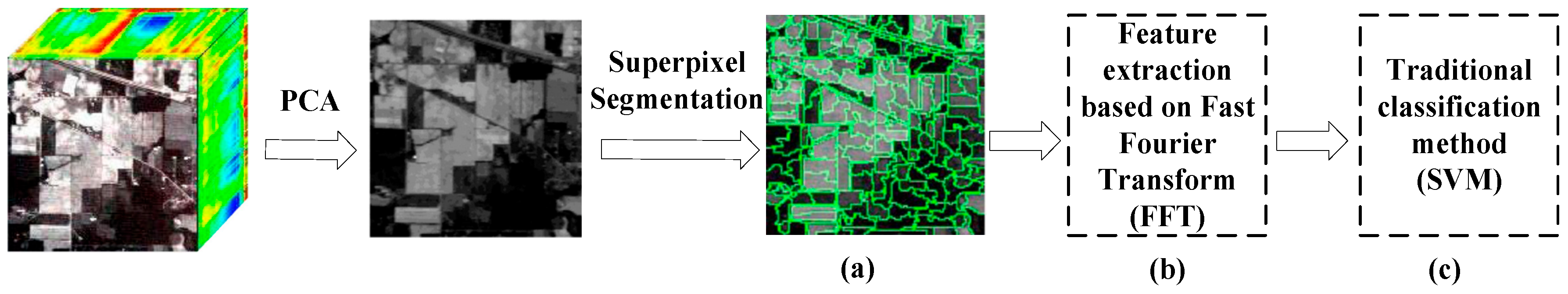
Step 1: Extract the first principal component of the high-dimensional hyperspectral data $X$ to form a two-dimensional image;   Step 2: According to the number of input superpixel blocks $K$, the image is segmented by the designed entropy-based superpixel segmentation algorithm, and $K$ superpixel blocks are obtained;   Step 3: According to the number of training samples $r$, the training samples and test samples are randomly selected from the dataset $X$, where the training sample category is known;   Step 4: Similar to the SVM algorithm, the test set is classified by the obtained $K$ superpixel blocks and the trained model.

3. Experimental Results and Analysis

3.1. Experimental Datasets

To verify the classification of the proposed algorithm in the case of small samples, the experiment in this paper was carried out on commonly used datasets, namely the PaviaU and Indian Pines datasets. The following is a brief introduction to each dataset.

• PaviaU dataset

The scene covers the University of Pavia, Italy, and the image size is 610 × 340 pixels. The dataset has a total of 103 spectral bands after removing noise. The spatial resolution of the dataset is 1.3 m, and the spectral band coverage is 0.43–0.86 microns. Pavia University has nine types of land, including natural vegetation, urban construction materials, and background. Its pseudo-color image and factual ground information are shown in Figure 2. The details of the dataset are shown in

Table 1. Features of datasets.

	Pavia University		Indian Pines
	Category	Sample Size	Category	Sample Size
1	Asphalt	6631	Alfalfa	46
2	Meadows	18,649	Corn-notill	1428
3	Gravel	2099	Corn_mintill	830
4	Trees	3064	Grass-pasture	483
5	Painted metal sheets	1345	Grass-trees	730
6	Bare Soil	5029	Grass-pasture-mowed	28
7	Bitumen	1330	Hay-windrowed	478
8	Bricks	3682	Oats	20
9	Shadows	947	Soybean-notill	972
10			Soybean-mintill	2455
11			Soybean-clean	593
12			Wheat	205
13			Woods	1265
14			Buildings-Grass-Trees-Drives	386
15			Stone-Steel-Towers	93
16			Corn	237
	Total	42,776	Total	10,249

.

The left is a pseudo-color map, and the right is a true feature category map.

2.

Indian Pines dataset

The dataset concerns a farm in northwestern Indiana collected by the spectrometer AVRIS in 1992. The image is 145 × 145 pixels, and the dataset contains 200 spectral bands. The spatial resolution of the dataset is a 20 m spectral band covering a range of 0.2–2.4 μm and containing 16 real ground object categories. Its pseudo-color image and factual ground information are shown in Figure 3, and the details are shown in Table 1.

The left is a pseudo-color map, and the right is a true feature category map.

3.2. Experiment Setting

In terms of the experimental setup to evaluate the classification performance of the proposed algorithm, the proposed algorithm was compared with KNN and SVM, which use only spectral dimension information. To achieve better results, the parameters of each algorithm are adjusted to their optima, and the nearest neighbor number selected for KNN was nine. The optimal parameters of SVM were determined by 10 cross-validations; the input parameter K of ERS–FFT–SVM was selected (from 200, 400, 600, 800, 1000, and 1200).

The evaluation indexes used in this paper include overall accuracy (OA) and the Kappa coefficient [25]. To improve the accuracy and reliability of the experiment, the average classification accuracy of each algorithm after five repetitions was calculated to obtain the final result.

3.3. Experimental Results and Analysis

Figure 4 shows the HSI classification algorithm based on the superpixel segmentation of the PaviaU dataset. For each subgraph, the abscissa axis represents the number of samples, increasing from 10 samples per class to 100 samples per class, and the ordinate axis is the overall classification accuracy of OA.

It can be seen from Figure 4b that when the number of superpixel blocks is greater than 600, the classification accuracy becomes more accurate with an increase in the number of training samples. The proposed algorithm has only 20 training samples for each type of ground object, and the OA value of the classification results can reach more than 80%. This reflects the introduction of the superpixel segmentation algorithm which combines the spatial information of HSIs and can effectively improve the classification accuracy in the case of small samples. With an increase in the number of training samples, the difference in the classification accuracy based on different superpixels is reduced. The classification accuracy is very close when the training sample is 100 and the superpixel block is 800 and 1000. This shows that as the number of training samples increases, the sensitivity of classification accuracy to the number of superpixels decreases. However, in Figure 4a, the number of superpixel blocks is 200, 400, and 600. When the training sample is greater than 80, the classification accuracy shows a downward trend because the number of superpixel blocks is too small. Usually, the greater the number of superpixel blocks, the fewer pixels are contained in each class of pixels, and when the number of superpixel blocks is small while more pixels are contained in the superpixel block, it is possible to contain multiple classes of pixel blocks in the superpixel block. In the results shown in Figure 5, the segmentation result is 1000 superpixel blocks. Each superpixel block is the same class of features, which is consistent with the assumption of the proposed algorithm that each superpixel block has the same class of pixels; thus, the number of superpixel blocks selected in this paper is 1000 to ensure the classification accuracy.

Figure 6 and Figure 7 show the classification results of PaviaU and Indian Pines when the training samples of each class are 10, 30, and 50, respectively, and the superpixel block is set to 1000. To analyze the classification results in detail,

Table 2. Overall classification accuracy and Kappa coefficient of classification algorithms under different sample numbers with the PaviaU dataset (K = 1000).

Dataset	Training Samples	KNN		SVM		ERS–FFT–SVM		OA Difference Value
		OA(%)	Kappa	OA(%)	Kappa	OA(%)	Kappa	KNN	SVM
PaviaU	10	52.7	0.4370	69.57	0.6173	75.56	0.6869	22.86	5.99
	20	62.01	0.5363	77.37	0.7099	84.44	0.7916	22.43	7.07
	30	65.03	0.5652	78.29	0.723	85.19	0.8039	20.16	6.9
	40	64.91	0.5694	79.93	0.7432	88.15	0.8427	23.24	8.22
	50	66.98	0.5935	79.99	0.7435	89.63	0.8626	22.65	9.64
	60	68.92	0.6133	81.82	0.7667	90.37	0.8722	21.45	8.55
	70	70.07	0.6363	82.42	0.7733	91.11	0.8822	21.04	8.69
	80	71.57	0.6445	82.87	0.7794	91.11	0.882	19.54	8.24
	90	71.29	0.6419	84.44	0.7989	92.59	0.9018	21.3	8.15
	100	71.97	0.6486	84.90	0.8047	93.33	0.9109	21.36	8.43
average		66.55	0.5887	80.16	0.7460	88.15	0.8437	21.6	7.99

and

Table 3. Overall classification accuracy and Kappa coefficient of classification algorithms under different sample numbers with the Indian Pines dataset (K = 1000).

Dataset	Training Samples	KNN		SVM		ERS–FFT–SVM		OA Difference Value
		OA(%)	Kappa	OA(%)	Kappa	OA(%)	Kappa	KNN	SVM
Indian Pines	10	32.79	0.2546	52.88	0.4747	57.1	0.5212	24.31	4.22
	20	44.19	0.3726	57.8	0.5293	74.2	0.711	30.01	16.4
	30	46.83	0.4030	61.1	0.5648	76.23	0.7347	29.4	15.13
	40	50.05	0.4407	65.28	0.611	78.26	0.7559	28.21	12.98
	50	53.46	0.4781	66.86	0.628	83.48	0.8146	30.02	16.62
	60	54.79	0.4929	66.86	0.6492	83.48	0.8152	28.69	16.62
	70	55.3	0.4989	70.38	0.6678	82.61	0.8054	27.31	12.23
	80	57.34	0.5216	70.51	0.6693	90.72	0.8956	33.38	20.21
	90	58.48	0.5338	72.36	0.6898	90.72	0.8958	32.24	18.36
	100	59.35	0.5438	72.85	0.6951	91.88	0.9088	32.53	19.03
average		51.26	0.454	65.69	0.6179	80.87	0.7858	29.61	15.18

provide more detailed classification OA values for training sample changes. The corresponding OA value curves are shown in Figure 8. As the number of samples increases from 10 to 100, the accuracies of different classification methods improve, which indicates that the increase in the number of samples does help to improve the classification accuracy. In addition, Figure 8 reflects that the classification accuracy using the ERS–FFT–SVM algorithm is significantly better than that of the KNN and SVM algorithms which use only spectral information. From Table 2 and Table 3, we can determine that the overall classification accuracy (OA) of ERS–FFT–SVM on the PaviaU dataset is improved by 7.99% on average compared with SVM and 21.60% on average compared with KNN in the case of small samples; in the Indian Pines dataset using ERS–FFT–SVM, accuracy is improved by 15.18% on average compared with the SVM algorithm and by 29.61% on average compared with KNN. Due to the introduction of the superpixel segmentation algorithm in the classification process, the spatial information and spectral information of HSIs are fully utilized, so the ERS–FFT–SVM algorithm shows good performance under small-sample conditions. In the experimental results with the PaviaU dataset and Indian Pines dataset, the Kappa coefficient under the ERS–FFT–SVM algorithm demonstrates that the classification results are in good agreement with the real ground objects, indicating the superior performance of the ERS–FFT–SVM algorithm.

4. Conclusions

In this paper, an efficient spatial–spectral joint classification method based on the correction of inter-class differences and the elimination of spatial–spectral redundancy information is proposed. The superpixel correction of inter-class differences is constructed by ERS and the spatial redundancy of data is reduced. The fluctuation characteristics of the spectral curve are extracted by FFT to reduce the spectral band redundancy. Finally, a complete (ERS–FFT–SVM) spatial–spectral joint classification method is performed and combined with a support vector machine, which greatly improves the classification accuracy. The experimental results with the PaviaU and Indian Pines hyperspectral datasets show that the proposed algorithm has a better classification effect and greatly improves the classification accuracy of ground objects for classification algorithms when considering only spectral dimension information. Moreover, when the training samples are scarce, the classification effect is improved significantly. When the number of samples is 10, the overall accuracy of ERS–FFT–SVM on the PaviaU dataset is 5.99% higher than that of SVM and 22.86% higher than that of KNN. The overall accuracy on the Indian Pines dataset is 4.22% higher than that of SVM and 24.31% higher than that of KNN. From the Kappa coefficient columns in Table 2 and Table 3, the Kappa coefficient values of the ERS–FFT–SVM algorithm are higher than those of the KNN and SVM algorithms for different sample numbers, which indicates that the classification results of the ERS–FFT–SVM algorithm possess a high degree of consistency with the real feature conditions.

The proposed ERS–FFT–SVM algorithm is based on the classical method of hyperspectral image classification (the SVM algorithm) and corrects the intra-class differences of spectral features within superpixels and reduces the redundancy of spatial information. Moreover, unlike traditional classification methods that use only dimensional spectral information, this algorithm considers the fusion of spatial–spectral features, resulting in a good performance in terms of classification accuracy and consistency of classification results. Especially in the case of small sample classification, the ERS–FFT–SVM algorithm still has better classification results.

However, the proposed algorithm in this paper has not yet considered the best matching relationship between the number of training samples and the number of superpixel segmentation blocks, which leads to the unstable classification performance of the algorithm. Moreover, only the combination with the SVM method has been considered, not with KNN or other classification algorithms. The subsequent work will further focus on the profound fusion of spatial–spectral features and the applicability of other classification methods, as well as clarify the relationship between the training samples and the number of superpixel segmentation blocks, to propose a classification method with better efficiency and higher classification accuracy for small-sample features. For example, if the KNN algorithm can overcome the problem of misclassification or misclassification when the number of samples is not balanced, or if it can take advantage of other algorithms, it may be able to form a more efficient and accurate classification algorithm.

References

1. Khan, M.J.; Khan, H.S.; Yousaf, A.; Khurshid, K.; Abbas, A. Modern Trends in Hyperspectral Image Analysis: A Review. IEEE Access 2018, 6, 14118–14129. [Google Scholar] [CrossRef]
2. Pei, S.; Song, H.; Lu, Y. Small Sample Hyperspectral Image Classification Method Based on Dual-Channel Spectral Enhancement Network. Electronics 2022, 11, 2540. [Google Scholar] [CrossRef]
3. Sohail, M.; Wu, H.; Chen, Z.; Liu, G. Unsupervised and Self-Supervised Tensor Train for Change Detection in Multitemporal Hyperspectral Images. Electronics 2022, 11, 1486. [Google Scholar] [CrossRef]
4. Lacar, F.M.; Lewis, M.M.; Grierson, I.T. Use of Hyperspectral Imagery for Mapping Grape Varieties in the Barossa Valley, South Australia. In Proceedings of the IGARSS 2001. Scanning the Present and Resolving the Future. In Proceedings of the IEEE 2001 International Geoscience and Remote Sensing Symposium (Cat. No.01CH37217), Sydney, NSW, Australia, 9–13 July 2001; Volume 6, pp. 2875–2877. [Google Scholar] [CrossRef]
5. Zhuang, L.; Wang, J.; Bai, L.; Jiang, G.; Sun, S.; Yang, P.; Wang, S. Cotton Yield Estimation Based on Hyperspectral Remote Sensing in Arid Region of China. Trans. Chin. Soc. Agric. Eng. 2011, 27, 176–181. [Google Scholar] [CrossRef]
6. van der Meer, F. Analysis of Spectral Absorption Features in Hyperspectral Imagery. Int. J. Appl. Earth Obs. Geoinf. 2004, 5, 55–68. [Google Scholar] [CrossRef]
7. Zhang, P.; Lu, Q.; Hu, X.; Gu, S.; Yang, L.; Min, M.; Chen, L.; Xu, N.; Sun, L.; Bai, W.; et al. Latest Progress of the Chinese Meteorological Satellite Program and Core Data Processing Technologies. Adv. Atmos. Sci. 2019, 36, 1027–1045. [Google Scholar] [CrossRef]
8. Yu, L.; Lan, J.; Zeng, Y.; Zou, J.; Niu, B. One Hyperspectral Object Detection Algorithm for Solving Spectral Variability Problems of the Same Object in Different Conditions. J. Appl. Remote Sens. 2019, 13, 026514. [Google Scholar] [CrossRef]
9. Pal, M.; Mather, P.M. Assessment of the Effectiveness of Support Vector Machines for Hyperspectral Data. Future Gener. Comput. Syst. 2004, 20, 1215–1225. [Google Scholar] [CrossRef]
10. Wang, C.; Zhang, J.; Zhang, L.; Wei, W.; Zhang, Y. Small sample hyperspectral image classification method based on memory association learning. J. Beijing Univ. Aeronaut. Astronaut. 2021, 47, 549–557. [Google Scholar] [CrossRef]
11. Boukhdhir, A.; Lachiheb, O.; Gouider, M.S. An Improved MapReduce Design of Kmeans for Clustering Very Large Datasets. In Proceedings of the 2015 IEEE/ACS 12th International Conference of Computer Systems and Applications (AICCSA), Marrakech, Morocco, 17–20 November 2015; pp. 1–6. [Google Scholar] [CrossRef]
12. Li, R.; Li, S. Multimedia Image Data Analysis Based on KNN Algorithm. Comput. Intell. Neurosci. 2022, 2022, 1–8. [Google Scholar] [CrossRef] [PubMed]
13. Fauvel, M.; Benediktsson, J.A.; Chanussot, J.; Sveinsson, J.R. Spectral and Spatial Classification of Hyperspectral Data Using SVMs and Morphological Profiles. IEEE Trans. Geosci. Remote Sens. 2008, 46, 3804–3814. [Google Scholar] [CrossRef]
14. Mounika, K.; Aravind, K.; Yamini, M.; Navyasri, P.; Dash, S.; Suryanarayana, V. Hyperspectral Image Classification Using SVM with PCA. In Proceedings of the 2021 6th International Conference on Signal Processing, Computing and Control (ISPCC), Solan, India, 7 October 2021; pp. 470–475. [Google Scholar] [CrossRef]
15. Qu, S.; Li, X.; Gan, Z. A Review of Hyperspectral Image Classification Based on Joint Spatial-Spectral Features. J. Phys. Conf. Ser. 2022, 2203, 012040. [Google Scholar] [CrossRef]
16. Guofeng, T.; Yong, L.; Lihao, C.; Chen, J. A DBN for Hyperspectral Remote Sensing Image Classification. In Proceedings of the 2017 12th IEEE Conference on Industrial Electronics and Applications (ICIEA), Siem Reap, Cambodia, 18–20 June 2017; pp. 1757–1762. [Google Scholar] [CrossRef]
17. Li, T.; Sun, J.; Zhang, X.; Wang, X. A spectral-spatial joint classification metond of hyperspectral remote sensing image. Chin. J. Sci. Instrum. 2016, 37, 1379–1389. [Google Scholar] [CrossRef]
18. Xiang-Fa, S.; Li-Cheng, J. Classification of Hyperspectral Remote Sensing Image Based on Sparse Representation and Spectral Information. J. Electron. Inf. Technol. 2012, 34, 268–272. [Google Scholar] [CrossRef]
19. Chen, Y.; Nasrabadi, N.M.; Tran, T.D. Hyperspectral Image Classification Using Dictionary-Based Sparse Representation. IEEE Trans. Geosci. Remote Sens. 2011, 49, 3973–3985. [Google Scholar] [CrossRef]
20. Liu, T.; Dai, F.; Guo, W.; Zhao, F.; Wang, J.; Wang, X. Superpixel Segmentation Algorithm Based on Local Network Modularity Increment. IET Image Process. 2022, 16, 1822–1830. [Google Scholar] [CrossRef]
21. Liu, M.-Y.; Tuzel, O.; Ramalingam, S.; Chellappa, R. Entropy Rate Superpixel Segmentation. In Proceedings of the CVPR 2011, Colorado Springs, CO, USA, 20–25 June 2011; pp. 2097–2104. [Google Scholar] [CrossRef]
22. Tang, Y.; Zhao, L.; Ren, L. Different Versions of Entropy Rate Superpixel Segmentation for Hyperspectral Image. In Proceedings of the 2019 IEEE 4th International Conference on Signal and Image Processing (ICSIP), Wuxi, China, 19–21 July 2019; pp. 1050–1054. [Google Scholar] [CrossRef]
23. Zhang, Y.; Li, X.; Gao, X.; Zhang, C. A Simple Algorithm of Superpixel Segmentation with Boundary Constraint. IEEE Trans. Circuits Syst. Video Technol. 2017, 27, 1502–1514. [Google Scholar] [CrossRef]
24. Nussbaumer, H.J. The Fast Fourier Transform. In Fast Fourier Transform and Convolution Algorithms; Nussbaumer, H.J., Ed.; Springer Series in Information Sciences; Springer: Berlin/Heidelberg, Germany, 1981; pp. 80–111. ISBN 978-3-662-00551-4. [Google Scholar]
25. Thompson, W.D.; Walter, S.D. A Reappraisal of the Kappa Coefficient. J. Clin. Epidemiol. 1988, 41, 949–958. [Google Scholar] [CrossRef]
Figure 1. Flow field diagram of general algorithm. (a) The result of superpixel segmentation. (b) FFT. (c) SVM.
Electronics 11 02890 g001
Figure 2. PaviaU dataset diagram.
Electronics 11 02890 g002
Figure 3. Indian Pines dataset diagram.
Electronics 11 02890 g003
Figure 4. Experimental results with the PaviaU dataset.
Electronics 11 02890 g004
Figure 5. Pseudo-color plot of the dataset after superpixel segmentation of 1000 blocks. PaviaU dataset on the left, Indian Pines dataset on the right.
Electronics 11 02890 g005
Figure 6. PaviaU classification results. (a) KNN. (b) SVM. (c) Proposal. (I) Training sample 10. (II) Training sample 30. (III) Training sample 50.
Electronics 11 02890 g006
Figure 7. Indian Pines classification results. (a) KNN. (b) SVM. (c) Proposal. (I) Training sample 10. (II) Training sample 30. (III) Training sample 50.
Electronics 11 02890 g007
Figure 8. OA comparison figure. (a) PaviaU. (b) Indian Pines.
Electronics 11 02890 g008