SDR-Enabled Multichannel Real-Time Measurement System for In Situ EMF Exposure Evaluation

 ,
,  ,
, 

 and
and
Abstract
:1. Introduction
2. Materials and Methods
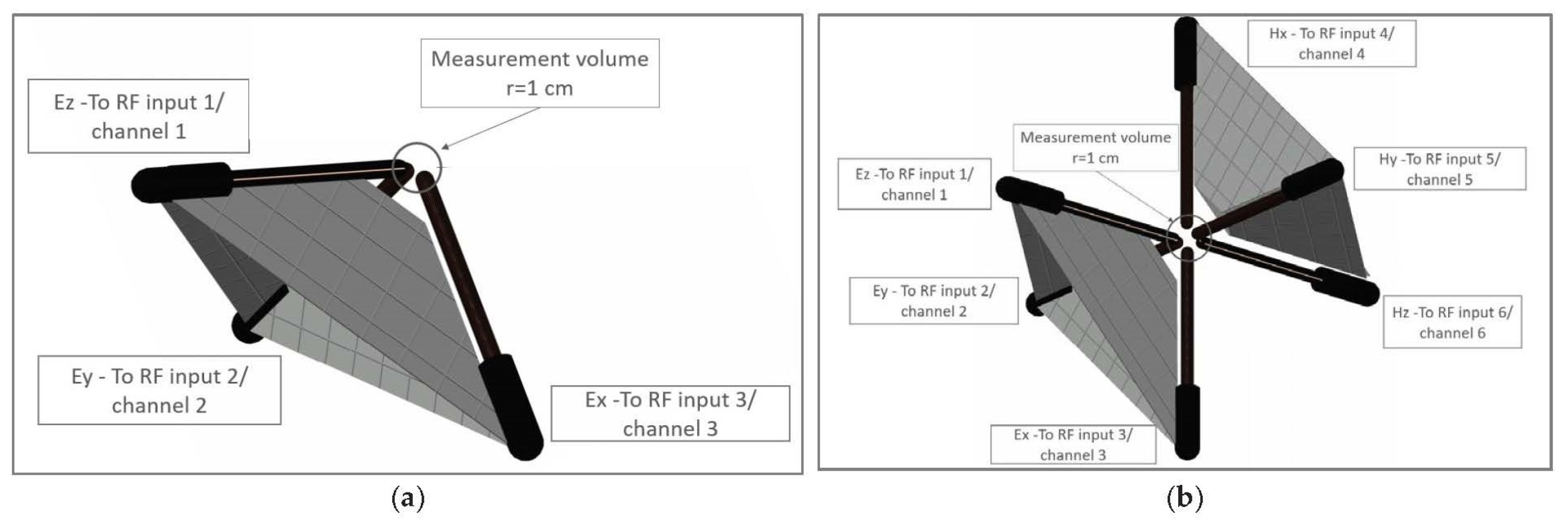
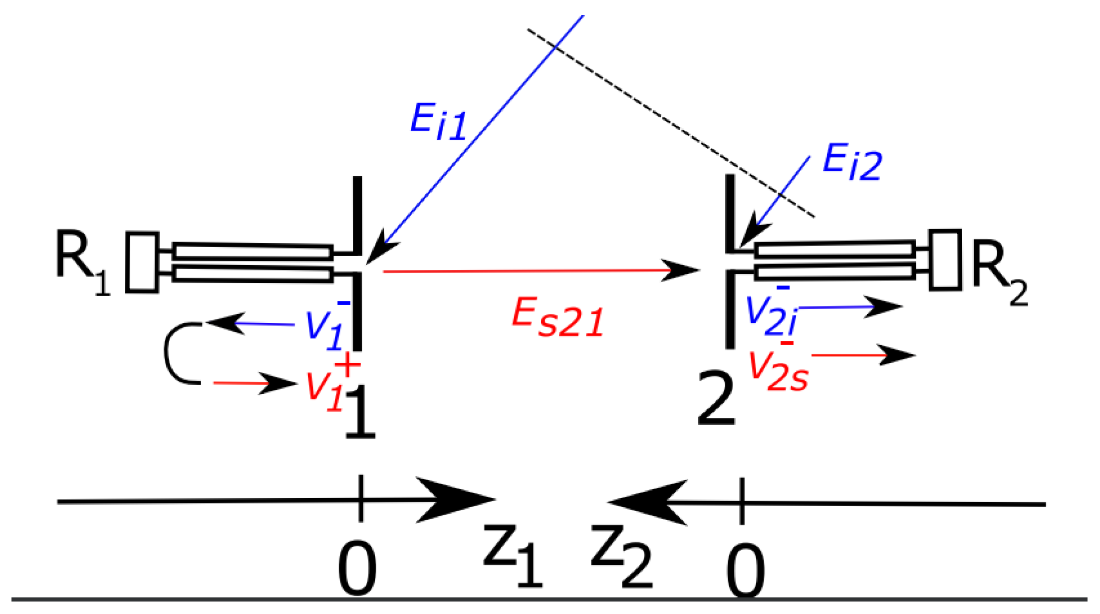
2.1. The Proposed Sensor
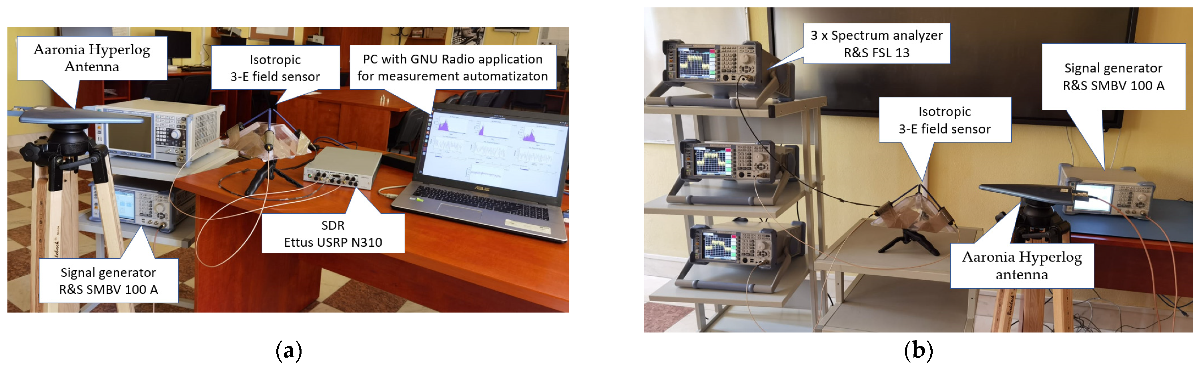
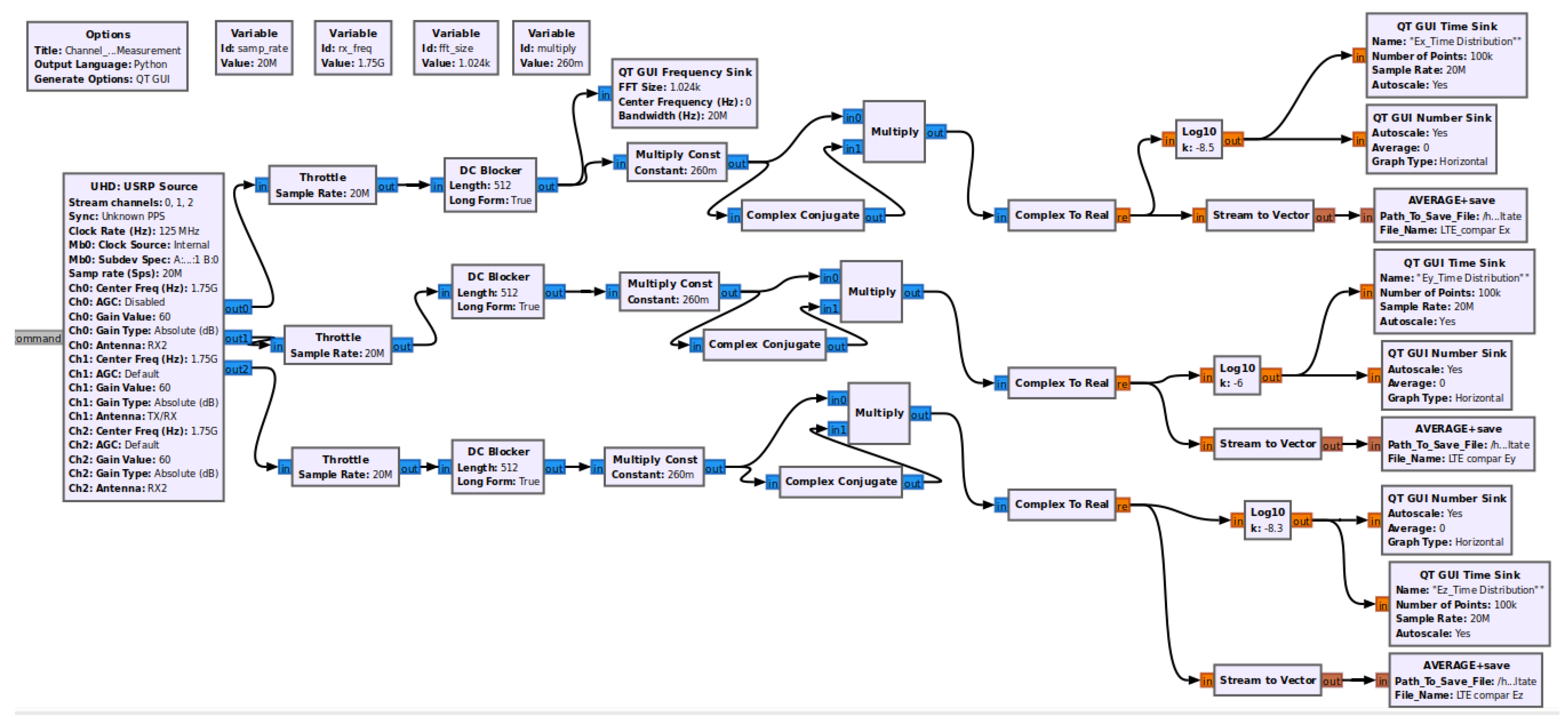
2.2. Receiver Section
- -
- file upload (large video files sent over WhatsApp)
- -
- streaming (YouTube 4k video at 720 p)
- -
- speed test (using a free available speed test app [40]).
- -
- file download—20 MHz channel bandwidth (BW)
- -
- file upload—20/40/80 MHz channel bandwidth performed by means of a free android application [41].
3. Results
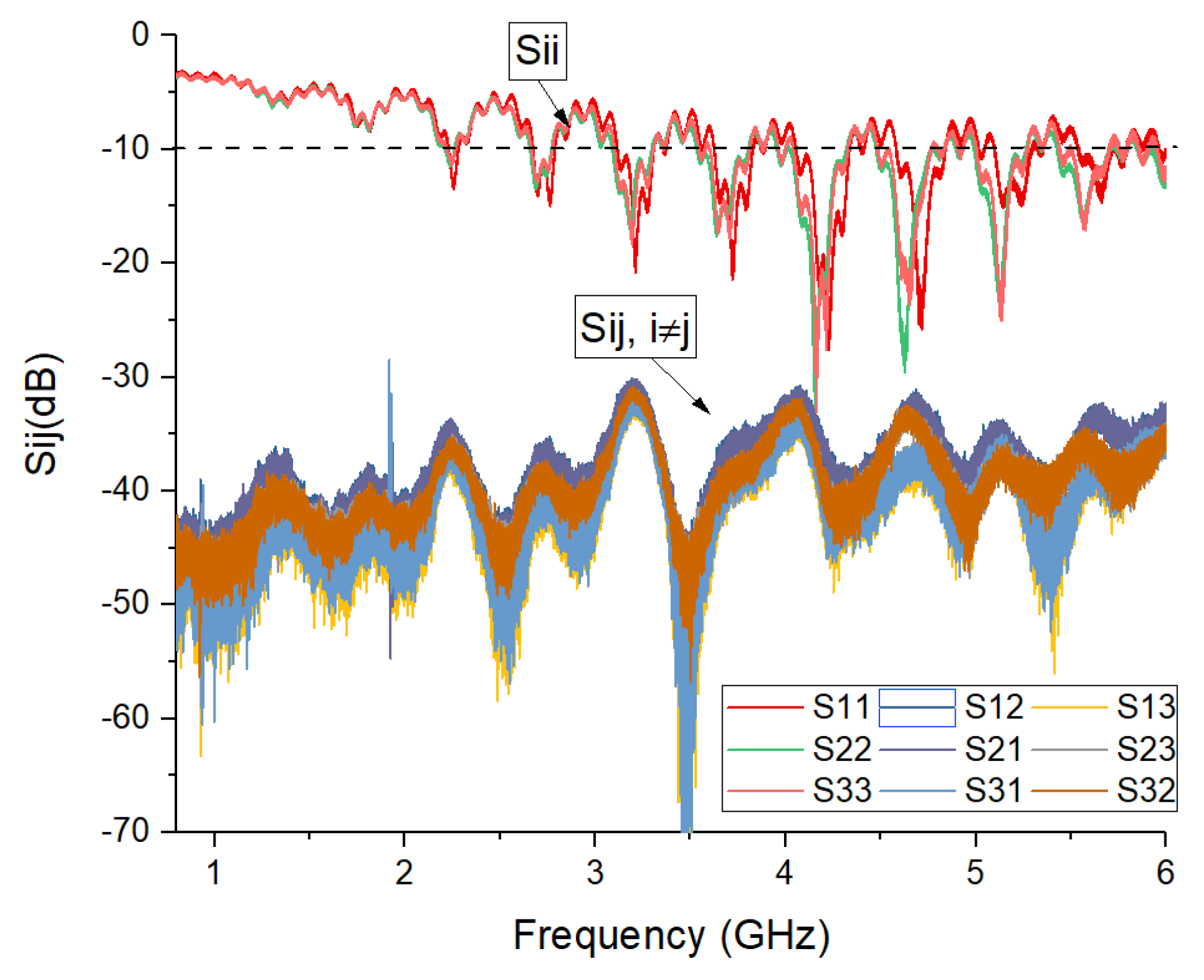
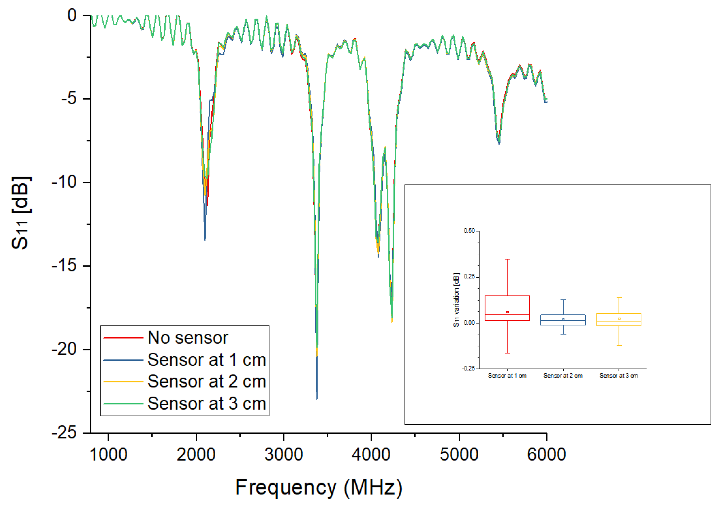
3.1. E-Field Sensor
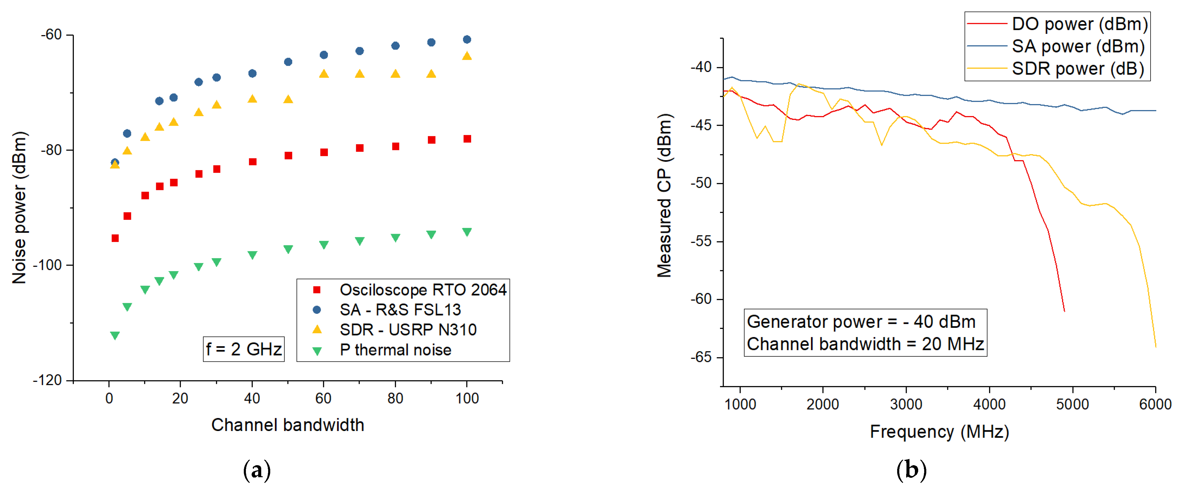
3.2. Comparative Performances of the Measurement Instruments
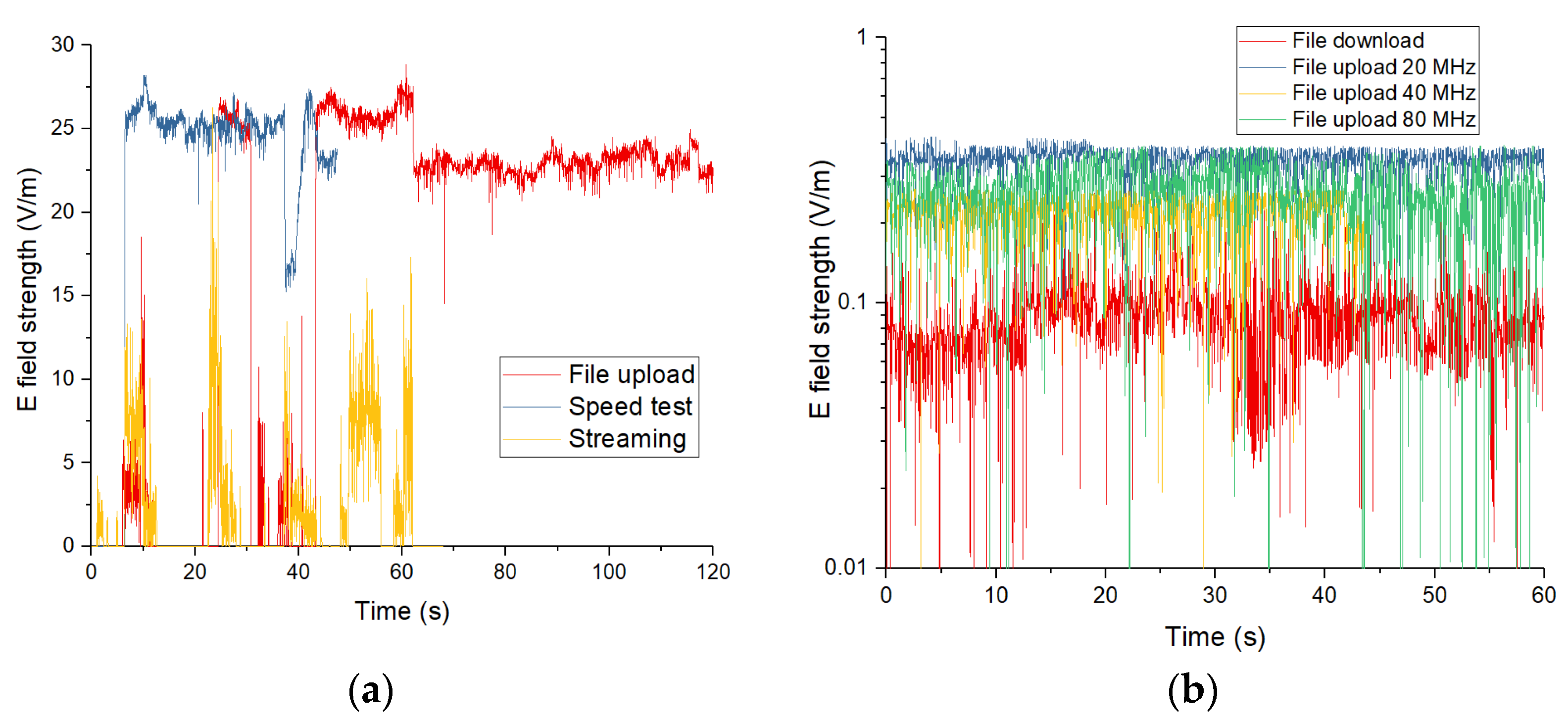
3.3. LTE-A and IEEE 802.11ax Signals Measurements
4. Conclusions
Author Contributions
Funding
Conflicts of Interest
References
- Mazar (Madjar), H. RF Human Hazards: Implementing 5G for Good: Does EMF Matter? In Proceedings of the ITU Regional Forum for Europe: 5G Strategies, Policies and Implementation, Warsaw, Poland, 22–23 October 2020.
- Aerts, S.; Verloock, L.; Bossche, M.V.D.; Colombi, D.; Martens, L.; Tornevik, C.; Joseph, W. In-situ Measurement Methodology for the Assessment of 5G NR Massive MIMO Base Station Exposure at Sub-6 GHz Frequencies. IEEE Access 2019, 7, 184658–184667. [Google Scholar] [CrossRef]
- Migliore, M.D.; Franci, D.; Pavoncello, S.; Grillo, E.; Aureli, T.; Adda, S.; Suman, R.; D’Elia, S.; Schettino, F. A New Paradigm in 5G Maximum Power Extrapolation for Human Exposure Assessment: Forcing gNB Traffic Toward the Measurement Equipment. IEEE Access 2021, 9, 101946–101958. [Google Scholar] [CrossRef]
- ICNIRP. Guidelines for limiting exposure to time-varying electric, magnetic, and electromagnetic fields (up to 300 GHz). Health Phys. 2020, 118, 483–524. [Google Scholar] [CrossRef] [PubMed]
- C95.1-2019; IEEE Standard for Safety Levels with Respect to Human Exposure to Electric, Magnetic, and Electromagnetic Fields, 0 Hz to 300 GHz. IEEE: New York, NY, USA, 2019. [CrossRef]
- Alon, L.; Gabriel, S.; Cho, G.Y.; Brown, R.; Deniz, C.M. Prospects for Millimeter-Wave Compliance Measurement Technologies [Measurements Corner]. IEEE Antennas Propag. Mag. 2017, 59, 115–125. [Google Scholar] [CrossRef]
- Schmid, T.; Egger, O.; Kuster, N. Automated E-field scanning system for dosimetric assessments. IEEE Trans. Microw. Theory Technol. 1996, 44, 105–113. [Google Scholar] [CrossRef]
- Le, D.T.; Hamada, L.; Watanabe, S.; Onishi, T. An estimation method for vector probes used in determination SAR of multiple-antenna transmission systems. In Proceedings of the 2014 International Symposium on Electromagnetic Compatibility, (EMC’14/Tokyo), Tokyo, Japan, 4–8 August 2014; pp. 629–632. [Google Scholar]
- Okano, Y.; Shimoji, H. Comparison measurement for specific absorption rate with physically different procedure. IEEE Trans. Instrum. Meas. 2012, 61, 439–446. [Google Scholar] [CrossRef]
- Gladman, A.S.; Davidson, S.R.H.; Easty, A.C.; Joy, M.L.; Sherar, M.D. Infrared thermographic SAR measurements of interstitial hyperthermia applicators: Errors due to thermal conduction and convection. Int. J. Hyperth. 2004, 20, 539–555. [Google Scholar] [CrossRef]
- Alon, L.; Cho, G.Y.; Yang, X.; Sodickson, D.K.; Deniz, C.M. A method for safety testing of radiofrequency/microwave-emitting devices using MRI. Magn. Reson. Med. 2015, 74, 1397–1405. [Google Scholar] [CrossRef]
- Miclaus, S.; Bechet, P. Estimated and measured values of the radiofrequency radiation power density around cellular base stations. Environ. Phys. 2007, 52, 429–440. [Google Scholar]
- Hodzic, V.; Gammon, R.W.; Balzano, Q.; Davis, C.C. Rapid Optical SAR Measurements; University of Maryland: College Park, MD, USA, 2016; Available online: https://www.ece.umd.edu/rrd/98-sarposterrrd09.pdf (accessed on 5 July 2022).
- Foster, K.R.; Ziskin, M.C.; Balzano, Q. Three Quarters of a Century of Research on RF Exposure Assessment and Dosimetry—What Have We Learned? Int. J. Environ. Res. Public Health 2022, 19, 2067. [Google Scholar] [CrossRef]
- Joseph, W.; Frei, P.; Roösli, M.; Thuróczy, G.; Gajsek, P.; Trcek, T.; Bolte, J.; Vermeeren, G.; Mohler, E.; Juhász, P.; et al. Comparison of personal radio frequency electromagnetic field exposure in different urban areas across Europe. Environ. Res. 2010, 110, 658–663. [Google Scholar] [CrossRef] [PubMed]
- Vallauri, R.; Bertin, G.; Piovano, B.; Gianola, P. Electromagnetic field zones around an antenna for human exposure assessment: Evaluation of the human exposure to EMFs. IEEE Antennas Propag. Mag. 2015, 57, 53–63. [Google Scholar] [CrossRef]
- Velghe, M.; Aerts, S.; Martens, L.; Joseph, W.; Thielens, A. Protocol for personal RF-EMF exposure measurement studies in 5th generation telecommunication networks. Environ. Health 2021, 20, 36. [Google Scholar] [CrossRef] [PubMed]
- Lundgren, J.; Helander, J.; Gustafsson, M.; Sjoberg, D.; Xu, B.; Colombi, D. A Near-Field Measurement and Calibration Technique: Radio-Frequency Electromagnetic Field Exposure Assessment of Millimeter-Wave 5G Devices. IEEE Antennas Propag. Mag. 2021, 63, 77–88. [Google Scholar] [CrossRef]
- Pfeifer, S.; Fallahi, A.; Xi, J.; Neufeld, E.; Kuster, N. Forward Transformation from Reactive Near-Field to Near and Far-Field at Millimeter-Wave Frequencies. Appl. Sci. 2020, 10, 4780. [Google Scholar] [CrossRef]
- Available online: https://www.anritsu.com/en-us/components-accessories/products/2000-1791-r (accessed on 9 April 2022).
- Available online: https://scdn.rohde-schwarz.com/ur/pws/dl_downloads/dl_common_library/dl_brochures_and_datasheets/pdf_1/TS-EMF_dat-sw_en_3608-9918-22_v0200.pdf (accessed on 6 July 2022).
- Available online: https://www.wavecontrol.com/rfsafety/images/data-sheets/en/WaveMon_RF-60_Datasheet_EN.pdf (accessed on 9 April 2022).
- Lipovac, A.; Lipovac, V.; Modlic, B. PHY, MAC, and RLC Layer Based Estimation of Optimal Cyclic Prefix Length. Sensors 2021, 21, 4796. [Google Scholar] [CrossRef]
- Amado, J.; Fano, G. Antenna coupling model in receiving mode. In Proceedings of the 2016 IEEE Global Electromagnetic Compatibility Conference (GEMCCON), Mar del Plata, Argentina, 7–9 November 2016; pp. 1–5. [Google Scholar] [CrossRef]
- Moraitis, N.; Popescu, I.; Nikita, K.S. Frequency Selective EMF Measurements and Exposure Assessment in Indoor Office Environments. In Proceedings of the 2020 14th European Conference on Antennas and Propagation (EuCAP), Copenhagen, Denmark, 15–20 March 2020; pp. 1–5. [Google Scholar] [CrossRef]
- Chiaramello, E.; Bonato, M.; Fiocchi, S.; Tognola, G.; Parazzini, M.; Ravazzani, P.; Wiart, J. Radio frequency electromagnetic fields exposure assessment in indoor environments: A review. Int. J. Environ. Res. Public Health 2019, 16, 955. [Google Scholar] [CrossRef]
- Jomaa, K. Electromagnetic Near-Field Characterization & Occupational Exposure to RF Waves in Industrial Environment. Ph.D. Thesis, Université Grenoble Alpes, Saint-Martin-d’Hères, France, 2018. [Google Scholar]
- Sârbu, A.; Bechet, P.; Miclăuș, S.; Helbet, R.; Șorecău, E. Isotropic near field measurement system for new generation communication signals: Preliminary design and USRP calibration. In Proceedings of the 2021 International Conference on Applied and Theoretical Electricity (ICATE), Craiova, Romania, 27–29 May 2021; pp. 1–5. [Google Scholar] [CrossRef]
- Helbet, R.; Bechet, P.; Monda, V.; Miclaus, S.; Bouleanu, I. Low-Cost Sensor Based on SDR Platforms for TETRA Signals Monitoring. Sensors 2021, 21, 3160. [Google Scholar] [CrossRef]
- Available online: https://aaronia.com/antennas/rf-and-near-field-probes/ (accessed on 3 April 2022).
- Balanis, C.A. Antenna Theory, Analysis and Design, 1st ed.; John Wiley & Sons: New York, NY, USA, 1982. [Google Scholar]
- Collin, R.E. Foundations for Microwave Engineering, 2nd ed.; Wiley-IEEE Press: New York, NY, USA, 2000. [Google Scholar]
- Perotoni, M.B.; Silva, L.A.; Silva, W.; Santos, K.M.G. Near-Field Measurement System Based on a Software Defined Radio. Prog. Electromagn. Res. Lett. 2022, 102, 87–94. [Google Scholar] [CrossRef]
- Abbas, Y.M.O.; Asami, K. Design of Software-Defined Radio-Based Adaptable Packet Communication System for Small Satellites. Aerospace 2021, 8, 159. [Google Scholar] [CrossRef]
- Armas Jiménez, S.; Sanchez-Garcia, J.; Castillo-Soria, F.R. Self Interference Cancellation on a Full Duplex DFTs-OFDM System using GNU Radio and USRP. IEEE Lat. Am. Trans. 2021, 19, 1781–1789. [Google Scholar] [CrossRef]
- Avuthu, A.R.; Battula, R.B.; Gopalani, D. An efficient spectrum sensing over η-μ fading on sub 6 GHz bands: A real-time implementation on USRP RIO. Wirel. Netw. 2022, 28, 2567–2577. [Google Scholar] [CrossRef]
- Cao, K.; Jiang, M.; Gao, S. Spectrum availability prediction based on RCS-GRU model. Phys. Commun. 2021, 49, 101479. [Google Scholar] [CrossRef]
- Zhang, L.; Lin, C.; Yan, W.; Ling, Q.; Wang, Y. Real-Time OFDM Signal Modulation Classification Based on Deep Learning and Software-Defined Radio. IEEE Commun. Lett. 2021, 25, 2988–2992. [Google Scholar] [CrossRef]
- Bechet, A.C.; Helbet, R.; Bouleanu, I.; Sarbu, A.; Miclaus, S.; Bechet, P. Low Cost Solution Based on Software Defined Radio for the RF Exposure Assessment: A Performance Analysis. In Proceedings of the 2019 11th International Symposium on Advanced Topics in Electrical Engineering (ATEE), Bucharest, Romania, 28–30 March 2019. [Google Scholar] [CrossRef]
- Available online: https://consumer.huawei.com/uk/community/details/App-Gallery-Speedtest-by-Ookla/topicId_38770/ (accessed on 5 July 2022).
- PZolee’s Blog. Available online: http://pzoleeblogen.wordpress.com/2013/11/26/wifi-speed-test-for-androidhow- (accessed on 5 July 2022).
- Paljanos, A.; Miclăuș, S.; Bechet, P.; Munteanu, C. Assessment of mobile phone user exposure to UMTS and LTE signals: Comparative near-field radiated power levels for various data and voice application services. J. Electromagn. Waves Appl. 2016, 30, 1101–1115. [Google Scholar] [CrossRef]


| No. | Communication Standard | Scenario | Channel’s Central Frequency (MHz) | Channel’s Bandwidth (ChBw) (MHz) |
|---|---|---|---|---|
| 1 | LTE-A | File upload | 1750 | 20 |
| 2 | LTE-A | Streaming | 1750 | 20 |
| 3 | LTE-A | Speed test | 1750 | 20 |
| 4 | IEEE 802.11ax | TCP Download | 5220 | 20 |
| 5 | IEEE 802.11ax | TCP Upload | 5220 | 20 |
| 6 | IEEE 802.11ax | TCP Upload | 5230 | 40 |
| 7 | IEEE 802.11ax | TCP Upload | 5210 | 80 |
| Criteria | SDR-Enabled Measurement System | SA-Enabled Measurement System | DO-Enabled Measurement System | |
|---|---|---|---|---|
| Hardware requirements |
|
|
| |
| Software requirements | GNU Radio (open source) application | Python application for remote control process | Python application for remote control process | |
| Flexibility | Medium | Reduced | Medium | |
| Performance | DANL | Good | Good | Best |
| Accuracy | Good, can be improved if previously calibrated | High | Good but limited to sub 4 GHz frequency range | |
| Cost (Euro) | 17,000 | 63,500 | 33,500 | |
Publisher’s Note: MDPI stays neutral with regard to jurisdictional claims in published maps and institutional affiliations. |
© 2022 by the authors. Licensee MDPI, Basel, Switzerland. This article is an open access article distributed under the terms and conditions of the Creative Commons Attribution (CC BY) license (https://creativecommons.org/licenses/by/4.0/).
Share and Cite
Sârbu, A.; Migliore, M.D.; Șorecău, E.; Șorecău, M.; Miclăuș, S.; Bechet, P. SDR-Enabled Multichannel Real-Time Measurement System for In Situ EMF Exposure Evaluation. Electronics 2022, 11, 2670. https://doi.org/10.3390/electronics11172670
Sârbu A, Migliore MD, Șorecău E, Șorecău M, Miclăuș S, Bechet P. SDR-Enabled Multichannel Real-Time Measurement System for In Situ EMF Exposure Evaluation. Electronics. 2022; 11(17):2670. https://doi.org/10.3390/electronics11172670
Chicago/Turabian StyleSârbu, Annamaria, Marco Donald Migliore, Emil Șorecău, Mirela Șorecău, Simona Miclăuș, and Paul Bechet. 2022. "SDR-Enabled Multichannel Real-Time Measurement System for In Situ EMF Exposure Evaluation" Electronics 11, no. 17: 2670. https://doi.org/10.3390/electronics11172670
APA StyleSârbu, A., Migliore, M. D., Șorecău, E., Șorecău, M., Miclăuș, S., & Bechet, P. (2022). SDR-Enabled Multichannel Real-Time Measurement System for In Situ EMF Exposure Evaluation. Electronics, 11(17), 2670. https://doi.org/10.3390/electronics11172670