Application of Generative Adversarial Network and Diverse Feature Extraction Methods to Enhance Classification Accuracy of Tool-Wear Status

Abstract

The means of accurately determining tool-wear status has long been important to manufacturers. Tool-wear status classification enables factories to avoid the unnecessary costs incurred by replacing tools too early and to prevent product damage caused by overly worn tools. While researchers have examined this topic for over a decade, most existing studies have focused on model development but have neglected two fundamental issues in machine learning: data imbalance and feature extraction. In view of this, we propose two improvements: (1) using a generative adversarial network to generate realistic computer numerical control machine vibration data to overcome data imbalance and (2) extracting features in the time domain, the frequency domain, and the time–frequency domain simultaneously for modeling and integrating these in an ensemble model. The experiment results demonstrate how both proposed modifications are reasonable and valid.

1. Introduction

Tool management for computer numerical control (CNC) has long been a topic of focus for manufacturers. Tools are worn down as they are used. Below a certain degree of wear, they can still function normally. However, once the wear reaches the threshold, it will no longer function normally and may even damage the products. Manufacturers must therefore carefully monitor tool wear in CNC machinery and replace the tools when the extent of wear approaches the threshold. In the past, the timing at which tools should be replaced was difficult to determine. Manufacturers mainly had to rely on the experience of onsite personnel, who determined the timing based on the sound of cutting or the statuses of the previously processed product. This approach is inconvenient: an experienced worker must be monitoring the machinery at all times during operation, and even then, tools may be replaced too early or too late. The former means discarding tools when they can still be used, which is a waste of resources. The latter may result in damaged products, which reduces the yield and incurs additional costs. To avoid these issues, researchers have developed the Prognostics and Health Management guidelines [1,2,3] to assist factories in predicting and managing the health status of machines. This framework comprises the six following steps: data processing, feature extraction, diagnostics, prognostics, decision support, and feedback and learning. Among these, diagnostics (identification of tool wear state) and prognostics (prediction of remaining tool life) are the most frequently discussed. These two steps are key to the success of analysis, as it is impossible to manage the status of machines if these two steps are not executed well. Both diagnostics and prognostics are significantly influenced by variables such as the machine type, tool type, and environment. In this study, we focus on diagnostics, which we define as directly determining the wear status of a tool (i.e., rapid initial wear, uniform wear, or failure wear) based on vibration or sound data (see Figure 1).

Most existing methods for tool wear analysis employ various sensors such as vibration sensors, acoustic emission sensors, and torque sensors to collect data from machine operations. Then, relevant information called features is extracted from the collected data. The features are input into various machine learning models for modeling [4,5]. For example, Chen et al. [6] used a logistic regression-based model to analyze the vibration signals for monitoring the statuses of tools. Kong et al. [7] proposed a Gaussian process regression model to predict the wear of the tool. Benkedjouh et al. [8] used multiple sensors to collect data and used these data to understand the health of cutting tool. Cai et al. [9] proposed a proportional covariate model for analyzing the vibration signals and thus monitored the reliability of the tools. Zhu and Liu [10] and Yu et al. [11] applied the Markov-model-based method to monitor the tool wear and predict the statuses of tools, respectively. Later, some deep learning models were developed to assess the statuses of tools during the manufacturing process. For example, Kurek et al. [12] employed a convolutional neural network to analyze the drill wear. Rohan et al. [13] used convolutional neural networks to detect and diagnose the faults of an industrial robot. To predict tool wear, Zhang et al. [14] used a long short-term memory model, whereas Cao et al. [15] combined derived wavelet frames with a convolutional neural network. In contrast, Sun et al. [5] utilized an auto-encoder method. Chen et al. [16] designed a framework based on the radial basis function and deep recurrent neural networks to swiftly generate lightweight models for the prediction of tool lifespan.

The researchers above all claimed that their approaches could successfully analyze tool-wear status and lifespan. However, we found that most of these studies focused on model development and neglected two fundamental issues in machine learning: data imbalance and feature extraction. The quantity of data for the three tool-wear statuses (i.e., rapid initial wear, uniform wear, and failure wear) will always be imbalanced. For example, in Figure 1, the quantities of the tool-wear statuses in descending order are uniform wear > failure wear > rapid initial wear. In practice, data on failure wear are even less, as tools are replaced as soon as failure wear is detected. Therefore, most manufacturers will only have access to the datasets featuring data imbalance. Few studies have addressed this topic. Carino et al. [17] proposed using incremental learning to debug data imbalance for the friction test. Brito et al. [18] suggested using unsupervised artificial intelligence techniques to improve the identification of imbalanced datasets while Miao et al. [19] proposed using deep supervision to introduce a surrogate loss function based on the Matthews correlation coefficient. Similarly, Rohan [13] and Rohan et al. [20] proposed using a generative adversarial network model with robotic arms. However, the methodology proposed by [13,17,20] is not specifically designed for tool wear, and while the methodology proposed by [18,19] is applicable to tool wear, its solution is limited to a specific model, which is not generalizable. The current paper therefore proposes a novel approach to data imbalance that is widely applicable. With regard to feature extraction, most algorithms only implement a single feature extraction method, such as one that only considers the features of tool-wear data in the time domain, the frequency domain, or the time–frequency domain. However, whether a single feature extraction method can completely extract features crucial to tool-wear status remains undetermined. This is not only because the features of wear data generated by different CNC machines may differ, but also because the features of wear data generated by the same CNC machine may also vary significantly with the workpiece. The features of wear data from different wear statuses may also vary. For some wear statuses, time features may be better classified in the time domain; for other wear statuses, the frequency or time–frequency domain may be required. Thus, we propose that multiple feature extraction methods are imperative in modeling tool wear.

This study proposes two approaches to overcome the aforementioned issues: (1) using a generative adversarial network (GAN) to generate data to overcome data imbalance and (2) extracting three types of features in the target algorithm and integrating these in an ensemble model. With regard to the first approach, GANs are a type of deep learning model in the field of artificial intelligence. They use two deep learning networks, namely a generator and a discriminator, that learn from each other to generate realistic data. The generator receives input comprising a set of vectors and then creates data that have features similar to those of historical data, whereas the discriminator determines whether the data generated by the generator are realistic. During the training process, the generator and the discriminator are continuously trained to outperform the other; the better the generator is at creating realistic data, the better the discriminator must become at identifying fake data. After a series of rounds, the features of the data produced by the generator become increasingly similar to those of historical data, thereby achieving the objective of the GAN. The GAN has been widely applied to various topics involving data generation. For instance, Goodfellow [21] designed a basic GAN framework to generate real-looking handwritten numbers and human faces. Karras et al. [22] proposed a novel progressive GAN and verified that it can greatly improve human face generation. Yadav et al. [23] developed a cyclic synthesized attention-guided GAN to further optimize virtual human face generation. Shi et al. [24] designed a GAN that transforms 2D human face images into 3D images. Fang et al. [25] developed a GAN to produce human faces from human speech fragments. Chen et al. [26] proposed a GAN that uses two discriminators at the same time to repair images. Wei et al. [27] presented an occlusion-aware warping GAN to overcome the issue of blocked human images in videos. In addition to human face recognition, a number of recent studies have applied GAN to generate manufacturing data. For example, Tagawa et al. [28] used a GAN to reconstruct sound signals and detect abnormalities in noisy factory environments. Zhang et al. [29] proposed a multi-view GAN to generate images of real vehicles from skeleton views. Gan et al. [30] employed a GAN to enhance the detection rates of an automatic leather patch defection system. Gu et al. [31] utilized a conditional GAN to generate samples of rolling bearing failures and thereby enhance the accuracy of detecting failure based on vibration signals from rolling bearings. In the current paper, we applied a GAN to generate realistic CNC machine operating data (including vibration signals and sound signals) to resolve data imbalance.

In terms of feature extraction, we surveyed relevant studies to identify the three domains most commonly employed for modeling: the time, frequency, and time–frequency domains. We established a deep learning model for each type of extracted feature and then employed an ensemble learning model to integrate the results. We postulated that extracting various types of features will offer an advantage in tool-wear status classification by processing wear problems comprehensively.

In our framework, we first cleaned the collected data and used a GAN to produce additional operating data. Then, we obtained features from the time, frequency, and time–frequency domains. Third, we used three deep learning models to model the three types of features; the output of each model was the classification of the current tool-wear status as rapid initial wear, uniform wear, or failure wear. Finally, we used an ensemble learning model to integrate the results of the three models to output the current tool-wear status to the user. We conducted several experiments to verify the performance of the proposed approaches.

The remainder of this paper is structured as follows. Section 2 introduces relevant literature on tool wear and Section 3 outlines the framework of the proposed approaches. Section 4 presents our experiment simulations and Section 5 contains the conclusion and directions for future work.

2. Related Work

This chapter reviews three important topics: (1) tool-wear statuses; (2) data fields suitable for tool wear predictions; and (3) existing tool wear prediction methods.

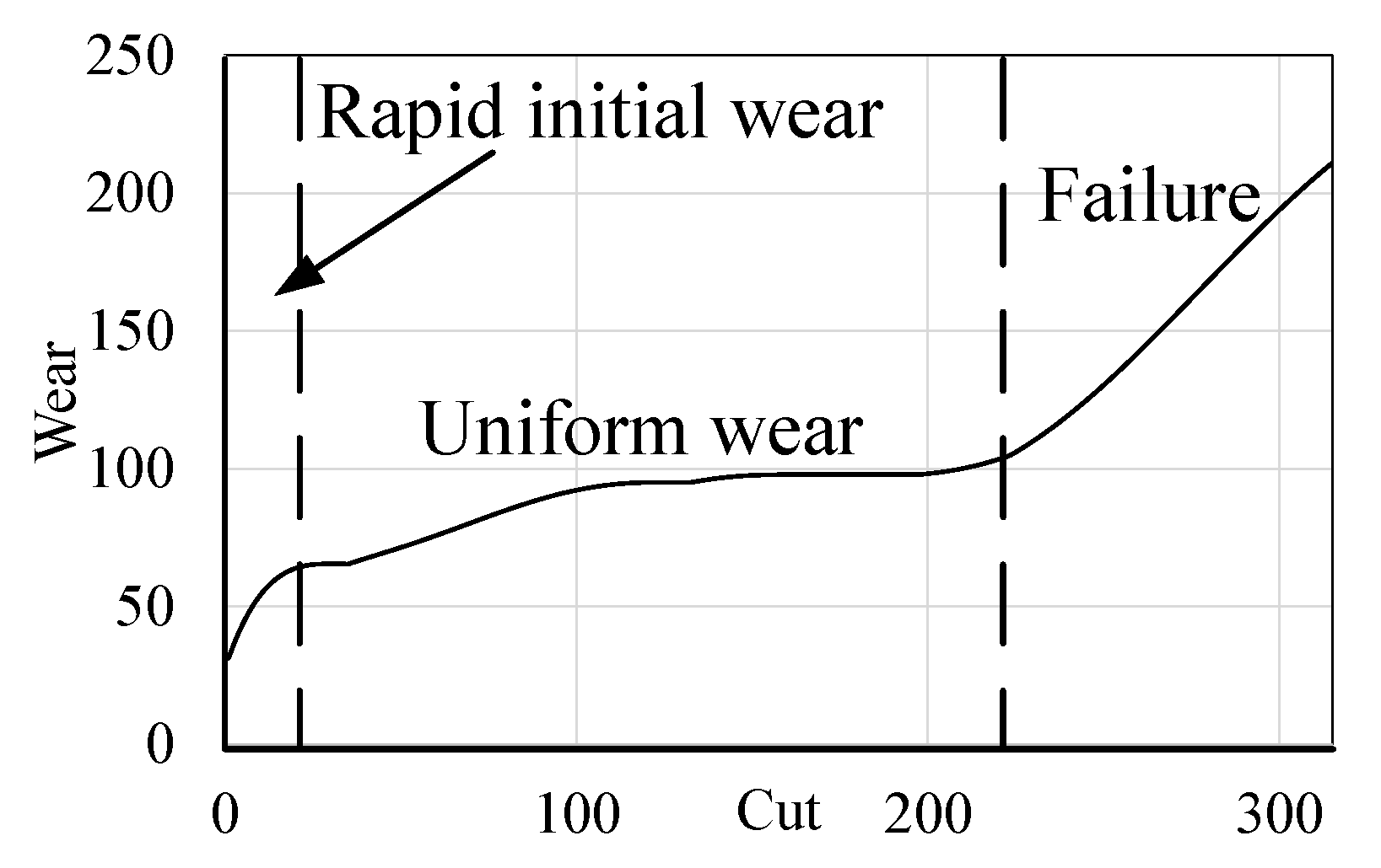
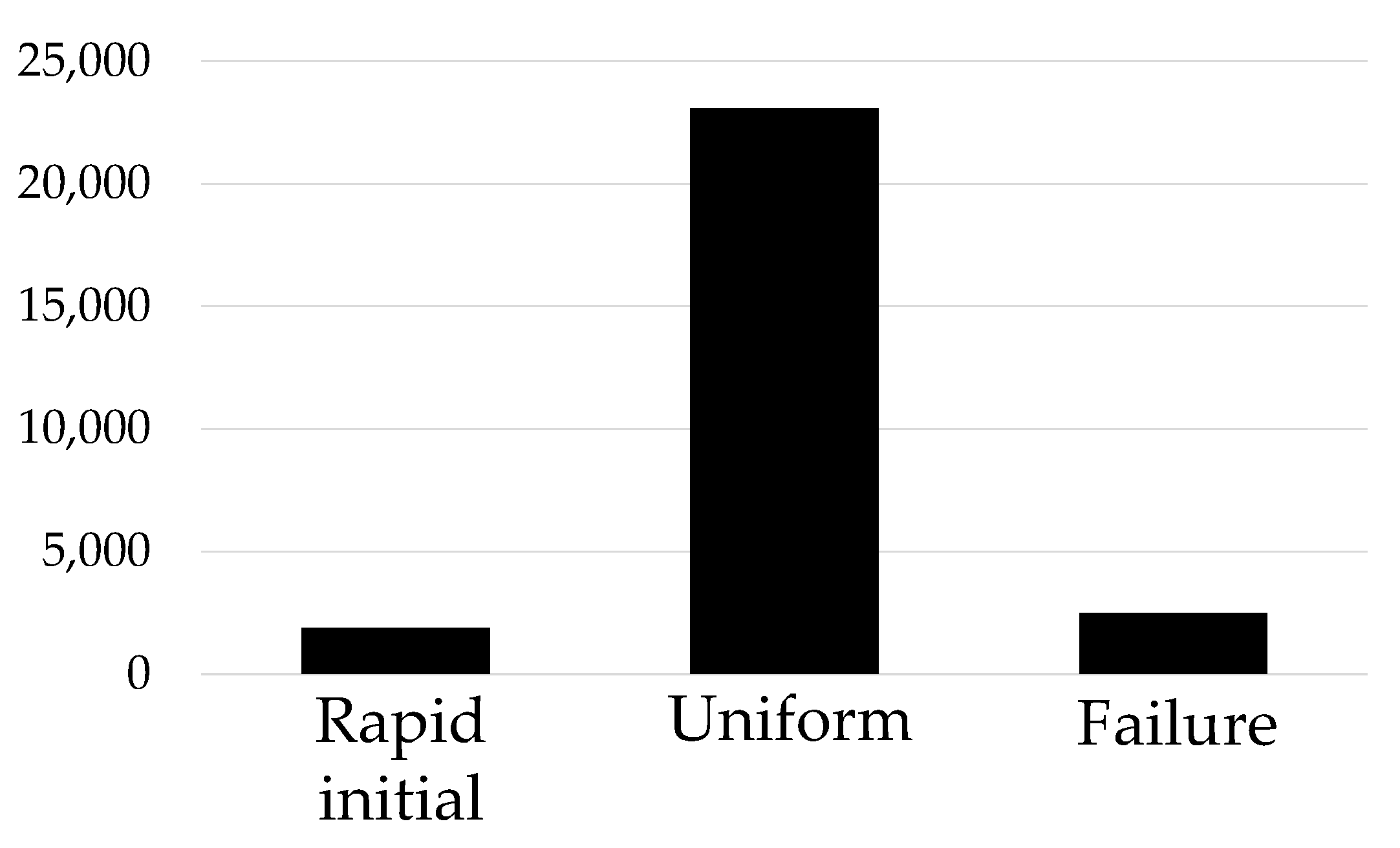
2.1. Tool-Wear Statuses

Tool wear can be divided into three phases [32]: rapid initial wear, uniform wear, and failure. These are depicted in Figure 1. In the first phase, tool blades may not be of uniform lengths and blade edges are very sharp. Thus, wear in this phase is rapid. In the second phase, differences in tool length have evened out, creating a larger area to bear force, which reduces the pressure. Thus, wear in this phase is slower and steadier, with no sharp fluctuations. In the final phase, the tool has become blunt, thereby increasing the cutting resistance, required cutting power, and cutting temperature. The wear rate therefore significantly increases, and the probability of failure is high. In practice, tools are replaced before they reach this phase to protect process quality. To achieve consistency and comparability in tool-wear judgment, ISO 8688-2 suggests that tools should be replaced if the average wear of multiple tools exceeds 0.3 mm or if the wear of a single tool exceeds 0.5 mm [33].

2.2. Data Fields Suitable for Tool Wear Predictions

Researchers have demonstrated which data fields can be used to effectively predict tool-wear statuses; these include sound, vibrations, and electric currents. For instance, Erturk et al. [34] indicated that process parameters such as cutting speed, cutting time, and cutting depth all exert influence on tool wear. Bhuiyan et al. [35] utilized an acoustic emission sensor to collect the soundwave signals produced by a cutting tool to analyze tool-wear statuses. Dolinsek et al. [36] similarly used an acoustic emission sensor to examine the relationship between tool-wear statuses and workpiece material. Bhuiyan et al. [37] speculated that when tools become dull, the rotational speed slows down, causing the machine to increase its electrical current to reach the required speed. They therefore used the relationship between the rotational speed and electrical current to predict tool wear. In recent years, a number of studies have used vibration signals to predict tool wear [6,9]. Despite good results, some researchers insist that a single sensor fails to provide a comprehensive evaluation of tool wear. For example, Benkedjouh et al. [8] used acoustic emission sensors, accelerometers, and force sensors to collect data on tool wear.

2.3. Existing Tool Wear Prediction Methods

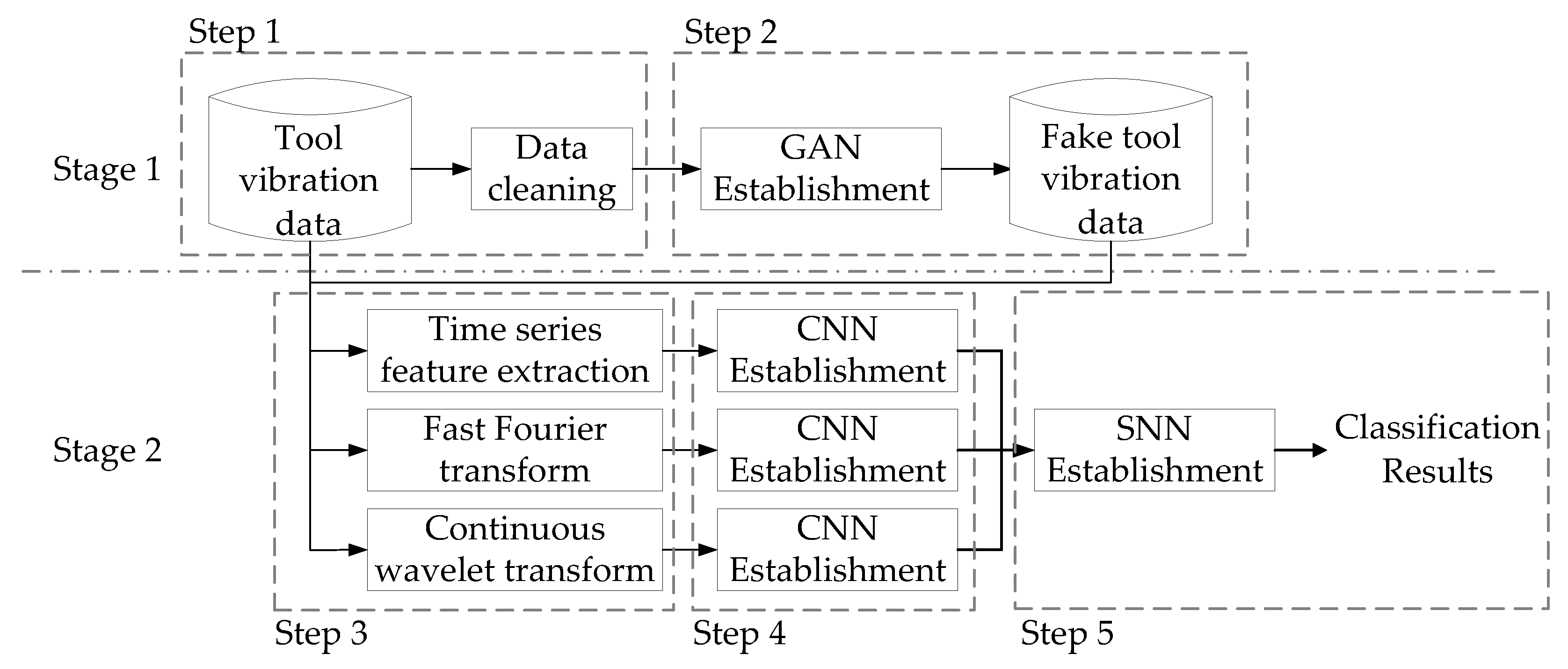
Approaches to tool wear prediction research can be divided into two categories: early machine-learning methods and recent deep-learning methods. The former approach has been widely applied in a range of contexts. Li et al. [38] used a random forest and a multiple linear regression model to analyze vibration signals. Kong et al. [7] proposed a novel Gaussian regression model. Cai et al. [9] proposed a proportional covariate model for vibration signals. Gomes et al. [39] employed a support vector machine to analyze the vibration data from milling manufacturers. Mohanraj et al. [40] also used a support vector machine for milling data but included a decision tree for feature selection to increase the monitoring accuracy. Jalali et al. [41] used a support vector machine to monitor the ball bearing failure with a genetic algorithm for feature selection. Markov models and artificial neural networks are also popular. For instance, Zhu and Liu [10] and Yu et al. [11] utilized a Markov model to predict the tool statuses, while Corne et al. [42] and Hesser et al. [43] used artificial neural networks to, respectively, monitor drilling processes and tool wear.

The emergence of DLMs brought increased accuracy to tool wear predictions. Zhang et al. [14] and Zhao et al. [44] used LSTM models to monitor machine health. Kurek et al. [12] analyzed the drill head wear using a convolutional neural network. Cao et al. [15] and Cheng et al. [45] first applied the wavelet transform to sound or vibration signals and then input the results into a convolutional neural network. Other examples include Sun et al. [5], who used an auto-encoder method, and Zhao et al. [46], who employed a gated recurrent unit-based approach to perform the gear and shaft malfunction detection. These studies demonstrate the superiority of DLMs over conventional machine learning.

3. Frameworks

The framework in this paper is divided into two stages, as shown in Figure 2. In the first stage, collected tool vibration data are cleaned using linear interpolation to fill in the missing values and the data are organized into a temporal matrix format to serve as GAN input. This represents Step 1. In Step 2, the GAN model is established and trained to solve the common data imbalance issue in tool-wear problems. The second stage includes Step 3, in which three different methods are employed to obtain the features of tool-wear status classifications and solve the problem of the unsuitability of single-classification feature selection methods for all tool-wear problems. In Step 4, a convolutional neural network (CNN) is established and trained for each feature selection method to classify the tool-wear status. The final step of the second stage is Step 5, in which a shallow neural network (SNN) is used to perform ensemble learning with the outputs of the three CNNs established in the previous step. Below, we describe all five steps in detail.

3.1. Introduction to the Dataset and the Methods for Data Cleaning

The dataset used in this study was from the 2010 PHM Data Challenge [16,47]. It contains data collected during cutting using a CNC machine, with a sensor data collection rate of 50 k/Hz, 6 mm ball nose tungsten carbide cutters, and HRC52 stainless steel workpieces. The parameters of the machine-cutting experiment were a spindle speed of 10,400 RPM, a feed rate of 1555 mm/min, and a cutting depth of 0.2 mm. Data were included from six cutters. The organizers of the challenge selected three of the six cutters as training sets and provided the wear value after each cut as well as the vibration data from the cutting processes. The data from the three remaining cutters served as test sets. For these cutters, the wear values after each cut were not provided, so we only employed the three datasets serving as training sets in this study.

Each cutter was used to make 315 cuts, and for each cut, various features were recorded, as shown in

Table 1. Dataset from 2010 PHM data challenge.

	Acceleration in x Axis	Acceleration in y Axis	Acceleration in z Axis	x Vibrations	y Vibrations	z Vibrations	Acoustic Emission
1	0.704	−0.387	−1.084	0.018	0.031	0.027	−0.004
2	0.772	−0.573	−1.153	−0.056	−0.057	−0.058	−0.004
3	0.828	−0.673	−1.242	0.037	0.019	0.031	−0.004
…	…	…	…	…	…	…	…
127,399	0.207	0.483	0.292	0.111	0.114	0.125	−0.004

. The seven columns in the table present acceleration in the x axis, acceleration in the y axis, acceleration in the z axis, vibration in the x axis, vibration in the y axis, vibration in the x axis, and acoustic emission. As the cutting time varied with each cut, the quantity of data collected ranged from 100,000 to 300,000 items. As for the tool-wear status, we divided the wear values into rapid initial wear (0~$\le$66); uniform wear (>66~$\le$165); and failure wear (>165), as suggested by experts. As shown in Figure 3, the amount of uniform wear data was far greater than the amounts of rapid initial wear and failure wear, which makes the dataset suitable for verifying the proposed algorithm.

Our data cleaning process includes two parts, namely the linear imputation process and the data conversion process. We now introduce these parts in the following.

Linear imputation: the vibration data used in this study were collected from sensors installed on CNC machines. However, voltage instability, network equipment failure, or issues with the sensors themselves during machine operation may have caused missing values in the collected data, and such data cannot be used for model training. As suggested in past studies [48], we employed linear imputation to fill in the missing values, as follows:

$$x_n=x_{n-1}+n\mathsf{\Delta },$$

(1)

$$\mathsf{\Delta }=\frac{x_{t+1}-x_0}{t+1},$$

(2)

where t denotes the range in need of imputation and n represents the nth item of data in need of imputation.

Data conversion: GAN training in past studies was achieved using images. We attempted to conduct training using time series. To input the time series data into the GAN for training, we converted the post-linear imputation data into a temporal matrix format.

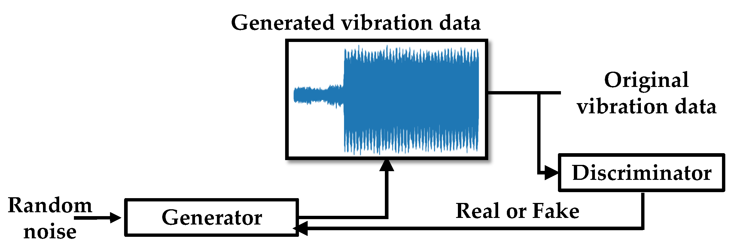
3.2. Use of GAN to Generate Realistic Vibration Data to Overcome Data Imbalance

This section introduces the GAN framework and training method of the target approach. Figure 4 displays the framework of the target GAN, which includes a generator and discriminator. The generator receives random noise and then generates a set of tool vibration data, whereas the discriminator receives the generated vibration data and the original vibration data and determines whether the generated vibration data are similar to the true data. The resulting determination is then provided to the generator as feedback. Based on the feedback, the generator then generates even more realistic tool vibration data for the discriminator to assess. The entire training process is repeated until the discriminator cannot determine whether the generated data are real or not.

The generator used in this study comprised three types of layers: an input layer, multiple upsampling layers, and multiple convolution layers. Below, we explain the input and the formulas of the neurons in each layer in the generator in detail. First, regarding the input data, suppose that the random data have $n$ items of data and $m$ features. Thus, the input is a $n\times m$ random number matrix, the elements of which are normally distributed random numbers between 0 and 1.

The input layer places the input data in the model. The input data of this layer are the output results, as follows:

$$O_i^{input}=x_i^{input},$$

(3)

where $O$ denotes the neuron output, $x$ represents the input data, and i is the ith input of the model.

The upsampling layers employ nearest-neighbor interpolation, copying existing data to augment the feature map so that the model can better learn the features of the data during training. With input n and sample size size, the formula of the upsampling layers is as follows:

$$O_i=x_{\lfloor i/size\rfloor }, i\in \left[0,n\times size\right), i\in N$$

(4)

where O_i represents the output of the $i$th neuron and $x_i$ denotes the $i$th input.

In convolution layers, each node has k kernels of size m. Thus, the formula of the convolutional layers is as follows:

$$O_i=act\left({{\displaystyle \sum }}_{k=0}^{k=m-1}{x}_{i+m-k}{w}_k+b_i\right),$$

(5)

where O_i represents the output of the $i$th neuron, $x_i$ denotes the $i$th original input, W is the filter, and act(•) is an activation function.

Table 2. The structure of the generator.

Layer	Type	Output Size	Kernel Size	Stride	Activation Function
Input	Input	$125\times 128$	-	-	-
U1	Upsampling	$250\times 128$	-	-	-
C2	Convolutional	$125\times 64$	3	2	LeakyReLU
U3	Upsampling	$250\times 64$	-	-	-
C4	Convolutional	$125\times 64$	3	2	LeakyReLU
U5	Upsampling	$250\times 64$	-	-	-
C6	Convolutional	$125\times 64$	3	2	LeakyReLU
U7	Upsampling	$250\times 64$	-	-	-
Output	Convolutional	$250\times 7$	-	-	tanh

shows the structure of the GAN generator as applied to the 2010 PHM dataset. The random numbers we input initially formed a 125 $\times$ 128 matrix. Then, aside from the input layer, the model itself also included four sets of upsampling and convolution layers. Note that the number of sets was decided via trial and error. Due to the high degree of detail that we desired from the produced signals, we set the kernel size and stride at 3 and 2, respectively. Finally, for the activation function, we used LeakyReLU in the first three convolutional layers to ensure that the features in the inputs could be fully displayed without falling into the dead zone. Due to the output signal values, we adopted tanh for the last convolutional layer to obtain better results. Finally, because the original 2010 PHM dataset contained seven dimensions, we set the number of dimensions in the generator output data to seven.

The discriminator used in this study employs a one-dimensional CNN, the input of which is real tool vibration data and the tool vibration data generated by the generator and the output is the degree of similarity between the two. The architecture of this CNN includes four types of layers: an input layer, multiple convolution layers, multiple batch normalization layers, and an output layer. The convolution layer and the batch normalization layer are used alternately.

The mathematical formulas of the input layer, convolution layers, and output layer are identical to those in the generator. The batch normalization layers help mitigate gradient vanishing and accelerate neural convergence, as follows:

$$O_i=\frac{x_i-\overline{x}}{\sqrt{Var\left(x_i\right)}}+\beta ,$$

(6)

where $O$ and $x$ denote the output and input, respectively, $i$ represents the ith neuron, and $\gamma$ and $\beta$ represent the scale and shift.

Once the generator and discriminator have been established, we used a backpropagation algorithm to train the two networks. The aim is to minimize generator loss, which means that the data generated by the generator are as close as possible to the ground truth, making it difficult for the discriminator to distinguish real data from generated data. The formula for generator loss is as follows:

$$GeneratorLoss=\frac{1}{N}{\displaystyle \sum }_{i=1}^N\log \left(1-D\left(G\left(R^i\right)\right)\right),$$

(7)

where R is a vector of random numbers, D and G represent the discriminator and generator, respectively, and N denotes the training data. With regard to the discriminator, the aim is to minimize discriminator loss, which means that the discriminator has the ability to distinguish real data from generated data. The formula for discriminator loss is as follows:

$$Discriminator=-\frac{1}{N}{{\displaystyle \sum }}_{i=1}^N\log D\left(X^i\right)-\frac{1}{N}{{\displaystyle \sum }}_{i=1}^N\log \left(1-D\left({\widehat{X}}^i\right)\right),$$

(8)

where X denotes the original data, $\widehat{X}$ represents the generator, D is the discriminator, and N denotes the training data.

Table 3. The structure of the discriminator.

Layer	Type	Output Size	Kernel Size	Stride	Activation Function
Input	Input	$250\times 7$	-	-	-
C1	Convolutional	$125\times 128$	3	2	LeakyReLU
C2	Convolutional	$63\times 128$	3	2	LeakyReLU
BN3	Batch normalization	$63\times 128$	-	-	-
C4	Convolutional	$63\times 64$	3	2	LeakyReLU
BN5	Batch normalization	$63\times 64$	-	-	-
C6	Convolutional	$63\times 64$	3	1	LeakyReLU
BN7	Batch normalization	$63\times 64$	-	-	-
Output	Fully connected	1	-	-	-

presents the structure of the GAN discriminator as applied to the 2010 PHM dataset. The realistic data generated by the generator and the real data were both input to the model. After the input layer, we used a convolutional layer to perform dimension reduction. We then used three sets of convolutional layers and batch normalization layers to check the generated data. The number of sets was also decided via trial and error. As for the kernel size and stride parameters, we adopted settings similar to those of the generator, setting them as 3 and from 1 to 2, respectively. Finally, for the activation function, the objective of the discriminator was to inspect whether the data features are reasonable. We therefore used LeakyReLU for all convolutional layers to ensure that the features in the inputs could be fully displayed without falling in the dead zone. Finally, we used a fully connected layer to gauge whether the output was realistic.

3.3. Feature Selection

This section introduces three methods that we used to extract the features of the vibration signals. The first method is time series feature extraction, in which changes in the amplitudes of tool cutting in the same time interval are analyzed. The second method is fast Fourier transform (FFT), in which the relationship between amplitude and frequency during tool cutting is observed and analyzed. The last method is continuous wavelet transform, in which changes in the amplitudes in time and frequency during tool cutting are observed and analyzed.

3.3.1. Time Series Feature Extraction

To extract the important features of the time series, researchers have used overlapping windows of a fixed size to segment time series into equal lengths and then extracted various feature statistics (including maximum, minimum, mean, sum, average absolute deviation, root mean square error, and standard deviation) from each segmented window [49]. In this study, we used this approach to extract the statistical features of the vibration data in all seven domains. Below, we introduce the formulas for each feature, assuming that the original dataset can be expressed as X $=\left[x_1,x_2,x_3,\dots ,x_n\right]$ and data X(t) in the window at time point t can be written as X(t)=[x_t, x_t+1, …, x_t+w], where w is the length of the window:

• $F_{Max}\left(t\right)$ is the maximum value in $X\left(t\right)$;
• $F_{Min}\left(t\right)$ is the minimum value in $X\left(t\right)$;
• $F_{avg}\left(t\right)$ is the mean of all values in $X\left(t\right)$;
• $F_{sum}\left(t\right)$ is the sum of all values in $X\left(t\right)$;
• $F_{mad}\left(t\right)$ is the degree of dispersion among all values in $X\left(t\right)$:

  $$MAD=\frac{1}{\left|t\right|}{{\displaystyle \sum }}_{i=1}^{\left|t\right|}\left|x_i-m\right|,$$

  (9)
• $F_{RMSE}\left(t\right)$ is the root mean square error of all values in X(t):

  $$RMSE=\sqrt{\frac{1}{\left|t\right|}{{\displaystyle \sum }}_{i=1}^{\left|t\right|}{x}_i^2},$$

  (10)
• $F_{std}\left(t\right)$ is the standard deviation of all of the values in X(t):

  $$STD=\sqrt{\frac{{{\displaystyle \sum }}_{i=1}^n{\left(x_i-\overline{x}\right)}^2}{n-1} },$$

  (11)

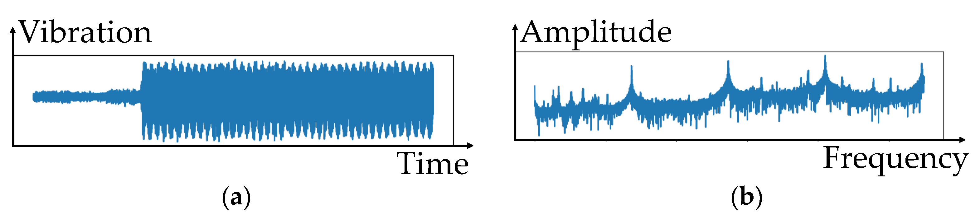
3.3.2. Fast Fourier Transform (FFT)

Tool vibration data are continuous, and many researchers have analyzed such data using FFT [50,51,52,53]. FFT is an accelerated form of the discrete Fourier transform which converts time-domain data into the frequency domain for the convenience of users. Its formula is as follows:

$$x\left(e^{j{\widehat{\omega }}_{\mathrm{k}}}\right)={{\displaystyle \sum }}_{n=0}^{L-1}x\left[n\right]e^{j{\widehat{\omega }}_{\mathrm{k}}n},$$

(12)

where x($e^{j{\widehat{\omega }}_k})$ is a continuous function of frequency, ${\widehat{\omega }}_k$ is a certain frequency sample equaling $\frac{2\pi k}{N}$, and L denotes the length of $x\left[n\right]$. This formula analyzes the components of the signal (i.e., the total proportions of various frequencies), as shown in Figure 5. Using this technique, the model can subsequently learn the features of the tool-wear data in the frequency domain.

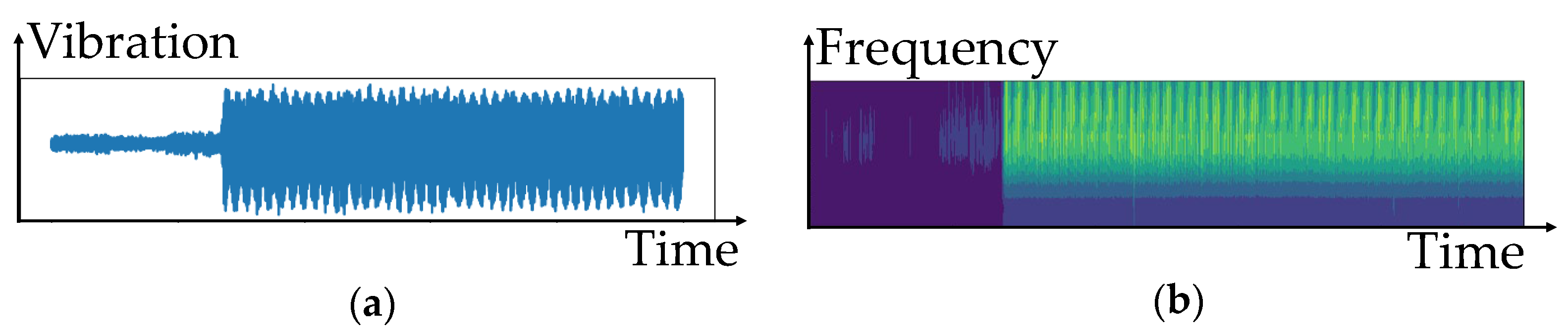
3.3.3. Continuous Wavelet Transform

The continuous wavelet transform technique was first proposed by Grossman et al. [54]. It uses a continuous function to process continuous time data, thereby obtaining a wavelet coefficient to analyze changes in frequency at different times and extensions. Ultimately, the goal of converting the time series data into time–frequency domain data is achieved. Due to space restrictions and the maturity of this technique, we will not go into the details here. Figure 6 displays an example of transformed tool-wear vibration data. This figure clearly shows that the two sections with completely different vibration signals remain different following conversion into a time–frequency graph.

3.4. CNN

We employed a CNN to model the different features. The input of the model can be features extracted using any of the methods discussed in the previous section. The output of the model is the classification of tool-wear status, which can be the rapid initial wear, uniform wear, or failure wear. The framework has one input layer, n convolutional layers, n max pooling layers, and m fully connected layers. The convolutional and max pooling layers are alternated. As the CNN is widely applied, we present only a brief introduction to its framework.

Regarding the input data, suppose that the original data contain n items of data and m features. Thus, the original data will form an $n\times m$ matrix. Applying the feature selection methods to the data then produces h important feature values, from which an $n\times m\times h$ input data matrix can be obtained.

The input layer places the input data in the model. The input data of this layer are the output results, as follows:

$$O_i^{input}=x_i^{input},$$

(13)

where O denotes the neuron output, x represents the input data, and i is the ith input of the model.

The purpose of the convolutional layers is to extract each local feature by sliding a filter along the series data. Each node of the neurons in the designed convolutional layers has k kernels of size m. Ultimately, we can write the formula of the neurons as follows:

$$O_i=act\left({{\displaystyle \sum }}_{k=0}^{k=m-1}{x}_{i+m-k}{w}_k+b_i\right),$$

(14)

where $O_i$ represents the output of the ith neuron, $x_i$ denotes the ith original input, w is the filter, $act(•)$ is an activation function (for which we used Relu), and $b_i$ denotes the bias value of the ith neuron.

Then there are the max pooling layers. Suppose that the input dimensions are ($L_i$,$D_i$) and the pooling size and stride of the layers are p and s, respectively. Then, the formula of this layer can be written as follows:

$$L_y=\frac{L_i-p_i}{s}+1,$$

(15)

$$D_y=D_i,$$

(16)

and the final output is ($L_y,D_y$).

The purpose of the fully connected layers is to integrate the outputs of the neurons of the previous layer and then output the classification results. The formula of each neuron is as follows:

$$O_j=act\left(x_j\times w_{ij}\right)+b_j,$$

(17)

where $O_j$ represents the output of the jth neuron, $x_j$ is the input of the jth neuron, $w_{ij}$ denotes the weight of the connection with the previous layer, $b_j$ is the bias value of the jth neuron, and $act(\bullet )$ is an activation function. If the fully connected layer is used to output the classification results, then we use the Softmax activation function; if not, then the Relu activation function is used. Finally, the entire model is trained using backpropagation.

Table 4. The structure of the convolutional neural network.

Layer	Type	Output Size	Kernel Size	Stride	Activation Function
Input	Input	$m\times h$	-	-	-
C1	Convolutional	$h\times 2^{{\log }_2\left[m\ast 2\right]+1}$	3	1	Relu
P2	Max pooling	$\left(h/2\right)\times 2^{{\log }_2\left[m\ast 2\right]+1}$	-	-	-
C3	Convolutional	$\left(h/2\right)\times 2^{{\log }_2\left[m\ast 2\right]+2}$	3	1	Relu
P4	Max pooling	$\left(h/4\right)\times 2^{{\log }_2\left[m\ast 2\right]+2}$	-	-	-
C5	Convolutional	$\left(h/4\right)\times 2^{{\log }_2\left[m\ast 2\right]+3}$	3	1	Relu
P6	Max pooling	$\left(h/8\right)\times 2^{{\log }_2\left[m\ast 2\right]+3}$	-	-	-
C7	Convolutional	$\left(h/8\right)\times 2^{{\log }_2\left[m\ast 2\right]+3}$	3	1	Relu
P8	Max pooling	$\left(h/16\right)\times 2^{{\log }_2\left[m\ast 2\right]+3}$	-	-	-
F9	Fully connected	512	-	-	Relu
Output	Fully connected	3	-	-	softmax

exhibits the structure of the CNN as applied to the 2010 PHM dataset. In this table, h denotes the number of important features extracted and m is the original number of features. The target CNN contained four sets of convolutional layers and max pooling layers, which would gradually flatten out the important features and thereby enable the extraction of the key factors for classification. We then set the kernel size and stride of the convolutional layers as 3 and 1, respectively, to ensure a full examination of the data. As with most CNN frameworks, we used the Relu activation function in the convolutional layers. Finally, we used two fully connected layers to estimate the output results. As the last layer outputs the classification results, we adopted the Softmax activation function.

3.5. Use of SNN to Achieve Ensemble Learning

This section introduces the use of an SNN to achieve ensemble learning. First, regarding the input data, suppose that we use a total of h methods to extract the features and that each model has n classification results for tool-wear status. Thus, the input data can be expressed using an $h\times n$ matrix. Then, the input layer places the input data in the model. The input data of this layer are the output results, as follows:

$$O_i^{input}=x_i^{input},$$

(18)

where O denotes the neuron output, x represents the input data, and i is the ith input of the model.

The hidden layer of the SNN comprises multiple fully connected layers, the number of which is determined by the number of previous neurons. Suppose that the output of the previous neuron is $\alpha$. The fully connected layer has a total of ${\log }_2\alpha$ layers. The neurons on each layer integrate the outputs of the neurons in the previous layer, and they are all fully connected. Thus, the formula is as follows:

$$O_j=\left(x_j\times w_{ij}\right)+b_j,$$

(19)

where $O_j$ represents the output of the jth neuron, $x_j$ is the input of the jth neuron, $w_{ij}$ denotes the weight of the connection with the previous layer, and $b_j$ is the bias value of the jth neuron.

The objective of the final output layer is to combine the outputs of all the neurons of the previous layer, input them to the activation function, and then output the results. The formula is as follows:

$$O_j=act\left(x_j\times w_{ij}\right)+b_j,$$

(20)

where $O_j$ represents the output of the jth neuron, $x_j$ is the input of the jth neuron, $w_{ij}$ denotes the weight of the connection with the previous layer, and $b_j$ is the bias value of the jth neuron. The target problem is a classification problem, so we use the Softmax activation function for $act(•)$.

After modeling, the weights are updated using backpropagation, and the model is trained repeatedly until maximum accuracy is obtained.

4. Experiments

Experiments were conducted to demonstrate the efficiency of the proposed methods. All models and experiments were completed using Python on an Intel Core i7-9700KF CPU at 3.6 GHz with 16 GB member, Nvidia RTX 2080 ti 8 GB GPU, and the Windows 10 operating system.

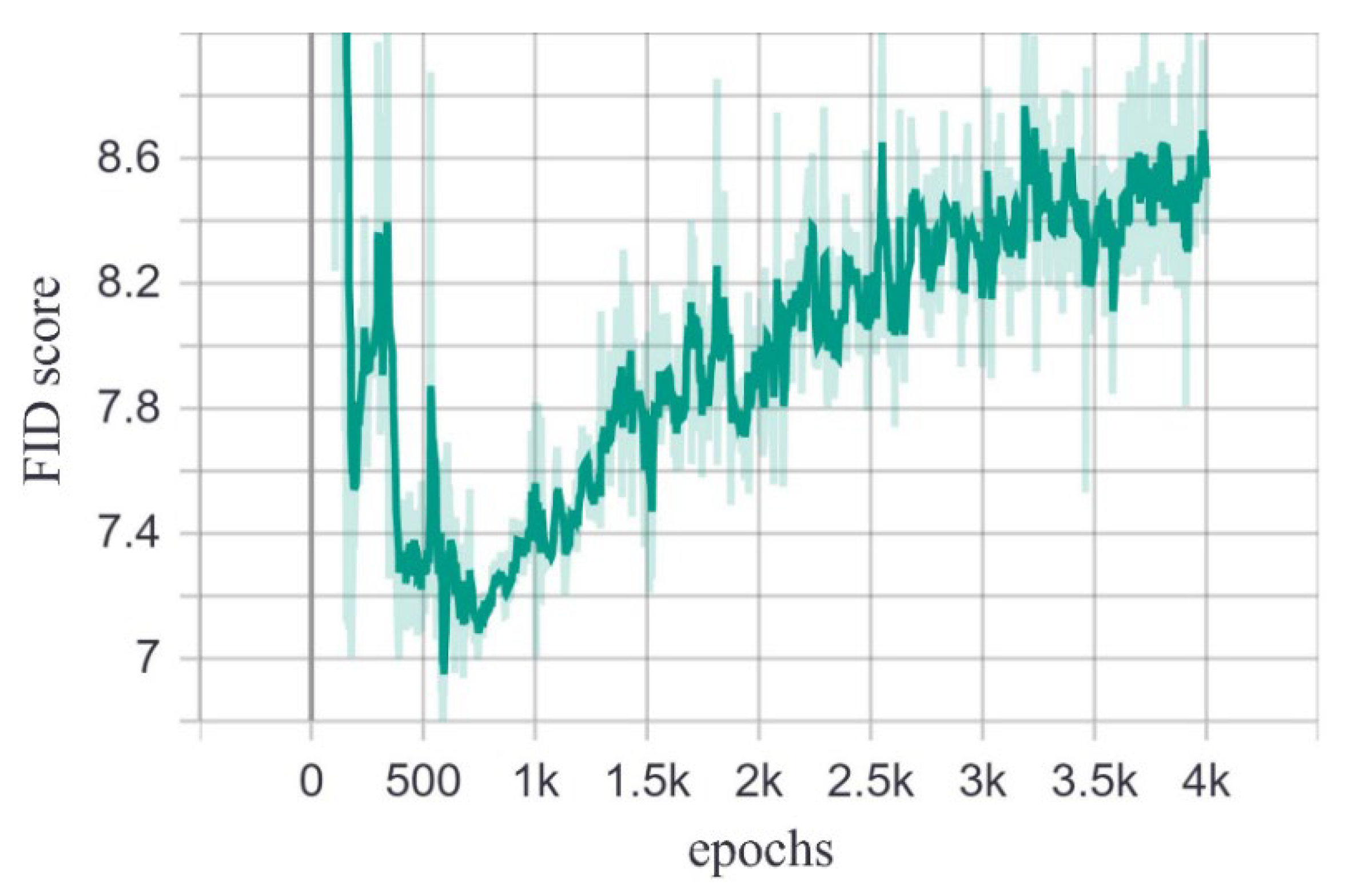
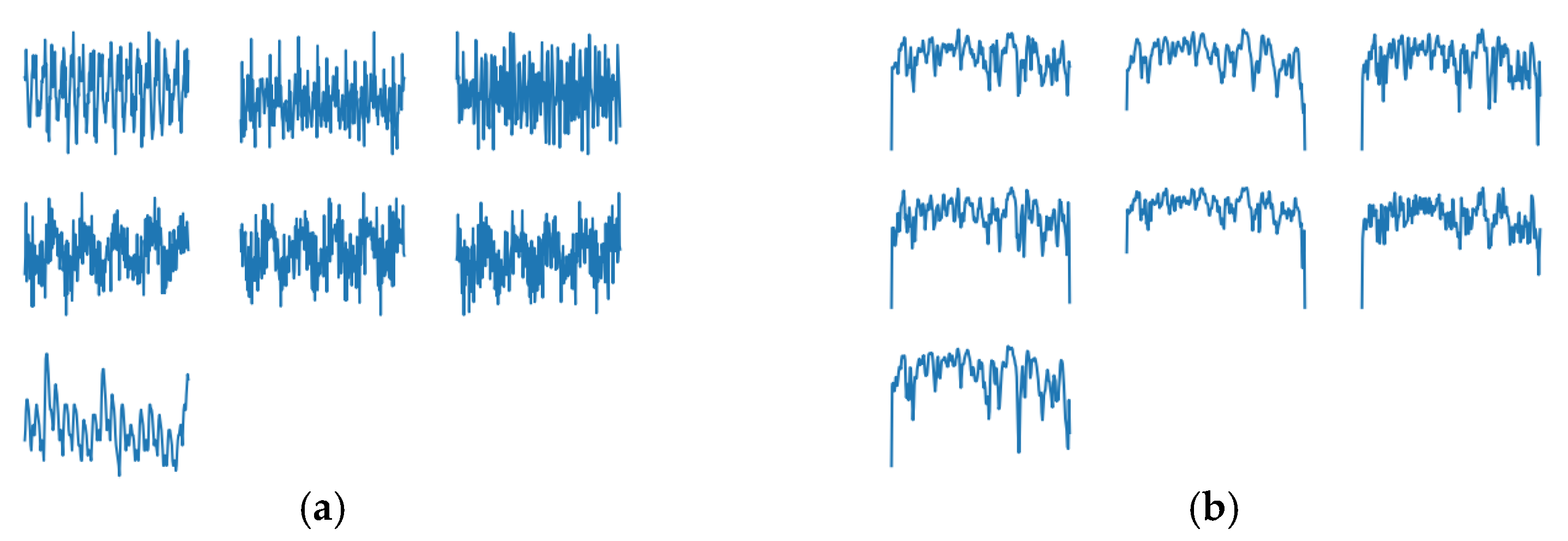
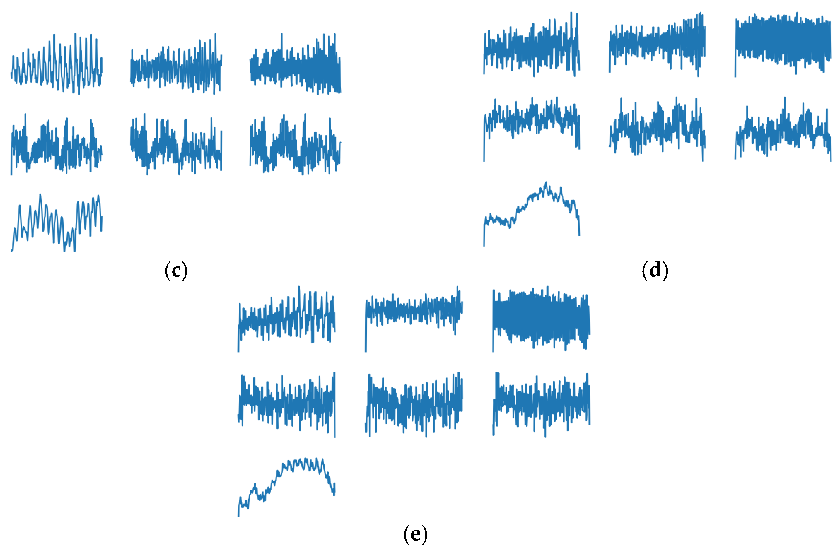
4.1. Results of Using GAN to Generate Data

This section introduces the parameter settings of the target GAN and the results of using realistic data to complete the original data. First, all training data were normalized using the tool ‘minmaxscaler’. We then used the popular tool “Adam” as the optimizer. Through trial and error, we determined that the optimal learning rate was 0.0002. We set the upper limit for epochs at 4000, which takes one day to complete in the selected environment and fits neatly within factory work schedules. For performance evaluation, we referred to Heusel et al. [55] in our use of the Frechet inception distance (FID) score to assess model similarity and the number of iterations to ensure that the distribution of the generated data resembled that of the original data. The FID score calculates the Gaussian distribution distance between the feature vectors of real images and generated images. A smaller value indicates that the Gaussian distribution of the generated image is closer to that of the real image. Figure 7 displays the FID scores during the training process. Observation shows that the FID score was smallest at the 800th epoch, meaning that this distribution was closest to real statuses. Figure 8 compares the generated data under different numbers of epochs. As can be seen, after 800 epochs, the data generated by the GAN model deviated from the original data (Figure 8a), whereas the data generated by the GAN model trained for 800 epochs were similar to the original data. This result corresponds with the FID score results. The results of Figure 7 and Figure 8 indicate that the GAN is subject to overfitting after 800 epochs. Hence, in the following experiments, we trained the model for 800 epochs.

After identifying the optimal parameter settings, we used the GAN to capture rapid initial wear and failure wear data, and the amounts of these two classifications of data were identical to those of uniform wear data. Ultimately, the proportions of original data and GAN-generated data were as shown in Figure 9.

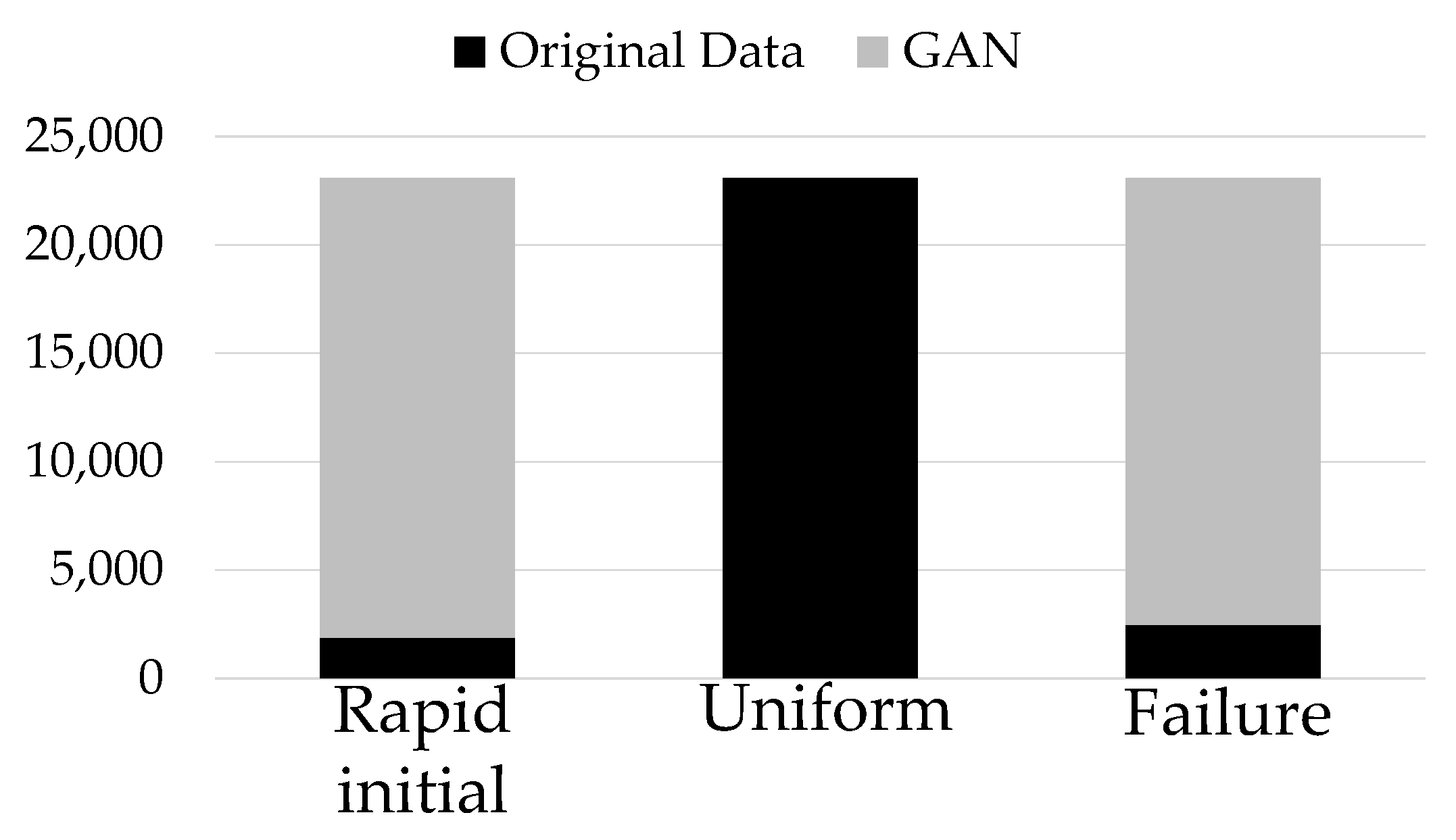
4.2. Validity of Using GAN-Generated Data to Overcome Imbalance in Tool-Wear Data

To verify the validity of using GAN-generated data to overcome data imbalance, we compared the proposed approach with four other methods: (1) directly using the original data without balancing; (2) using augmentation methods to balance the data [56,57]; (3) using SMOTE to balance the data [58,59,60]; and (4) using downsampling to balance the data [57,61,62]. We compared these five methods by using them to generate a new training set. For the first method, we copied all the original data into the training set. For the second and third methods, we employed the same approach as the proposed GAN method and generated large quantities of rapid initial wear and failure wear data so that the amounts of these two classifications of data equaled that of the uniform wear data. For the final fourth method, with the amount of rapid initial wear data as the benchmark, we randomly extracted the same amount of uniform wear and failure wear data to form the training set. Once the training sets were generated, we used the three feature selection methods (time series feature extraction, FFT, and continuous wavelet transform) to extract important features. The results of each method were used to train a CNN. We therefore trained a total of 15 models (5 methods of handling data imbalance × 3 feature selection methods). Finally, we input the 13,586 items of the original data into these 15 models and observed their prediction results. We used two indices to examine the quality of the prediction results: accuracy and recall. We specifically used recall rather than precision because manufacturers are generally more concerned with the identification of real tool-wear statuses rather than whether each of the predictions is correct.

Table 5. Comparison of the accuracy of all combinations of data balancing and feature extraction methods.

	Time Series Feature Extraction	FFT	Continuous Wavelet Transform
Original data	90.08%	88.13%	94.41%
Augmentation	83.40%	84.01%	93.51%
SMOTE	83.45%	82.88%	92.67%
Downsampling	86.09%	86.22%	95.05%
GAN	88.17%	85.85%	96.50%

compares the accuracy values of the 15 models. In this table, we first compared the prediction results of the method using the original data and those of the other methods. Surprisingly, among the methods using time series and FFT, those modeled using the original data had the highest accuracy. Furthermore, among the methods using the continuous wavelet transform, the one modeled using the original data had the third highest accuracy. We speculated that this was because the training data were identical to the test data, and naturally, this led to the highest accuracy. However, in practice, training data would never be identical to test data. Thus, in subsequent analyses, we merely used the prediction data of the methods modeled using the original data as high standards for the other methods (i.e., the prediction results that the models could achieve under the best circumstances). If we apply this standard to assess the prediction performance of the proposed GAN approach, its results come close. This serves as preliminary confirmation of the reasonableness of the proposed approach.

Then, we compared the prediction performance of the GAN approach with that of the other three data-balancing methods. We found that, regardless of the feature extraction method, the GAN approach provided the most accurate prediction results. This demonstrates that the GAN approach is indeed superior to existing methods in overcoming data imbalance. However, we must mention that the prediction accuracy of the GAN approach paired with FFT was slightly lower than that of the downsampling method. We speculate that this is due to sampling errors in downsampling and the fact that the sample data coincidentally had a distribution similar to that of the test data.

Table 6. Comparison of recall of all combinations of methods with different tool-wear classifications.

	Time Series Feature Extraction			FFT			Continuous Wavelet Transform
	Rapid Initial	Uniform	Failure	Rapid Initial	Uniform	Failure	Rapid Initial	Uniform	Failure
Number of data	124	9919	3543	124	9919	3543	124	9919	3543
Original data	98.39%	96.22%	72.88%	100.00%	84.50%	98.11%	0.00%	97.43%	89.53%
Augmentation	100.00%	86.95%	73.13%	100.00%	93.30%	57.69%	84.68%	93.93%	92.89%
SMOTE	100.00%	88.03%	70.31%	100.00%	85.35%	75.61%	83.87%	92.48%	93.76%
Downsampling	100.00%	87.68%	81.40%	100.00%	88.05%	80.86%	45.16%	96.85%	92.01%
GAN	97.58%	98.75%	58.51%	100.00%	98.40%	50.52%	64.52%	98.93%	91.08%

compares the recall results of the 15 models with different tool-wear classifications. For the sake of convenience, we presented the amounts of test data for each type of classification. As can be seen, for uniform wear, the recall of the GAN approach was close to 99% and far higher than that of any other method regardless of the feature extraction method. However, for rapid initial wear and failure wear, the recall values were slightly or far lower than those of the other methods. At first glance, these results show that the GAN approach offers no advantages; however, in practice, manufacturers are most interested in the identification of uniform wear status (as stated in the example in Section 1). Rapid initial wear is usually not of concern because it is rare. With regard to failure wear, we can see from Table 6 that the amount of failure wear data is about one-third that of uniform wear, but in practice, tools are generally replaced as soon as failure wear occurs. Thus, there is rarely such a large quantity of failure wear data, which means that manufacturers have little interest in accuracy rates for this classification. Based on the above arguments, we can see that the efficacy of the proposed GAN approach remains valid.

4.3. Verification of Necessity of Multiple Feature Extraction Methods for Tool Wear

Most existing studies used a single feature extraction method to predict tool wear. However, we believe that this approach is flawed and therefore used three feature extraction methods for tool-wear prediction. We then combined the prediction results of these methods to derive our final prediction results. We use

Table 7. Comparison of recall of different feature extraction methods for different tool-wear statuses.

	Rapid Initial Wear (Recall)	Uniform Wear (Recall)	Failure Wear (Recall)
Time series feature extraction	97.58%	98.75%	58.51%
FFT	100.00%	98.40%	50.52%
Continuous wavelet transform	64.52%	98.93%	91.08%
Ensemble	98%	99%	88%

to verify this approach. The table compares the recall results of the three feature extraction methods with the ensemble model.

We first observed the results of the three individual feature extraction methods, which clearly show that the prediction results of time series and FFT were better with regard to rapid initial wear and uniform wear but were poorer with regard to failure wear. We speculate that because these two methods only consider time or frequency information, the features of which do not differ significantly at the junction in uniform wear and failure wear, they could not differentiate between failure wear and uniform wear data. Then, we found that the continuous wavelet transform approach produced better prediction results for uniform wear and failure wear but poor prediction results for rapid initial wear. We believe that this is because the wavelet transform approach extracts the time and frequency features from the data at the same time, which benefits the identification of uniform wear and failure wear data at the junction. However, this also provided too much information and made it difficult to differentiate between the relatively simple rapid initial wear and uniform wear.

Then, comparing the results of the ensemble model with those of the three feature extraction methods, we found that the ensemble model could achieve relatively good accuracy for all three tool-wear statuses. Compared to the three feature extraction methods, which could only obtain superior results for two tool-wear statuses, the results of the ensemble model were significantly better. This demonstrates the validity of using the ensemble approach to integrate different feature extraction methods.

5. Conclusions and Directions for Future Research

Traditionally, manufacturers have relied on experience to determine when a tool should be replaced. While many researchers have developed algorithms to automate this process using CNC machine operating data, most existing studies focus on model development and neglect two fundamental issues in machine learning: data imbalance and feature extraction. In view of this, we applied two approaches for improvement: (1) using a GAN to generate realistic CNC machine vibration data to overcome data imbalance and (2) extracting features in the time, frequency, and time–frequency domains simultaneously and integrating these in an ensemble model. The experimental results demonstrate the validity of the proposed approaches.

In future work, we plan to modify the proposed GAN into a conditional GAN to consider other relevant factors that influence tool wear, such as spindle speed or feed rate, to produce more realistic data.

References

1. Hu, Y.; Miao, X.; Si, Y.; Pan, E.; Zio, E. Prognostics and health management: A review from the perspectives of design, development and decision. Reliab. Eng. Syst. Saf. 2022, 217, 108063. [Google Scholar] [CrossRef]
2. Zio, E. Prognostics and Health Management (PHM): Where are we and where do we (need to) go in theory and practice. Reliab. Eng. Syst. Saf. 2022, 218, 108119. [Google Scholar] [CrossRef]
3. Vrignat, P.; Kratz, F.; Avila, M. Sustainable manufacturing, maintenance policies, prognostics and health management: A literature review. Reliab. Eng. Syst. Saf. 2022, 218, 108140. [Google Scholar] [CrossRef]
4. Sun, C.; Wang, P.; Yan, R.Q.; Gao, R.X.; Chen, X.F. Machine health monitoring based on locally linear embedding with kernel sparse representation for neighborhood optimization. Mech. Syst. Signal Processing 2019, 114, 25–34. [Google Scholar] [CrossRef]
5. Sun, C.; Ma, M.; Zhao, Z.; Tian, S.; Yan, R.; Chen, X. Deep transfer learning based on sparse auto-encoder for remaining useful life prediction on tool in manufacturing. IEEE Trans. Ind. Inform. 2018, 15, 2416–2425. [Google Scholar] [CrossRef]
6. Chen, B.; Chen, X.; Li, B.; He, Z.; Cao, H.; Cai, G. Reliability estimation for cutting tools based on logistic regression model using vibration signals. Mech. Syst. Signal Processing 2011, 25, 2526–2537. [Google Scholar] [CrossRef]
7. Kong, D.; Chen, Y.; Li, N. Gaussian process regression for tool wear prediction. Mech. Syst. Signal Processing 2018, 104, 556–574. [Google Scholar] [CrossRef]
8. Benkedjouh, T.; Medjaher, K.; Zerhouni, N.; Rechak, S. Health assessment and life prediction of cutting tools based on support vector regression. J. Intell. Manuf. 2015, 26, 213–223. [Google Scholar] [CrossRef] [Green Version]
9. Cai, G.; Chen, X.; Chen, B.L.B.; He, Z. Operation reliability assessment for cutting tools by applying a proportional covariate model to condition monitoring information. Sensors 2012, 12, 12964–12987. [Google Scholar] [CrossRef] [PubMed] [Green Version]
10. Zhu, K.; Liu, T. Online Tool Wear Monitoring via Hidden Semi-Markov Model with Dependent Durations. IEEE Trans. Ind. Inform. 2018, 14, 69–78. [Google Scholar] [CrossRef]
11. Yu, J.; Liang, S.; Tang, D.; Liu, H. A weighted hidden Markov model approach for continuous-state tool wear monitoring and tool life prediction. Int. J. Adv. Manuf. Technol. 2017, 91, 201–211. [Google Scholar] [CrossRef]
12. Kurek, J.; Wieczorek, G.; Kruk, B.S.M.; Jegorowa, A.; Osowski, S. Transfer learning in recognition of drill wear using convolutional neural network. In Proceedings of the 2017 18th International Conference on Computational Problems of Electrical Engineering (CPEE), Kutna Hora, Czech Republic, 11–13 September 2017. [Google Scholar]
13. Rohan, A. A Holistic Fault Detection and Diagnosis System in Imbalanced, Scarce, Multi-Domain (ISMD) Data Setting for Component-Level Prognostics and Health Management (PHM). arXiv 2022, arXiv:2204.02969. [Google Scholar] [CrossRef]
14. Zhang, J.; Wang, P.; Yan, R.; Gao, R. Deep Learning for Improved System Remaining Life Prediction. Procedia CIRP 2018, 72, 1033–1038. [Google Scholar] [CrossRef]
15. Cao, P.; Zhang, S.; Tan, J. Preprocessing-Free Gear Fault Diagnosis Using Small Datasets with Deep Convolutional Neural Network-Based Transfer Learning. IEEE Access 2018, 6, 26241–26253. [Google Scholar] [CrossRef]
16. Chiu, S.M.; Chen, Y.C.; Kuo, C.J.; Hung, L.C.; Hung, M.H.; Chen, C.C.; Lee, C. Development of Lightweight RBF-DRNN and Automated Framework for CNC Tool-Wear Prediction. IEEE Trans. Instrum. Meas. 2022, 71, 2506711. [Google Scholar] [CrossRef]
17. Carino, J.A.; Delgado-Prieto, M.; Iglesias, J.A.; Sanchis, A.; Zurita, D.; Millan, M.; Redondo, J.A.O.; Romero-Troncoso, R. Fault Detection and Identification Methodology under an Incremental Learning Framework Applied to Industrial Machinery. IEEE Access 2018, 6, 49755–49766. [Google Scholar] [CrossRef]
18. Brito, L.C.; da Silva, M.B.; Duarte, M.A.V. Identification of cutting tool wear condition in turning using self-organizing map trained with imbalanced data. J. Intell. Manuf. 2021, 32, 127–140. [Google Scholar] [CrossRef]
19. Miao, H.; Zhao, Z.; Sun, C.; Li, B.; Yan, R. A U-Net-Based Approach for Tool Wear Area Detection and Identification. IEEE Trans. Instrum. Meas. 2021, 70, 5004110. [Google Scholar] [CrossRef]
20. Rohan, A.; Raouf, I.; Kim, H.S. Rotate Vector (RV) Reducer Fault Detection and Diagnosis System: Towards Component Level Prognostics and Health Management (PHM). Sensors 2020, 20, 6845. [Google Scholar] [CrossRef]
21. Goodfellow, I.; Pouget-Abadie, J.; Mirza, M.; Xu, B.; Warde-Farley, D.; Ozair, S.; Aaron, C.; Bengio, Y. Generative adversarial nets. Adv. Neural Inf. Processing Syst. 2014, 27, 2672–2680. [Google Scholar]
22. Karras, T.; Aila, T.; Laine, S.; Lehtinen, J. Progressive Growing of GANs for Improved Quality, Stability, and Variation. arXiv 2017, arXiv:1710.10196. [Google Scholar]
23. Yadav, N.K.; Singh, S.K.; Dubey, S.R. CSA-GAN: Cyclic synthesized attention guided generative adversarial network for face synthesis. Appl. Intell. 2022. [Google Scholar] [CrossRef]
24. Shi, Y.; Aggarwal, D.; Jain, A.K. Lifting 2D StyleGAN for 3D-Aware Face Generation. In Proceedings of the IEEE/CVF Conference on Computer Vision and Pattern Recognition (CVPR), Nashville, TN, USA, 20–25 June 2021; pp. 6258–6266. [Google Scholar]
25. Fang, Z.; Liu, Z.; Liu, T.; Hung, C.C.; Xiao, J.; Feng, G. Facial expression GAN for voice-driven face generation. Vis. Comput. 2022, 38, 1151–1164. [Google Scholar] [CrossRef]
26. Chen, Y.; Zhang, H.; Liu, L.; Chen, X.; Zhang, Q.; Yang, K.; Xia, R.; Xie, J. Research on image Inpainting algorithm of improved GAN based on two-discriminations networks. Appl. Intell. 2021, 51, 3460–3474. [Google Scholar] [CrossRef]
27. Wei, D.; Huang, K.; Ma, L.; Hua, J.; Lai, B.; Shen, H. OAW-GAN: Occlusion-aware warping GAN for unified human video synthesis. Appl. Intell. 2022, 1–18. [Google Scholar] [CrossRef]
28. Tagawa, Y.; Maskeliūnas, R.; Damaševičius, R. Acoustic Anomaly Detection of Mechanical Failures in Noisy Real-Life Factory Environments. Electronics 2021, 10, 2329. [Google Scholar] [CrossRef]
29. Zhang, F.; Ma, Y.; Yuan, G.; Zhang, H.; Ren, J. Multiview image generation for vehicle reidentification. Appl. Intell. 2021, 51, 5665–5682. [Google Scholar] [CrossRef]
30. Gan, Y.S.; Liong, S.-T.; Wang, S.-Y.; Cheng, C.T. An improved automatic defect identification system on natural leather via generative adversarial network. Int. J. Comput. Integr. Manuf. 2022, 1–17. [Google Scholar] [CrossRef]
31. Gu, J.; Qi, Y.; Zhao, Z.; Su, W.; Su, L.; Li, K.; Pecht, M. Fault diagnosis of rolling bearings based on generative adversarial network and convolutional denoising auto-encoder. J. Adv. Manuf. Sci. Technol. 2022, 2, 2022009. [Google Scholar] [CrossRef]
32. Wang, M.; Zhou, J.; Gao, J.; Li, Z.; Li, E. Milling Tool Wear Prediction Method Based on Deep Learning under Variable Working Conditions. IEEE Access 2020, 8, 140726–140735. [Google Scholar] [CrossRef]
33. ISO 3685:1993; Tool-Life Testing with Single-point Turning Tools. International Organization for Standardization: Geneva, Switzerland, 1993.
34. Ertürk, Ş.; Kayabaşi, O. Investigation of the Cutting Performance of Cutting Tools Coated with the Thermo-Reactive Diffusion (TRD) Technique. IEEE Access 2019, 7, 106824–106838. [Google Scholar] [CrossRef]
35. Bhuiyan, M.S.H.; Choudhury, I.A.; Dahari, M.; Nukman, Y. Application of acoustic emission sensor to investigate the frequency of tool wear and plastic deformation in tool condition monitoring. Measurement 2016, 92, 208–217. [Google Scholar] [CrossRef]
36. Dolinšek, S.; Kopač, J. Acoustic emission signals for tool wear identification. Wear 1999, 225, 295–303. [Google Scholar] [CrossRef]
37. Bhuiyan, M.S.H.; Choudhury, I.A.; Nukma, Y.n. An innovative approach to monitor the chip formation effect on tool state using acoustic emission in turning. Int. J. Mach. Tools Manuf. 2012, 58, 19–28. [Google Scholar]
38. Li, Z.; Liu, R.; Wu, D. Data-driven smart manufacturing: Tool wear monitoring with audio signals and machine learning. J. Manuf. Processes 2019, 48, 66–76. [Google Scholar] [CrossRef]
39. Gomes, M.C.; Brito, L.C.; da Silva, M.B.; Duarte, M.A.V. Tool wear monitoring in micromilling using Support Vector Machine with vibration and sound sensors. Precis. Eng. 2021, 67, 137–151. [Google Scholar] [CrossRef]
40. Mohanraj, T.; Yerchuru, J.; Krishnan, H.; Aravind, R.S.N.; Yameni, R. Development of tool condition monitoring system in end milling process using wavelet features and Hoelder’s exponent with machine learning algorithms. Measurement 2021, 173, 108671. [Google Scholar] [CrossRef]
41. Jalali, S.K.; Ghandi, H.; Motamedi, M. Intelligent condition monitoring of ball bearings faults by combination of genetic algorithm and support vector machines. J. Nondestruct. Eval. 2020, 39, 25. [Google Scholar] [CrossRef]
42. Corne, R.; Nath, C.; el Mansori, M.; Kurfess, T. Study of spindle power data with neural network for predicting real-time tool wear/breakage during inconel drilling. J. Manuf. Syst. 2017, 43, 287–295. [Google Scholar] [CrossRef]
43. Hesser, D.F.; Markert, B. Tool wear monitoring of a retrofitted CNC milling machine using artificial neural networks. Manuf. Lett. 2019, 19, 1–4. [Google Scholar] [CrossRef]
44. Zhao, R.; Yan, R.; Wang, J.; Mao, K. Learning to monitor machine health with convolutional bi-directional LSTM networks. Sensors 2017, 17, 273. [Google Scholar] [CrossRef] [PubMed]
45. Cheng, C.; Li, J.; Liu, Y.; Nie, M.; Wang, W. Deep convolutional neural network-based in-process tool condition monitoring in abrasive belt grinding. Comput. Ind. 2019, 106, 1–13. [Google Scholar] [CrossRef]
46. Zhao, R.; Wang, D.; Yan, R.; Mao, K.; Shen, F.; Wang, J. Machine health monitoring using local feature-based gated recurrent unit networks. IEEE Trans. Ind. Electron. 2017, 65, 1539–1548. [Google Scholar] [CrossRef]
47. 2010 PHM Society Conference Data Challenge. Available online: https://www.phmsociety.org/competition/phm/10 (accessed on 1 June 2022).
48. Chen, Y.C.; Li, D.C. Selection of key features for PM2.5 prediction using a wavelet model and RBF-LSTM. Appl. Intell. 2021, 51, 2534–2555. [Google Scholar] [CrossRef]
49. Kuo, C.J.; Ting, K.C.; Chen, Y.C.; Yang, D.L.; Chen, H.M. Automatic machine status prediction in the era of industry 4.0: Case study of machines in a spring factory. J. Syst. Archit. 2017, 81, 44–53. [Google Scholar] [CrossRef]
50. Duerden, A.; Marshall, F.E.; Moon, N.; Swanson, C.; Donnell, K.; Grubbs, G.S., II. A chirped pulse Fourier transform microwave spectrometer with multi-antenna detection. J. Mol. Spectrosc. 2021, 376, 111396. [Google Scholar] [CrossRef]
51. Xu, W.; Xu, K.J.; Yu, X.L.; Huang, Y.; Wu, W.K. Signal processing method of bubble detection in sodium flow based on inverse Fourier transform to calculate energy ratio. Nucl. Eng. Technol. 2021, 53, 3122–3125. [Google Scholar] [CrossRef]
52. Jalayer, M.; Orsenigo, C.; Vercellis, C. Fault detection and diagnosis for rotating machinery: A model based on convolutional LSTM, Fast Fourier and continuous wavelet transforms. Comput. Ind. 2021, 125, 103378. [Google Scholar] [CrossRef]
53. Koga, K. Signal processing approach to mesh refinement in simulations of axisymmetric droplet dynamics. J. Comput. Appl. Math. 2021, 383, 113131. [Google Scholar] [CrossRef]
54. Grossmann, A.; Kronland-Martinet, R.; Morlet, J. Reading and Understanding Continuous Wavelet Transforms. In Wavelets. Inverse Problems and Theoretical Imaging; Combes, J.M., Grossmann, A., Tchamitchian, P., Eds.; Springer: Berlin/Heidelberg, Germany, 1989. [Google Scholar]
55. Heusel, M.; Ramsauer, H.; Unterthiner, T.; Nessler, B.; Hochreiter, S. GANs trained by a two time-scale update rule converge to a local nash equilibrium. In Proceedings of the International Conference on Neural Information Processing Systems (NIPS’17), Long Beach, CA, USA, 4–9 December 2017; pp. 6629–6640. [Google Scholar]
56. Shorten, C.; Khoshgoftaar, T.M. A survey on image data augmentation for deep learning. J. Big Data 2019, 6, 1–48. [Google Scholar] [CrossRef]
57. Koziarski, M.; Kwolek, B.; Cyganek, B. Convolutional neural network-based classification of histopathological images affected by data imbalance. In Proceedings of the Video Analytics. Face and Facial Expression Recognition, 3rd International Workshop, FFER 2018, and 2nd International Workshop, DLPR 2018, Beijing, China, 20 August 2018; pp. 1–11. [Google Scholar]
58. Bustillo, A.; Rodríguez, J.J. Online breakage detection of multitooth tools using classifier ensembles for imbalanced data. Int. J. Syst. Sci. 2014, 45, 2590–2602. [Google Scholar] [CrossRef]
59. Mathew, J.; Pang, C.K.; Luo, M.; Leong, W.H. Classification of imbalanced data by oversampling in kernel space of support vector machines. IEEE Trans. Neural Netw. Learn. Syst. 2017, 29, 4065–4076. [Google Scholar] [CrossRef] [PubMed]
60. Chawla, N.V.; Bowyer, K.W.; Hall, L.O.; Kegelmeyer, W.P. SMOTE: Synthetic minority over-sampling technique. J. Artif. Intell. Res. 2002, 16, 321–357. [Google Scholar] [CrossRef]
61. Hassan, A.R.; Bhuiyan, M.I.H. Automated identification of sleep states from EEG signals by means of ensemble empirical mode decomposition and random under sampling boosting. Comput. Methods Programs Biomed. 2017, 140, 201–210. [Google Scholar] [CrossRef] [PubMed]
62. Krawczyk, B.; Galar, M.; Jeleń, Ł.; Herrera, F. Evolutionary undersampling boosting for imbalanced classification of breast cancer malignancy. Appl. Soft Comput. 2016, 38, 714–726. [Google Scholar] [CrossRef]
Figure 1. Examples of three types of tool-wear statuses.
Electronics 11 02364 g001
Figure 2. Flow chart of research framework.
Electronics 11 02364 g002
Figure 3. Distributions of tool-wear classifications.
Electronics 11 02364 g003
Figure 4. Proposed GAN framework.
Electronics 11 02364 g004
Figure 5. Example of tool-wear vibration data converted into frequency domain using FFT: (a) original tool vibration signal; and (b) data in frequency domain.
Electronics 11 02364 g005
Figure 6. Example of tool-wear vibration data converted into frequency domain using continuous wavelet transform: (a) original tool vibration signal; and (b) time–frequency graph.
Electronics 11 02364 g006
Figure 7. FID scores during training process.
Electronics 11 02364 g007
Figure 8. Generated data comparison between different numbers of epochs: (a) original data; (b) 100 epochs; (c) 800 epochs; (d) 2000 epochs; and (e) 4000 epochs.
Electronics 11 02364 g008aElectronics 11 02364 g008b
Figure 9. Comparison of data before and after data generation.
Electronics 11 02364 g009