Overview of the EEG-Based Classification of Motor Imagery Activities Using Machine Learning Methods and Inference Acceleration with FPGA-Based Cards

Abstract

In this article, we provide a brief overview of the EEG-based classification of motor imagery activities using machine learning methods. We examined the effect of data segmentation and different neural network structures. By applying proper window size and using a purely convolutional neural network, we achieved 97.7% recognition accuracy on data from twenty subjects in three classes. The proposed architecture outperforms several networks used in previous research and makes the motor imagery-based BCI more efficient in some applications. In addition, we examined the performance of the neural network on a FPGA-based card and compared it with the inference speed and accuracy provided by a general-purpose processor.

1. Introduction

One method of analyzing the electrical phenomena that accompany brain function is electroencephalography (EEG), which can be used to study the physiological background of psychic function by recording the electrical activity of nerve cells. During brain activity, ion currents from the activity of neurons in the cerebral cortex result in electrical voltage fluctuations at the surface of the cortex [1]. This voltage can be measured in an invasive or non-invasive way. In the invasive case (electrocorticography, ECoG), the measuring electrodes are placed directly in the brain tissue through a hole drilled through the skull, while in the non-invasive case (EEG), the electrodes are placed on the (hairy) scalp. Aside from some special exceptions, the non-invasive procedure is used in humans. The voltage fluctuations caused by the operation of one brain neuron are extremely small; however, the simultaneous activity of many neurons can be measured, causing voltage fluctuations of the order of a few tens of µV. The signals obtained during the measurement can be registered, and a complex, time-varying curve describing the brain activity is obtained.

The obtained signal is complex; its correct interpretation requires several years of learning and experience on the part of experts. Today, however, with the advancement of the science of machine learning, learning algorithms are gradually replacing complex, time- and expertise-intensive visual evaluation, allowing information to be extracted from the EEG recordings of the brain activity. Due to these advantages, machine learning plays a central role in many EEG-based research and applications. For example, these techniques are successfully applied in EEG-based brain–computer interfaces (BCIs) for clinical use in both communication and rehabilitation [2]. The goal of BCI is to create a communication link between the human brain and a computer that can be used to convert brain waves into actual physical movement without the use of muscles. These systems allow severely paralyzed people to communicate [3], draw [4], or even control robots [5]. However, despite many examples of impressive progress in recent years, significant improvements can still be made in the accuracy of the interpretation of EEG-based information. Robust automatic evaluation of EEG signals is an important step towards making this method more and more usable and less reliant on trained professionals.

When using automatic evaluation (classification), a number of problems or issues arise. One of these is the form in which the raw data from the measurement should be used in the machine learning model. Another question is whether it is necessary to extract features from the data and, if so, what kind they should be. After that, a choice has to be made from the myriad machine learning methods that is suitable for solving the task, which can be either a shallow or a deep learning algorithm. The choice may depend on how many and what type of features are extracted from the data, and what other requirements (e.g., resource requirements, speed) arise for the applicable method. Finally, the parameters of the chosen technique must be fine-tuned; its performance evaluated; and further refinements made, if necessary, either in terms of the feature extraction, the method chosen, or its parameters.

Applying machine learning methods requires a large amount of data. Creating such a dataset is cumbersome as it requires advanced EEG sensors, a data acquisition system, and many volunteers. However, due to the unbroken popularity of EEG-related research, several publicly available datasets allow the analysis of data from a large number of patients. These databases are used for a variety of purposes, such as epilepsy diagnosis [6], sleep disorder research [7,8], or to examine the processes that take place in the brain during motor activities [9]. The aim of our research was to facilitate the further development of EEG-based motor activity recognition, for which we used a publicly available EEG database.

2. Related Work

The basic idea of recognizing activity from EEG signals is that while performing activities, the brain generates patterns that are unique to that specific activity. The different activities can be distinguished from each other in the EEG based on those patterns. A number of machine learning methods can be used for this purpose, including shallow and deep learning techniques. One such shallow machine learning method is to use a support vector machine (SVM) to classify linearly separable groups in such a way as to determine the separating hyperplane with the largest margin.

In the case of classification with the k-nearest neighbors (kNN) method, the nearest neighbor k of the test vector determined by some metric (e.g., Euclidean distance) is taken from the training set, and the most common occurrence of the associated class labels is assigned to the test data.

For a decision tree (DT), nonterminal nodes contain a test condition. Starting from the root node, we test whether the individual conditions for the test case are true, thus traversing the tree until we finally reach a terminal node with a class label. The random forest (RF) method is an extension of decision trees in such a way that it creates several different, independent decision trees during learning, each of them makes a decision, and the most common class of these is assigned to the test case. The basic idea in this case (and in similar collaborative learning methods) is that weak classifiers, organized into a group, can collectively become a strong, efficient learning algorithm.

The naive Bayes (NB) classifier estimates the conditional probabilities for a class, assuming that the attributes for a given class are conditionally independent of each other, and then gives the most probable class using the resulting conditional probabilities when classifying.

There are several types of artificial neural networks (ANNs); one of the simplest but most commonly used is the multilayer perceptron (MLP), which is a feedforward neural network. It consists of at least three layers (input, output, and one or more hidden layers), with layers containing neurons, along with an activation function. Successive layers are fully connected; i.e., all neurons in any layer are connected to all neurons in the next layer.

With the advent of deep learning methods, they have become increasingly common for a wide variety of machine learning problems. The mentioned MLP network can already be classified as a deep learning method by using several hidden layers, but with some additions, more complex networks can be created. The recurrent neural network (RNN), for example, unlike MLP, includes not only feedforward but also feedback, which actually supplies the network with memory. In the case of a convolutional neural network (CNN), new types of layers are added to the traditional network containing only neurons. These new layers are able to automate the typically manual feature extraction for shallow methods, thus providing a more general solution. A combination of the former two solutions, i.e., feedback and the addition of convolutional layers, is also possible, in which case we speak of a recurrent convolutional neural network (RCNN).

Many researchers have examined the applicability of the aforementioned (and other) machine learning methods in EEG-based activity recognition; however, the results obtained do not support the existence of an algorithm that is clearly more efficient than the others. For example, the authors of [10] used five shallow algorithms to detect imaginary motor activity in nine volunteers. Naive Bayes was found to be most effective in four subjects, DT in two, kNN in two, and SVM in one. The authors of [11] found CNN to be more accurate than SVM for all nine subjects in a database similar to the previous one. In contrast, for five of the nine subjects in the [12] study, SVM performed better than CNN.

The authors of [13] used MLP, CNN, and RNN networks to recognize motor imagery activities. Based on their results, CNN performed the best of the three, and showed that the same model with more layers is not necessarily better than a shallower one, i.e., network complexity does not correlate with recognition accuracy. In addition, it was pointed out that the performance of CNN networks is greatly influenced by the choice of hyperparameters (e.g., kernel size and kernel number). In [14], the authors also examined some CNN and RNN algorithms and found that their particular seven-layer CNN significantly outperforms a three-layer RNN architecture.

In the [15] study, the researchers used an EEG database from five volunteers to try to classify the imagery movements of the right hand and right foot. For this, DT, MLP, SVM, kNN, NB, and RF algorithms were used after noise reduction, feature extraction, and dimension reduction. In terms of the classification accuracy achieved, the 53% result of NB proved to be the worst. The DT (64%), MLP (67%), RF (78%), and SVM (89%) methods performed significantly better, but the best result, almost 95% accuracy in the average of the five volunteers, was provided by the kNN algorithm. It should be noted, however, that there was a subject for whose data the DT and RF algorithms outperformed this result, with 95% and 98% classification accuracy, respectively.

The authors of [16] also used SVM and MLP algorithms to recognize motor imagery activities, but in contrast to [15], they found MLP to be more efficient: accuracy was 75% for SVM and 80% for MLP.

The studies cited above show that it is far from clear which machine learning method can be the most effective in recognizing activity based on EEG signals. In some cases shallow, and in other cases deep learning algorithms proved to be more accurate in classification. Even if these researches had not shown sometimes contradictory results, it still would not have been possible to establish an order between the individual algorithms, as they had different architectures and were applied differently to preprocessed data and different databases, so it would not be possible to make a general conclusion. In addition, however, there is a tendency for the convolutional neural network to become the most common algorithm in this research topic in recent years [17].

EEG signals are complex and contain a large amount of information. Based on the mentioned studies, it seems that the selection of the appropriate algorithm and architecture plays a big role in the efficiency of a network; however, the preprocessing of the data and the feature extraction can influence the final result at least as much. The purpose of feature extraction is to transform the data into a lower dimensional space so that it retains the critical information transmitted by the EEG signals [18]. A number of feature extraction methods have been proposed in the literature based on the specific task, including time domain, frequency domain, and time–frequency domain [19].

The study [17] provides a comprehensive overview of different articles examining deep learning on EEG. Based on this, when CNN was used, in more than 55% of the articles, researchers used the recorded signals directly, in 30% of the cases they were converted to images, and only about 15% used extracted features as input for the network. It is also worth mentioning that in the latter cases, the average accuracy achieved by researchers was 84%, while in the direct use of signals it was 87%, which refutes the assumption that the more effort we put into better preprocessing of data, the more accurate the classification will be. Moreover, it points straight to the surprising conclusion that by entrusting this task to the neural network, a better final result can be achieved. These observations are consistent with the fact that convolutional layers are capable of automatic feature extraction and show that the use of additional static methods is not justified for CNNs.

In parallel with the increasing prevalence of machine learning methods in the processing of EEG signals, publicly available datasets containing EEG measurements have appeared one after another. Some of those that collect data recorded during real and/or imagery motor activities are listed in Table 1.

Table 1. Public databases containing EEG recordings of motor activities.

Reference	Number of Subjects	Type of Activity
[8,20]	109	Hand and foot movement: real and imagery
[21]	12	Grasp and lift: real
[22]	13	Hand, foot, tongue, and finger movement: imagery
[23]	7	Hand and foot movement: imagery
[24] 2a	9	Hand, foot, tongue, and finger movement: imagery
[24] 2b	9	Hand movement: imagery
[2]	14	Hand and foot movement: real and imagery

3. PhysioNet Dataset

Partly because of the obvious advantages of using an existing database, and partly to make our own research results comparable to those published in other publications, we worked on such a dataset, specifically the PhysioNet database of 109 volunteers cited in the first row of Table 1. The PhysioNet database contains more than 1500 one- and two-minute EEG recordings from 109 volunteers. Measurements were performed with the BCI2000 system on 64 channels while the volunteers performed various real and imagery motor activities. For each subject, 14 measurements were performed: two one-minute baseline runs and three two-minute runs of four different tasks. The task we used was an imaginary movement: a target appears on either the top or the bottom of the screen and the subject imagines opening and closing either both fists (if the target is on top) or both feet (if the target is on the bottom) until the target disappears. Then, the subject relaxes. The target was displayed on the screen for four seconds, and the pause between displays was also four seconds. Data were recorded at a sampling frequency of 160 Hz in EDF + format, which is a widely accepted standard for storing EEG data. Its advantage over EDF is that it supports the use of standard electrode names and time-stamped annotations to store events (which in this case represent a change of activity) [25].

The electrodes in the database were named according to the international 10–10 system, omitting Nz, F9, F10, FT9, FT10, A1, A2, TP9, TP10, P9, and P10. The names and locations of the electrodes used are shown in Figure 1.

Figure 1. EEG electrodes used in the PhysioNet database [26].

Table 2 shows some of the results obtained by other researchers on the PhysioNet database. It should be noted, however, that even if the same database is used, the classification accuracies achieved are not always comparable; firstly, it matters how many volunteers data were actually used out of 109, and secondly, it matters how many classes are distinguished. For any two-minute measurement file, there are basically three types of activity data available (i.e., left hand movement, right hand movement, relaxation), but it can be reduced to two classes if, for example, relaxation is not considered, meaning that only the actual activities are considered. On the other hand, the number of classes can be increased by merging different types of measurement files.

Table 2. Previous results on the PhysioNet database.

Reference	Number of Classes	Best Accuracy Achieved
[27]	2	80.05%
[28]	2	80.1%
[28]	3	69.72%
[28]	4	59.71%
[29]	2	74.71%
[30]	5	70.64%
[31]	2	74.9%
[32]	2	83.26%

In our research, we sought to answer the question of whether we could achieve better results by selecting an appropriate machine learning algorithm on the PhysioNet database, and we examined the hardware acceleration capabilities of neural network recognition rates using a field-programmable gate array (FPGA). For this, we used data from 16 channels (Fp1, Fp2, F7, Fz, F8, T7, C3, Cz, C4, T8, P7, P3, P4, P8, O1, and O2), because, in the future, we would like to perform measurements with our own 16-channel device and use the neural network trained on the PhysioNet database to recognize our own measurement data. These channels are highlighted in Figure 1.

4. Materials and Methods

Once the data is available, it must be preprocessed to be used as input to the machine learning algorithm. This preprocessing can typically be broken down into additional sub-processes, which can include data segmentation, feature extraction, data filtering, enhancement, or some sort of transformation.

4.1. Segmentation

When recognizing activity based on EEG signals, the measured data is typically available as a long, digitized data stream in which the subject can perform several different activities. When training a model, we build on the assumption that there is some pattern in the data that only appears for a given activity, so it is necessary to break up the data stream at least at those points when activity changes occur. Typically, however, segmentation into smaller pieces is optimal for better performance.

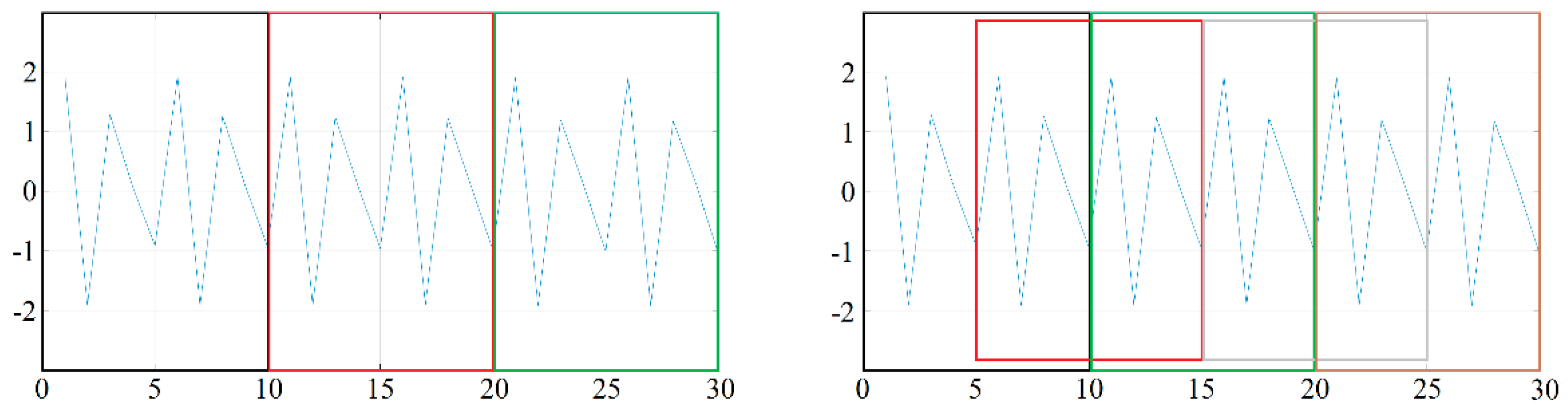
Segmentation can be done by simply breaking up the data stream (in which case, for example, a ten-second measurement is broken down into ten one-second pieces), but it can also be done using a sliding window, in which case there is some overlap between the data in successive windows. Of course, in the latter case, depending on the degree of overlap between the windows, we obtain a larger number of training (and test) samples. The difference between the two methods is illustrated in Figure 2. In the case of both methods, the same 30-item data set was segmented using a window size of 10, but the windows on the left side of the figure followed each other, so we finally obtained 3 samples, while on the right side, we used sliding windows with 50% overlap, and thus 5 samples were obtained. In the latter case, the samples follow each other in the order of black, red, green, gray, and brown.

Figure 2. Segmentation methods. Non-overlapping segments on the left and 50% overlapping segments on the right.

The greater the overlap, the more samples can be used for training; however, in the case of excessive overlap, successive windows provide only minimal extra information relative to each other, resulting in minimal contribution to improving the accuracy of the machine learning algorithm; meanwhile, the training time increases significantly.

The size of the segmentation window typically covers an interval of a few seconds [33,34,35]. It is important to choose the proper window size, because there is an optimal value that can maximize the performance of the model for a given machine learning task. With a window size smaller than this, the window may not contain enough information about the activity performed, which reduces the accuracy of the classification. Furthermore, for large window sizes, it can contain data from several different activities, especially if activity changes are relatively frequent. Although the latter problem can be more easily remedied by discarding windows that have undergone a change of activity, having too many can lead to a significant reduction in the number of training samples available. Another problem caused by the excessively large window occurs in real-time activity recognition: the result of the classification appears on the output with a larger delay after the activity change, and the output is not reliable during this time.

In our research, we tried to determine the ideal window size using the PhysioNet database. Data were segmented with different window sizes. The windows were almost completely overlapping, with an N-sized window containing the current and previous N-1 measurement points from data from the previously mentioned 16 EEG channels.

4.2. Neural Network

As discussed earlier, when recognizing activity from EEG data, the selection of the optimal learning algorithm and its appropriate parameterization are far from clear, and the various studies cited reached conflicting conclusions in many cases. At the same time, there is a trend that convolutional neural networks are gaining ground among the methods used in this type of activity recognition task. Based on these observations, we used a convolutional neural network as machine learning method. Feature extraction—also based on the conclusions of the cited articles—was entrusted to the network. Convolution—implemented by convolutional layers—plays a significant role in the extraction of features. If f and g are integrable functions defined in the range (-∞, ∞), then their convolution is the function defined by the following integral:

$$\left(f\ast g\right)\left(x\right)={{\displaystyle \int }}_{-\infty }^{\infty }f\left(t\right)g\left(x-t\right)dt.$$

(1)

Since the data is available in digital form, the discrete-time form of convolution, the convolution sum is applicable in our case:

$$\left(f\ast g\right)\left[n\right]={\displaystyle \sum }_{m=-\infty }^{\infty }f\left[m\right]g\left[n-m\right].$$

(2)

Convolutional neural networks are typically capable of processing image data, which are two-dimensional data structures. Of course, other types of input can also be interpreted as a kind of image, e.g., the EEG data, where the rows are given by the channels and the columns by the measurement points. Due to the two-dimensional nature of the data, it is necessary to use two-dimensional convolution, which can be calculated from the following equation:

$$y\left[i,j\right]={\displaystyle \sum }_{m=-\infty }^{\infty }{\displaystyle \sum }_{n=-\infty }^{\infty }h\left[m,n\right]x\left[i-m,j-n\right],$$

(3)

where x is the input data matrix and h is the convolution kernel. As a result of this calculation, the size of the output data matrix will be smaller than the input. Padding can be used to prevent continuous shrinkage of the output matrix size.

In the case of CNN, accuracy is largely determined by the structure of the network and its various parameters (kernel number, kernel size, etc.), so we compared the performance of networks with different structures to find the optimal one for this task. Since there is no especially good way to determine the layers and parameters of a (convolutional) neural network, we rely on experience and experimentation to design the structure.

The first of the neural networks used (hereafter CNN1) is a purely convolutional network; i.e., it does not contain fully connected layers. Its structure is summarized in Table 3.

Table 3. CNN1 network structure.

Layer Number	Layer Type
1	Input layer (segment size dependent)
2	2D convolution layer (16 5 × 5 filters, stride: 2 × 2, with zero padding)
3	Batch normalization layer (16 channels)
4	Activation layer (ReLU)
5	2D convolution layer (32 5 × 5 filters, stride: 2 × 2, with zero padding)
6	Batch normalization layer (32 channels)
7	Activation layer (ReLU)
8	2D convolution layer (64 3 × 3 filters, stride: 2 × 2, with zero padding)
9	Batch normalization layer (64 channels)
10	Activation layer (ReLU)
11	2D convolution layer (64 2 × 8 filters, stride: 2 × 8, without padding)
12	Batch normalization layer (64 channels)
13	Flatten layer

Experiments using the CNN1 network were also performed using a network with a different structure (hereafter CNN2) that also has pooling and fully connected layers. The structure of this network is summarized in Table 4.

Table 4. CNN2 network structure.

Layer Number	Layer Type
1	Input layer (segment size dependent)
2	2D convolution layer (8 3 × 3 filters, stride: 1 × 1, with zero padding)
3	Activation layer (ReLU)
4	Maximum pooling layer (pool size: 2 × 2, stride: 2 × 2)
5	2D convolution layer (16 5 × 5 filters, stride: 1 × 1, without padding)
6	Activation layer (ReLU)
7	Maximum pooling layer (pool size: 2 × 2, stride: 2 × 2)
8	Flatten layer
9	Fully connected layer (64 neurons)
10	Activation layer (ReLU)
11	Fully connected layer (32 neurons)
12	Activation layer (ReLU)
13	Fully connected layer (3 neurons)
14	Activation layer (Softmax)

In the next network (hereafter CNN3), the size of the filters in all convolution layers was reduced from 5 × 5 to 3 × 3; in all other respects, the model is the same as CNN1. In case of the next model used (hereafter CNN4), we returned to the kernel size used in CNN1, but this time we examined the effect of deepening the network. The CNN1 network was basically supplemented with a block containing convolutional, batch normalization, and ReLU layers, as shown in Table 5.

Table 5. CNN4 network structure.

Layer Number	Layer Type
1	Input layer (segment size dependent)
2	2D convolution layer (8 5 × 5 filters, stride: 2 × 2, with zero padding)
3	Batch normalization layer (8 channels)
4	Activation layer (ReLU)
5	2D convolution layer (16 5 × 5 filters, stride: 2 × 2, with zero padding)
6	Batch normalization layer (16 channels)
7	Activation layer (ReLU)
8	2D convolution layer (32 5 × 5 filters, stride: 2 × 2, with zero padding)
9	Batch normalization layer (32 channels)
10	Activation layer (ReLU)
11	2D convolution layer (64 3 × 3 filters, stride: 2 × 2, with zero padding)
12	Batch normalization layer (64 channels)
13	Activation layer (ReLU)
14	2D convolution layer (64 2 × 8 filters, stride: 2 × 8, without padding)
15	Batch normalization layer (64 channels)
13	Flatten layer

Training and testing were performed on a balanced data set, using data from 10 and 20 subjects. The applied algorithm was Adam Optimizer. Overall, 70% of the available data was used for training and 30% for testing.

5. Results

For the first time, we used a window size of 32 samples (0.2 s), with which we achieved a recognition accuracy of 79.2% on the 10-subject dataset. The values for each class are given in Table 6. It can be observed that the network confuses active activities with each other to a much lesser extent than with the relaxation.

Table 6. CNN1 confusion matrix for 10 subjects and segment size of 32.

		Predicted Class
		Hands	Feet	Relax
True class	Hands	32,501	3299	6120
	Feet	2292	34,253	4847
	Relax	4215	5245	32,280

We performed the same experiment on the 20-subject dataset, and the results obtained confirmed our previous hypothesis and the conclusion of [36], i.e., that these kind of brain activities vary from individual to individual. The overall result was 71.8%, which is significantly lower than the performance of the network with 10 subjects. The accuracy of the network was found to be unsatisfactory with such a small window size, but with a segment size of 64 (0.4 s), this greatly improved; the accuracy increased to 91.1% for 10 people and 83.3% for 20 people. By further increasing the size of the segments to 128 samples (0.8 s), even better classification results were obtained: 96.8% (10 individuals) and 94.6% (20 individuals). We have found that at this window size, there is no longer a significant difference between the results available on the two datasets. The last window size used was 160, which covers 1 s and causes such a delay for real-time data processing, so we did not want to increase it further. The classification accuracy was 99.1% for 10 and 97.7% for 20 subjects. The results were interpreted as follows: a segment of this size already contained enough individual independent information to allow the machine learning model to recognize a general pattern in the data.

The same experiments using CNN2 produced significantly worse accuracy. The data in Table 7 show that for any window size, the accuracy of CNN2 lags behind the accuracy of CNN1. On average, in all cases, performance of this network was nearly 20 percentage points lower than the previous one.

Table 7. Accuracy on PhysioNet data for 10/20 subjects.

Network	Segment Size (Number of Samples and Duration)
	32 (0.2 s)	64 (0.4 s)	128 (0.8 s)	160 (1 s)
CNN1	79.2%/71.8%	91.1%/83.3%	96.8%/94.6%	99.1%/97.7%
CNN2	62.5%/58.4%	62.1%/64%	76.4%/74.4%	82.6%/76.4%
CNN3	76.5%/68.6%	87.8%/80.2%	96.4%/91.2%	97.7%/93.6%
CNN4	76.2%/70.4%	86.1%/79.8%	96.9%/92.9%	99%/96.1%

Since CNN1 provided a much better classification result than CNN2, by using CNN3, we basically returned to the purely convolutional structure of CNN1. The CNN3 network uses a different approach, where the size of the filters in all convolution layers was reduced from 5 × 5 to 3 × 3. Apart from this, CNN3 is identical to CNN1 in all other aspects, as shown earlier. The accuracy obtained with this network is also summarized in Table 7. The results show that in terms of classification performance, this network is located between CNN1 and CNN2, lagging behind CNN1 by about 3 percentage points and significantly outperforming CNN2. In conclusion, with these data, using this CNN1/CNN3 network layer order, the 5 × 5 kernel size is more favorable than the 3 × 3.

Based on this experience, we developed the following applied model, which uses the kernel size as CNN1, but this time, we examined the effect of deepening the network. The same experiments were performed with this CNN4 model as with the previous ones.

The results obtained using different window sizes with different networks are summarized in Table 7 for both the 10- and 20-person data sets.

The data in the table show that there is a strong positive correlation between segment size and network classification accuracy; i.e., by increasing the segment size, the performance of the machine learning model significantly increases, regardless of which network we use. It can also be stated that the performance of CNN2, which does not include batch normalization but pooling and fully connected layers, has always been significantly lower than the performance of the other networks.

In terms of the effect of the kernel size, CNN1 using the 5 × 5 size performed slightly better in all cases than CNN3 using the 3 × 3 kernel. Although, as written in [37], the ideal kernel size varies from person to person, and may even be different from time to time for a given person. It can be stated that when looking for a solution that can be generalized to more people, with this neural network structure, the larger filter is the better choice.

Regarding the depth of the network, it can be stated that the use of a deeper network is not necessarily more advantageous than a shallower one. A network with more convolutions could theoretically obtain more relevant features, thus providing better classification performance. The counterargument is that due to having more parameters, it takes more time to train and is more prone to overfitting, which results in a less generalizable model. The data in the table show that the shallower CNN1 performed better in this task than the deeper CNN4.

The accuracy we achieved is higher than in the case of the work of other researchers. On the same database, also using the data of 20 people, we achieved a better result (97.7%) than the 93.86% reported in article [38]. Paper [39] used a dataset of 10 people, and their reported accuracy of 96.36% falls short of the 99.1% we achieved.

6. Hardware Implementation

In the Xilinx University Program, we were donated an Alveo U50 accelerator card that can be used to accelerate the pattern recognition speed of neural networks, among other things. As the next step in our research, we examined the possibility of hardware acceleration of neural networks using a deep learning processing unit (DPU) that can be implemented on this accelerator card. The card includes a unique UltraScale + FPGA that works exclusively on the Alveo architecture [40].

For development on an Alveo card, the manufacturer provides the Vitis AI environment, which can be used to accelerate the machine learning model. In order to operate the already-trained neural network on the Alveo card, a few process steps are required. The first of these is the creation of the frozen graph of the model. For most frameworks, the model created contains information (e.g., gradient values) that allows the model to be reloaded and, for example, resume the training from where it left off, but these are not required for inference. This step removes this type of information, but keeps the important ones, such as the structure of the graph itself, weights, etc., and saves them to a special file in Google Protocol Buffer (.pb) format.

The DPU can only perform fixed-point operations, so the next step is to convert the 32-bit floating-point values of the frozen graph to 8-bit integers. The fixed-point model requires lower memory bandwidth and provides higher speed and energy efficiency than the floating-point model. The quantization calibration process requires unlabeled input data (a few thousand samples), which the quantizer uses to analyze the distribution of values so that it can adapt dynamically. During quantization, the accuracy decreases somewhat for obvious reasons, but the calibration process does not allow it to be too high. The negative effect of quantization on recognition accuracy is summarized in Table 8. The study was performed on the 20-person dataset using a window size of 160 samples. It can be seen that the method caused an average decrease of 2.7 percentage points in the recognition accuracy compared to the results obtained using the floating-point numbers in the listed cases.

Table 8. Effect of quantization.

Neural Network	Accuracy (Floating-Point Model)	Accuracy (Fixed-Point Model)
CNN1	97.7%	94.7%
CNN2	76.4%	73.8%
CNN3	93.6%	90.4%
CNN4	96.1%	94.2%

Once the quantized model is available, it can be compiled into the instruction set of the applied DPU using the Vitis AI compiler framework. After analyzing the topology of the model, the compiler creates an internal computational graph as an intermediate representation and performs various optimizations, and then generates the compiled model based on the DPU microarchitecture. The DPUv3E is a programmable engine optimized for convolutional neural networks that can execute the instructions of the special instruction set of Vitis AI and thus enable the efficient implementation of many convolutional networks. The DPU is available as an IP (intellectual property) that can be implemented in the FPGA of the Alveo card. The operations it supports include convolution, deconvolution, pooling (both maximum and average), support for the ReLU function, and batch normalization, among others [41].

Running the inference on the Alveo card, we examined the speed advantage over running it on the CPU. The processor used was an Intel Core i7-9700KF and the system memory was 64 GB, with which we managed to perform an average of 5271.5 frame per second, while with the Alveo card, we achieved a recognition speed of 29339.9 frames per second. This is a significant difference in favor of Alveo, but we must also take into account the loss of accuracy due to quantization. Considering this, the use of an accelerator card in this specific application is not advantageous, since even in the case of real-time inference, the frequency of incoming data remains well below the level that can be handled by the CPU. However, in other applications, this DPU approach has significant potential. In a much more complex neural network than the one we use, pattern recognition can be very time consuming, so incoming data intensity can exceed the maximum that can be handled by the processor. In this case, the use of an accelerator card may be a solution, even if it is somewhat detrimental to accuracy.

7. Conclusions

In this paper, we proposed a convolutional neural network-based EEG motor imagery classification method to further improve the accuracy of pattern recognition. We examined the effect of the segment size and different neural network structures. We found positive correlation between segment size and network classification accuracy. Arguments can be listed for both shorter and longer window sizes; however, in comparing them, we found that a one-second window size is the optimal choice in this application. This provides a significant improvement over smaller window sizes in terms of recognition accuracy, while the delay it causes was found to be acceptable.

The results demonstrated that the performance of different network structures can differ significantly, and a deeper network does not necessarily provide a better result than a shallower one; however, it has drawbacks, for example, in terms of training time. Our results confirm that the automatic feature extraction possibilities of convolutional networks can be used well; with their help, high accuracy values can be achieved, and it is not necessary to perform time-consuming, manual feature extraction.

Regarding the hardware implementation of the network, we found the DPU-based approach somewhat reduces the accuracy due to the smaller bit-width representation, even with the use of quantization calibration, but exhibits variable performance in terms of inference rate. Consequently, this approach may be advantageous overall, but also disadvantageous for a given application.