Multi-Objective Multi-Learner Robot Trajectory Prediction Method for IoT Mobile Robot Systems

Abstract

Robot trajectory prediction is an essential part of building digital twin systems and ensuring the high-performance navigation of IoT mobile robots. In the study, a novel two-stage multi-objective multi-learner model is proposed for robot trajectory prediction. Five machine learning models are adopted as base learners, including autoregressive moving average, multi-layer perceptron, Elman neural network, deep echo state network, and long short-term memory. A non-dominated sorting genetic algorithm III is applied to automatically combine these base learners, generating an accurate and robust ensemble model. The proposed model is tested on several actual robot trajectory datasets and evaluated by several metrics. Moreover, different existing optimization algorithms are also applied to compare with the proposed model. The results demonstrate that the proposed model can achieve satisfactory accuracy and robustness for different datasets. It is suitable for the accurate prediction of robot trajectory.

1. Introduction

Mobile robots are one of the most important parts of the IoT system, which are capable of being automatic sensing nodes [1,2], flexible transportation carriers [3], or effective execution tools [4]. With the development of IoT technologies, the requirements for the stability of the mobile robot system are getting higher and higher [5]. As the core component of the IoT mobile robots, the positioning system often fails due to sensor failures or environmental interference [6]. The positioning failure and navigation error will cause a series of chain reactions, which will seriously affect the IoT environment [7].

The digital twin technology can fuse multi-source sensor data, construct a virtual model of the mobile robots, and monitor the health status of the robots in real time [8,9]. The focus of the digital twin system is on how to build a highly reliable virtual model [10]. According to the results of the virtual navigation model, the physical mobile robots can be aware of the difference between actual positions and expected positions [11]. Then, the mobile robot can reschedule to guarantee navigation performance. As for the digital twin system of robot navigation, the most important parameter is the navigation trajectory. The abnormalities in the robot navigation system can be reflected in the navigation trajectory [12]. If the robot deviates or sensors fail, the difference between the actual trajectory and virtual trajectory will be large [13]. Therefore, to provide virtue trajectory information for the digital twin systems for mobile robots, the robot trajectory prediction should be investigated [14].

1.1. Literature Review

In recent trajectory prediction studies, the data-driven methods are the mainstream, which can discover the underlying fluctuation rule of the robot trajectory from historical data [15]. The data-driven trajectory prediction models can be divided into statistical methods and intelligent methods. The commonly-used statistical methods contain the Kalman filter [16], autoregressive moving average (ARMA) [17], Gaussian process method [18], etc. The statistical methods have fast calculation speed and strong interpretability. However, the non-linear fitting performance is not sufficient, which limits the usage [19]. Compared with statistical methods, the intelligent methods, especially the deep learning method, have a stronger fitting and generalization capacity, and are more frequently used in recent studies [20]. For example, Seker et al. combined a convolutional neural network (CNN) and long short-term memory (LSTM) for robot trajectory prediction, which used the CNN to extract features of the trajectory time series, and applied the CNN to describe temporal dependency for prediction [21]. Li et al. applied a novel LSTM structure to predict positions and directions [22]. Zhang et al. used an RNN with Monte-Carlo dropout for trajectory prediction in human–robot interaction [23]. Nikhil et al. proposed a fast trajectory prediction method based on a compact CNN algorithm [24].

The above studies all proved the effectiveness of the intelligent trajectory prediction methods. They used diverse prediction methods to predict the robot’s trajectory. However, due to the diversity of the prediction mechanism, all prediction models have a different focus on learning features [25]. Considering the diverse characteristics of the robot trajectory, the learning scope of the single prediction model is limited, leading to limited application scenarios and prediction accuracy [26]. To overcome this drawback, a multi-learner strategy should be studied, which applies multiple learners to broaden the learning scope. To ensure diversity, the structure of the learners should be different [27]. In this study, three types of learners are applied, including linear regression, shallow neural works, and deep neural works. These three types of learners can focus on linear components, weak non-linear components, and strong non-linear components, respectively, to learn multifaceted features of the trajectory.

Given the multiple learners, how to combine them is one of the core problems to ensure effectiveness [28]. The combined model is expected to outperform any learner. The boosting, stacking, and optimization strategies are commonly used to combine multiple weak models into a strong ensemble model [29,30]. For example, Wang et al. applied adaptive boosting (AdaBoost) to combine multiple Markov models to improve spatial location prediction accuracy [31]. Rasouli et al. stacked several recurrent networks for trajectory prediction [32]. Xu et al. applied the particle swarm optimization gravitational search algorithm (PSOGSA) to calculate the ensemble weights of the spatial prediction models [33]. Although the above methods have been proved to be valid, they only consider the accuracy; the robustness of the ensemble model is not involved. The ensemble model with poor robustness is prone to overfitting, and has a strong dependency on the performance on the dataset [34]. Obviously, the one-sided pursuit of prediction accuracy will make it difficult for the model to show excellent performance on multiple different datasets. To solve the above-mentioned research gaps and take into account the accuracy and robustness comprehensively, the multi-objective optimization method should be investigated.

1.2. The Novelty of the Study

According to the above research gaps, a novel multi-objective multi-learner prediction (MMP) model is proposed for trajectory prediction. The ARMA, multi-layer perceptron (MLP), Elman neural network (ENN), deep echo state network (DESN), and LSTM are used as the weak learner. The ensemble weights can be obtained by non-dominated sorting genetic algorithm III (NSGA-III) to generate accurate and robust ensemble prediction results.

The scientific contributions of the study are presented as follows:

• A multi-objective multi-learner prediction structure is proposed for trajectory prediction. This model structure can fit the complex linear and non-linear components of the trajectory while ensuring accuracy and robustness simultaneously. The effectiveness of the proposed prediction model is validated with several real robot trajectories over several benchmark models.
• Previous studies only utilized a single model for trajectory prediction, which has a limited learning scope and cannot cope with complex components of trajectory. In this study, a multi-learner prediction method is proposed which uses ARMA, MLP, ENN, DESN, and LSTM for prediction. The ARMA can fit the linear components. The MLP and ENN can describe the weak non-linear components in a non-recursive and recursive manner, respectively. The DESN and LSTM can grasp strong non-linear components non-recursively and recursively. These diverse learners can achieve omnidirectional capture of trajectory features.
• The existing studies barely consider robustness when constructing an ensemble model, which makes the ensemble model prone to overfit and limited generalization performance. To mitigate the research gaps, an ensemble strategy based on the multi-objective optimization method is proposed. The multi-objective ensemble strategy can generate ensemble weights considering the accuracy and robustness simultaneously, leading to better comprehensive performance.

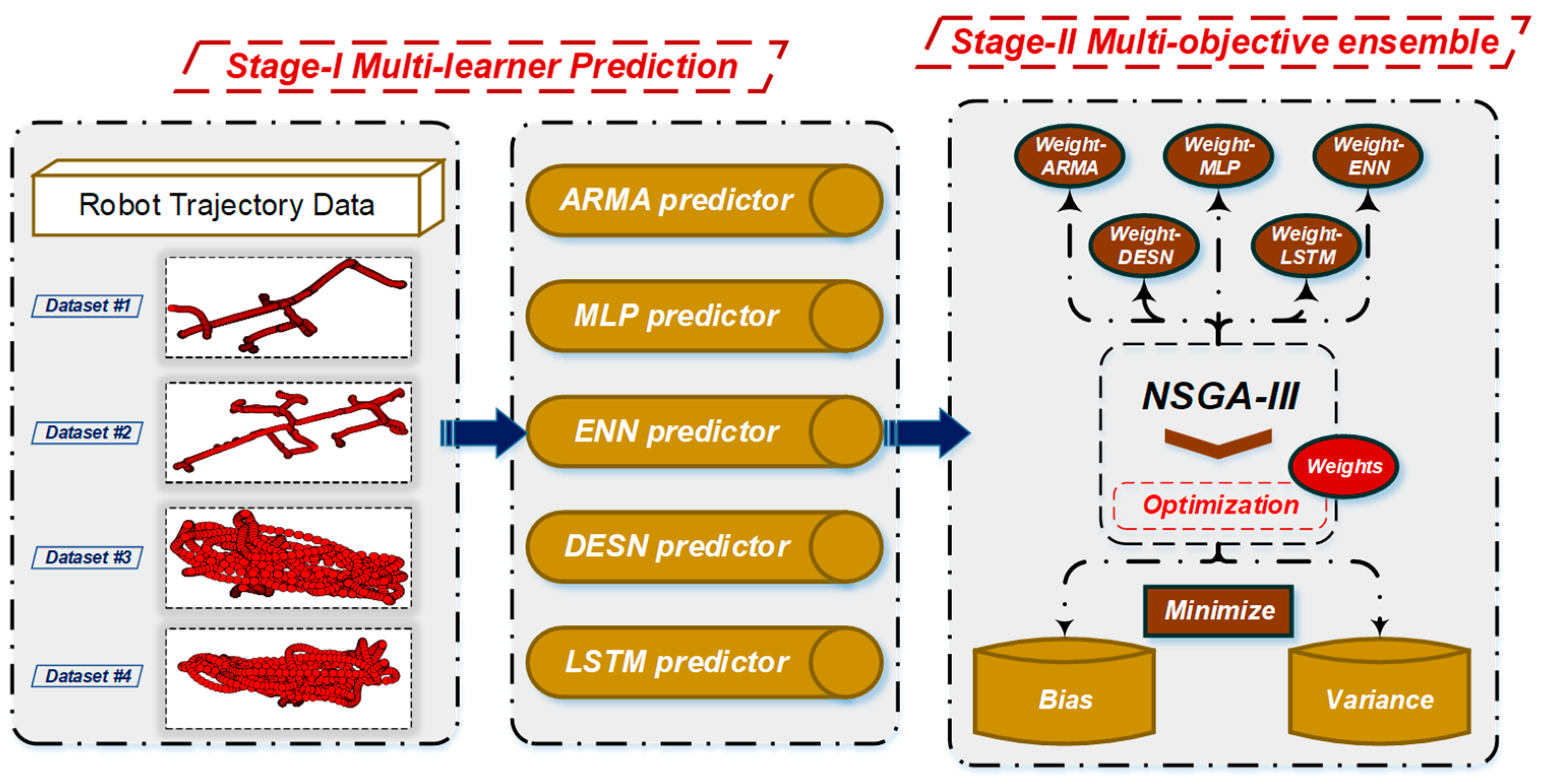
2. Methods

The proposed MMP model consists of two stages, namely multi-learner prediction and multi-objective ensemble. The specific framework of the proposed model is shown in Figure 1.

• Stage 1: multi-learner prediction. The trajectory dataset is divided into training and testing datasets. The trajectory is separated into several series in the orthogonal coordinate system. Fed with all orthogonal series, the ARMA, MLP, ENN, DESN, and LSTM are trained with the training dataset and generate forecasting results in the testing datasets.
• Stage 2: multi-objective optimization. The forecasting results of the multiple learners are combined by the NSGA-III to construct the ensemble model. Setting bias and variance as the objective function, the NSGA-III is applied to optimize the ensemble weights. Applying the obtained weights to the testing dataset, the ensemble forecasting results of the orthogonal series can be obtained. Synthesizing series forecasting results in the orthogonal coordinate system, the final deterministic trajectory forecasting results can be obtained.

2.1. Stage 1: Multi-Learner Prediction

An N-dimensional trajectory $Y=\left[y_1,y_2,\dots ,y_N\right]$ can be mapped into an orthogonal coordinate system and generate several orthogonal series. These orthogonal series are predicted individually in this study. The multiple learners are required to take series from each coordinate as input and to generate corresponding prediction results. The historical horizon and prediction horizon are denoted as H and L, respectively. In this study, the H and L are set according to Ref. [35]. The historical horizon H is set as 10, which is recognized to be able to produce better performance [35]. The prediction horizon L is set as 5 to study the long-term prediction performance [35]. Assuming a series of i-th orthogonal series as $y_i$, the input of the model is $\left[y_i\left(t-H+1\right),y_i\left(t-H+2\right),\dots ,y_i\left(t\right)\right]$ at time t, and the future values $\left[{\widehat{y}}_i\left(t+1\right),{\widehat{y}}_i\left(t+2\right),\dots ,{\widehat{y}}_i\left(t+L\right)\right]$ can be obtained with the model. The predicted trajectory $\widehat{Y}\left(t\right)=\left[\widehat{Y}\left(t+1\right),\widehat{Y}\left(t+2\right),\dots ,\widehat{Y}\left(t+L\right)\right]$ can be obtained by synthesizing all orthogonal series.

In this study, the ARMA, MLP, ENN, DESN, and LSTM are applied for prediction, and are briefly introduced as follows:

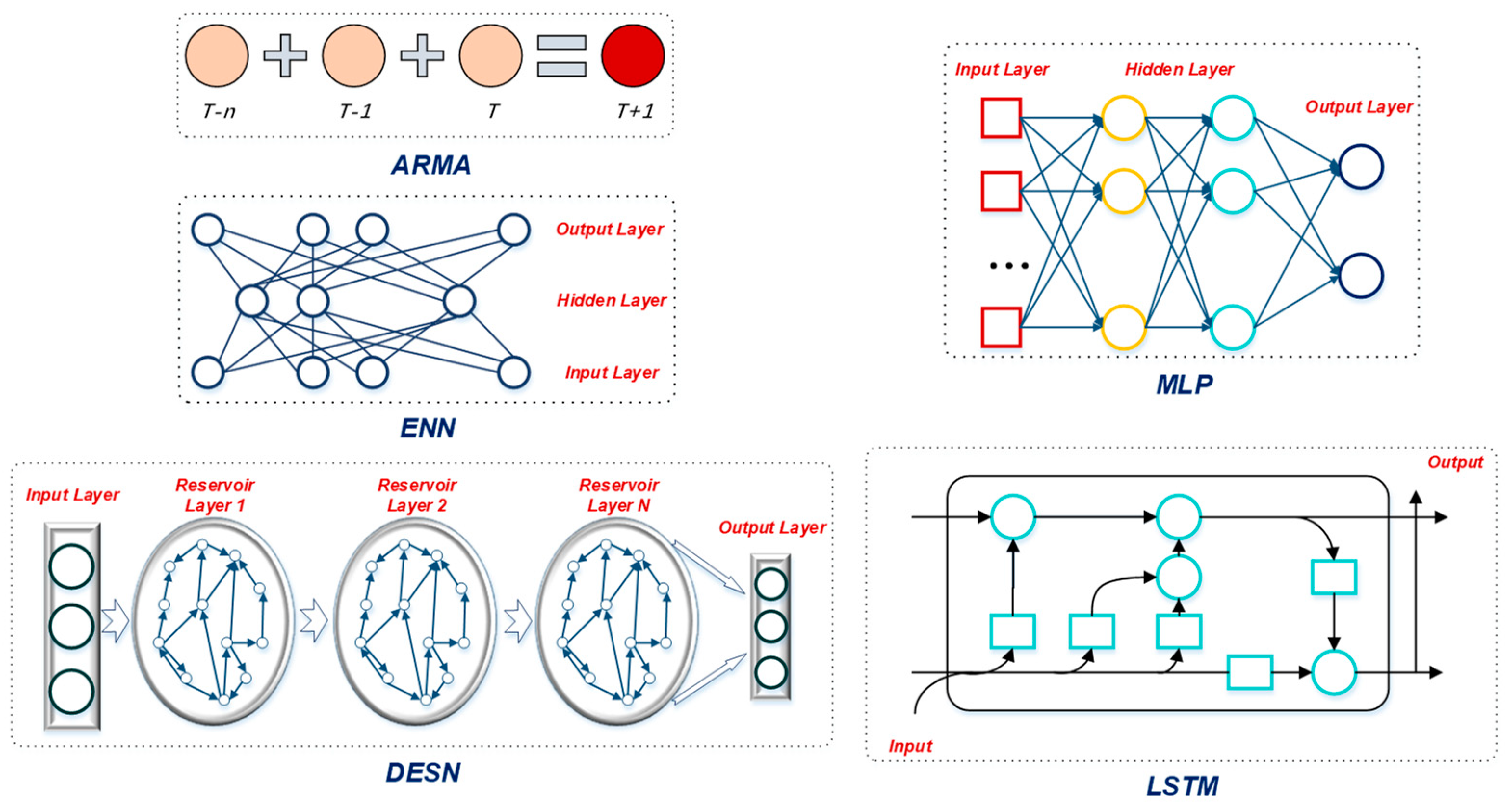
• The ARMA is a stochastic model in time series analysis, and can build regression equations through the correlation between data [36].
• The MLP is a feedforward artificial neural network, which can map multiple input datasets to output datasets [37].
• The ENN is a simple recurrent neural network, which consists of an input layer, a hidden layer, and an output layer; it has a context layer that feeds back the hidden layer outputs in the previous time steps [38].
• The DESN is the extension of the ESN (echo state network) approach to the deep learning framework, which is composed of multiple reservoir layers stacked on top of each other [39].
• The LSTM model is a kind of recurrent neural network; this model can address gradient exploration and vanishing problems during training [40].

These five models are widely used in time series forecasting problems and have diverse characteristics. The ARMA can fit the linear components. The MLP and ENN can describe the weak non-linear components in a non-recursive and recursive manner, respectively. The DESN and LSTM can grasp strong non-linear components non-recursively and recursively. The diverse characteristics of the models are understood to be able to facilize high-performance ensemble models [41].

With the generated input and output, the ARMA, MLP, ENN, DESN, and LSTM can be applied. These models can be trained with the training dataset and generate prediction results for testing datasets. Figure 2 shows the structure of each basic prediction model.

2.2. Stage 2: Multi-Objective Ensemble

NSGA-III [42] is an improved multi-objective optimization algorithm widely used in many fields. NSGA-III introduces a reference point mechanism based on NSGA-II, which uses the characteristics of distributed reference points in high-dimensional objects to maintain the diversity of populations. The main implementation steps of the NSGA-III can be interpreted as follows [42]:

• Generate reference points on the hyper-plane of the multi-objective functions.
• Normalize population members by constructing extreme points.
• Associate population members to the reference points, and carry out the niching-preserving operation to balance population member distribution.
• Execute genetic crossover and mutation operation to generate an offspring population.

This advantage makes NSGA-III have better algorithm convergence, and it is not easy to fall into the local optimum. The method of constructing weights by boundary crossing is used to preset a set of search target directions that can cross the Pareto surface to iteratively obtain the solution set distributed in the Pareto optimal front [43].

With the predicted trajectories of the multiple learners, the ensemble weights should be calculated with comprehensive consideration of accuracy and robustness. The accuracy means the prediction results have small deviations from the actual trajectory. The robustness means the prediction model does not rely on the training data. To measure the accuracy and robustness, the bias and variance are presented as follows [44]:

$$\{\begin{array}{c}Bias=E_t\left[{\left(E_D\left[\widehat{Y}\left(t;D\right)\right]-E_{\epsilon }\left[Y\left(t;\epsilon \right)\right]\right)}^2\right]\\ Variance=E_{t,D}\left[{\left(\widehat{Y}\left(t;D\right)-E_D\left[\widehat{Y}\left(t;D\right)\right]\right)}^2\right]\end{array}$$

(1)

where $\widehat{Y}\left(t;D\right)$ is the predicted trajectory at time t where the prediction model is trained with samples D. The training sample D is selected from the training dataset in the cross-validation manner. The actual trajectory $Y\left(t;\epsilon \right)$ is composed of real trajectory and disturbance $\epsilon$. $Y\left(t\right)=E_{\epsilon }\left[Y\left(t;\epsilon \right)\right]$ is the real trajectory without disturbance $\epsilon$. Because the disturbance $\epsilon$ is unmeasurable, the real trajectory $Y\left(t\right)$ without disturbance cannot be measured. In this study, the $E_{\epsilon }\left[Y\left(t;\epsilon \right)\right]$ is estimated as $Y\left(t;\epsilon \right)$. $E_D$ and $E_t$ are the expectations of the trajectory on times and training datasets.

With the bias and variance formula, the objective functions can be obtained as follows:

$$\begin{array}{c}\{E_t\left[{\left(E_D\left[\widehat{Y}\left(t,D\right)\right]-Y\left(t,\epsilon \right)\right)}^2\right],E_{D,t}\left[{\left(\widehat{Y}\left(t,D\right)-E_D\left[\widehat{Y}\left(t,D\right)\right]\right)}^2\right]\}\\ \begin{array}{cc}\mathrm{s}.\mathrm{t}.& \widehat{Y}\left(t,D\right)=\frac{{\displaystyle {\sum }_i{\widehat{Y}}_i\left(t,D\right)w_i}}{{\displaystyle {\sum }_i{w}_i}}\\ & 0\le w_i^{}\le 1\end{array}\end{array}$$

(2)

where $w_i$ is the i-th ensemble weight and ${\widehat{Y}}_i\left(t,D\right)$ is the predicted trajectory of i-th model.

In this study, the NSGA-III is applied to solve the multi-objective optimization, and a Pareto front can be generated. The work of many researchers has shown that calculating the combined weights of models through multi-objective optimization is a very effective solution to improve the performance of prediction models [45,46,47]. It is worth mentioning that the VIKOR (VlseKriterijumska Optimizacija I Kompromisno Resenje) [48], TOPSIS (technique for order of preference by similarity to ideal solution) [49], and Gray correlation methods [50] are used to solve Pareto optimal solutions $w^{best}$. The prediction results on the testing dataset can be obtained as follows:

$${\widehat{Y}}^{test}\left(t\right)=\frac{{\displaystyle {\sum }_i{E}_D\left({\widehat{Y}}_i^{test}\left(t,D\right)\right)w_i^{best}}}{{\displaystyle {\sum }_i{w}_i^{best}}}$$

(3)

where ${\widehat{Y}}_i^{test}\left(t,D\right)$ is the predicted trajectory on the testing dataset at time t where the model is trained with samples D and ${\widehat{Y}}^{test}\left(t\right)$ is the final deterministic predicted trajectory at time t on the testing dataset.

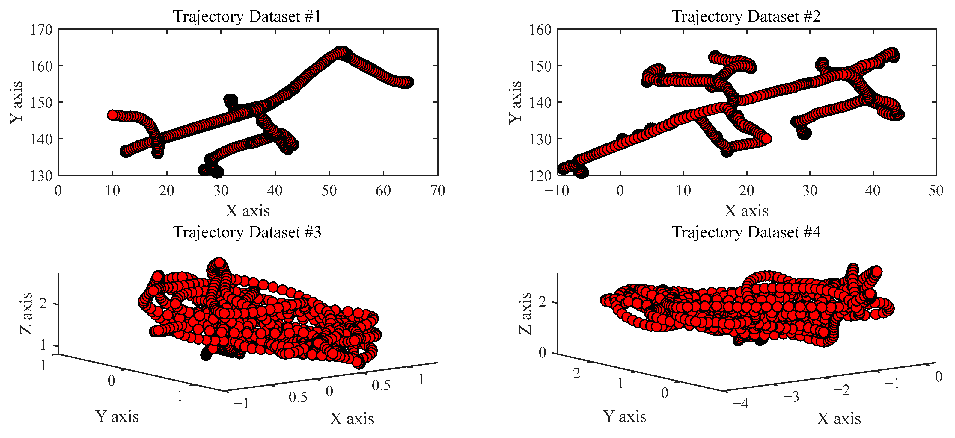
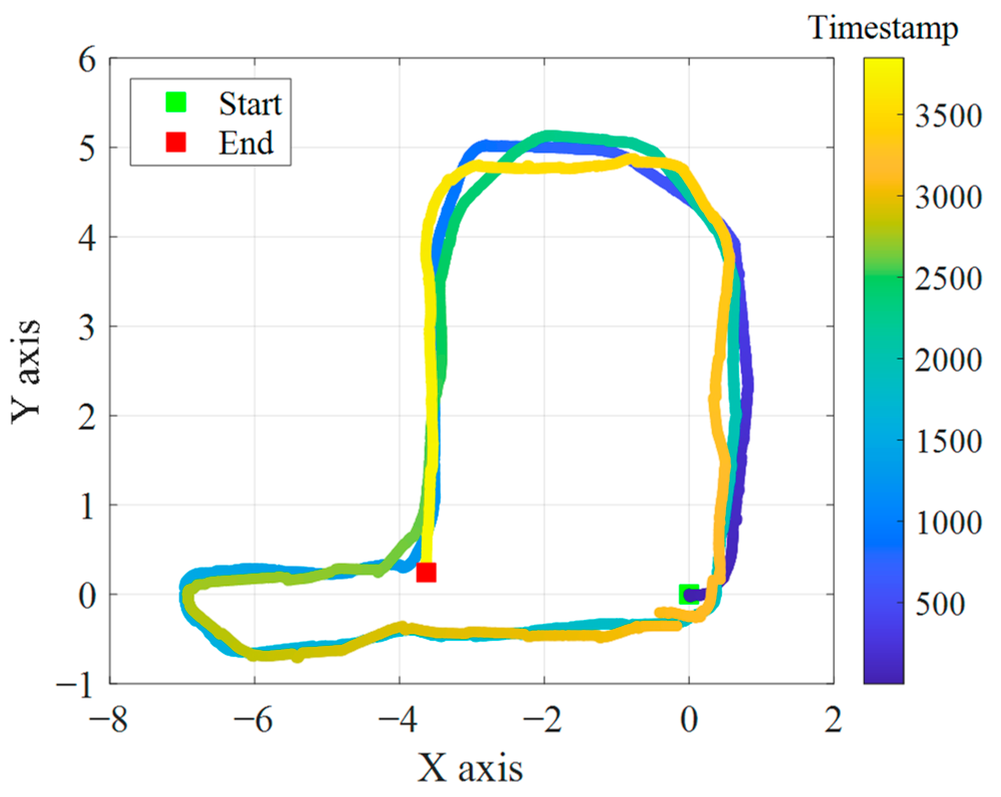
2.3. Data Description

In this study, four trajectories are applied to validate the prediction performance of the proposed model. The MIT Stata Center Data Set is used for experimental validation of two-dimensional predictions (https://projects.csail.mit.edu/stata/ (accessed on 24 April 2022)). The dataset includes more than 2.3 TB and 42 km of recorded data. In this paper, two ground truth trajectories of the dataset are taken as the first and second data for experiments. The sampling frequency of trajectory datasets #1 and #2 is 20 Hz, that is, the sampling period is 0.05 s (horizon = 0.05 s).

In addition to the two-dimension trajectory, the performance of the proposed method on the three-dimension trajectory should be investigated for stereo IoT. The third and fourth trajectories are collected by a three-dimensional motion capture system of the micro aerial vehicle (MAV) under different smart home environments (http://wbli.me/lmdata/ (accessed on 1 August 2021)). The sampling frequency of trajectory datasets #3 and #4 is 10 Hz, that is, the sampling period is 0.1 s (horizon = 0.1 s). The details about the MAV trajectories can be found in Ref. [51].

The trajectories utilized in this study are shown in Figure 3. Each of the trajectories has 1000 data points. The first 700 data points are utilized as the training set and the remaining 300 data points are utilized as the testing set. It can be observed that trajectory datasets #1 and #2 are two-dimensional, while datasets #3 and #4 are three-dimensional, with which we can verify the performance of the model comprehensively. It is worth mentioning that the number of advance prediction steps for each constructed model is five steps, and the prediction timestep windows are the same as the prediction horizons.

2.4. Evaluation Metrics

The deterministic evaluation metrics of the trajectory prediction contain average displacement error (ADE) [52], non-linear average displacement error (NLADE) [53], and final displacement error (FDE) [54]. The equations of these metrics are shown as follows:

$$\{\begin{array}{c}ADE=\frac{1}{L\times n}{\displaystyle \sum _i^L{\displaystyle \sum _j^n{\Vert {\widehat{Y}}_{}^{i,j}-Y_{}^{i,j}\Vert }_2}}\\ NLADE=\frac{1}{L\times n}{\displaystyle \sum _i^L{\displaystyle \sum _j^{n}I\left(Y_{}^{i,j}\right){\Vert {\widehat{Y}}_{}^{i,j}-Y_{}^{i,j}\Vert }_2}}\\ FDE=\frac{1}{n}{\displaystyle \sum _j^n{\Vert {\widehat{Y}}_{}^{L,j}-Y_{}^{L,j}\Vert }_2}\end{array}$$

(4)

where ${\widehat{Y}}_{}^{i,j}$ and $Y_{}^{i,j}$ are the j-th predicted and real trajectory locations of i-step ahead prediction, respectively. $I\left(Y_{}^{i,j}\right)$ is the indicator for the second derivative, which can be presented as follows:

$$I\left(Y_{}^{i,j}\right)=\{\begin{array}{cc}1& \frac{d^2{y}_1^{i,j}}{d^2{y}_2^{i,j}}\ne 0\\ 0& else\end{array}$$

(5)

where $y_1^{i,j}$ and $y_2^{i,j}$ are the 1st and 2nd dimensions of the trajectory, respectively. The definition of $I\left(Y_{}^{i,j}\right)$ enables the NLADE to measure the error in the non-linear trajectory.

3. Results and Discussions

3.1. Multi-Learner Prediction

With the ARMA, MLP, ENN, DESN, and LSTM, the prediction results can be obtained. The five-step ahead prediction results for dataset #1, dataset #2, dataset #3, and dataset #4 are shown in Figure 4, Figure 5, Figure 6 and Figure 7. Moreover, the corresponding evaluation metrics are shown in

Table 1. Evaluation metrics of ARMA, MLP, ENN, DESN, and LSTM models.

Dataset	Model	ADE	NLADE	FDE
#1	ARMA	0.455	0.455	0.904
	MLP	0.580	0.580	1.084
	ENN	0.940	0.940	1.262
	DESN	0.364	0.364	0.730
	LSTM	1.160	1.160	1.954
#2	ARMA	1.485	1.485	2.487
	MLP	2.433	2.433	2.652
	ENN	4.879	4.879	7.583
	DESN	1.301	1.301	1.545
	LSTM	1.635	1.635	2.170
#3	ARMA	0.063	0.063	0.142
	MLP	0.060	0.060	0.116
	ENN	0.034	0.034	0.079
	DESN	0.033	0.033	0.076
	LSTM	0.064	0.064	0.123
#4	ARMA	0.096	0.097	0.216
	MLP	0.114	0.114	0.198
	ENN	0.071	0.071	0.165
	DESN	0.057	0.057	0.129
	LSTM	0.104	0.105	0.202

. According to Figure 4, Figure 5, Figure 6 and Figure 7 and Table 1, the following can be observed:

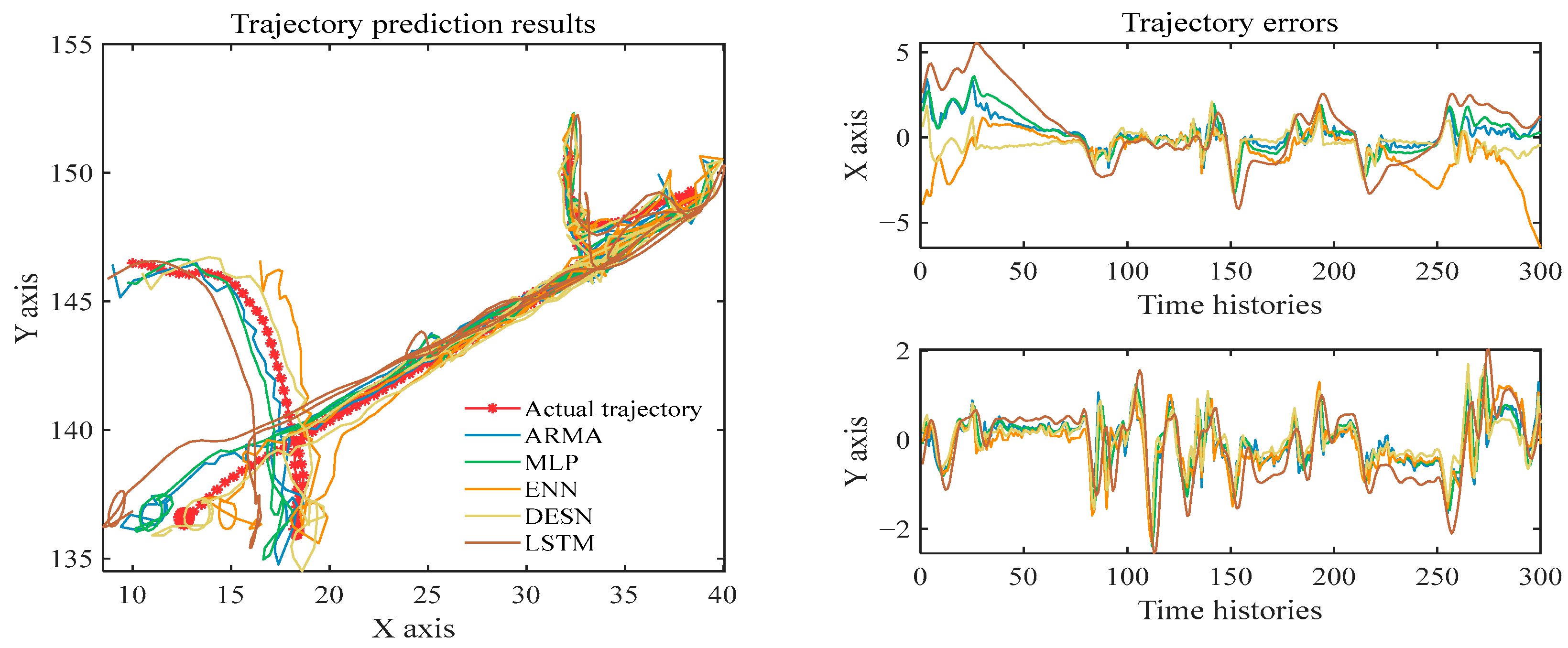
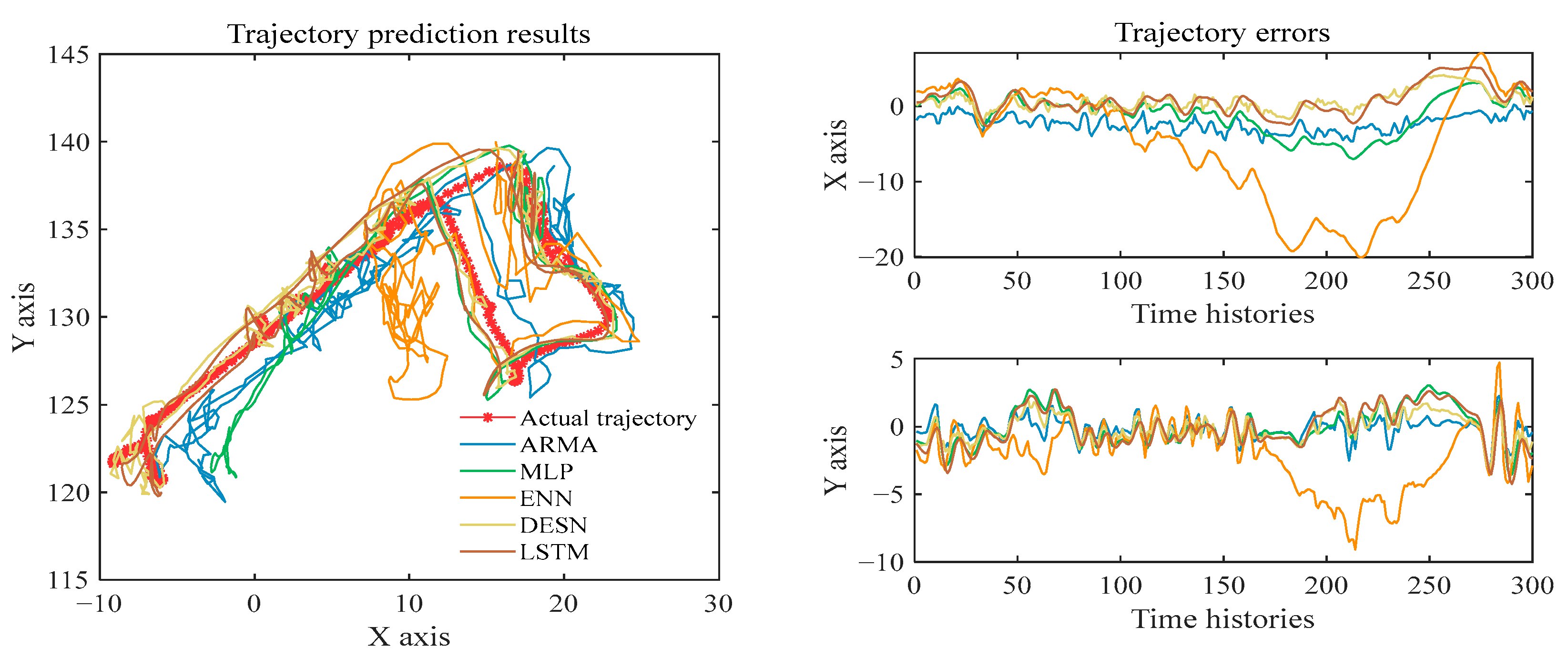
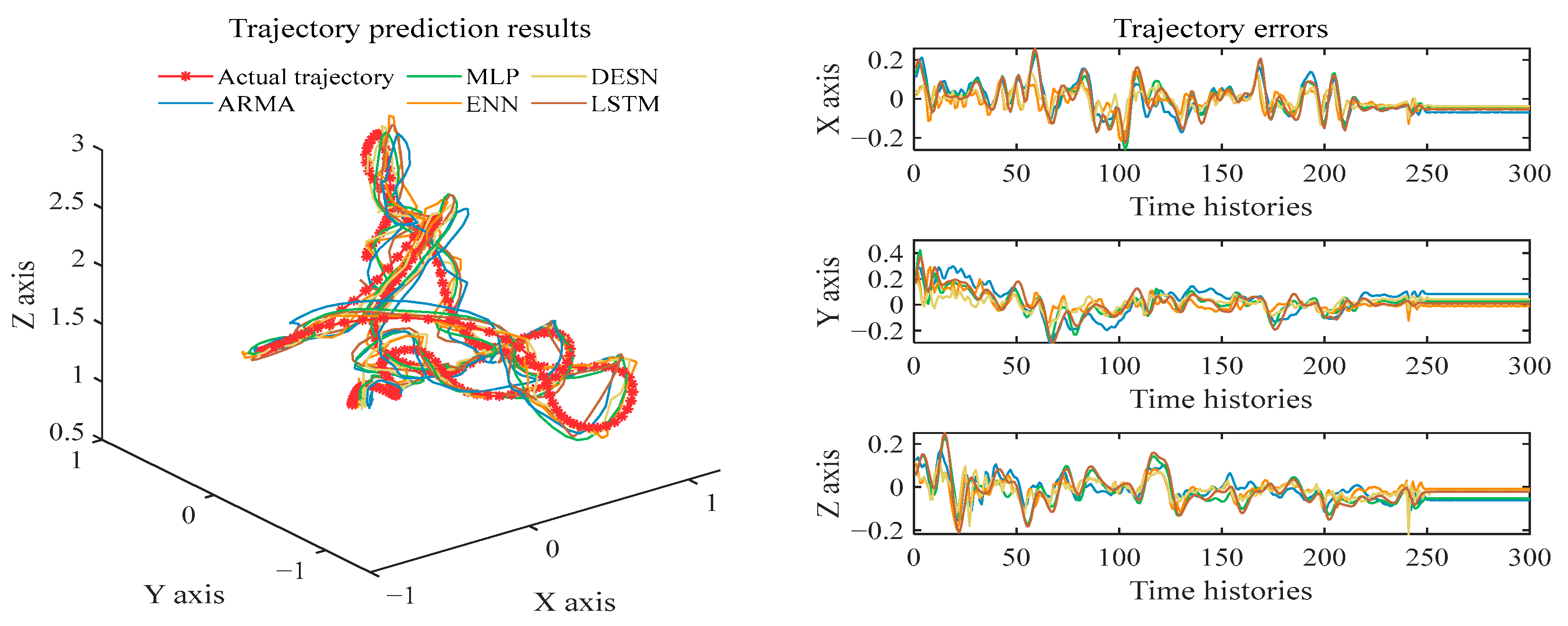
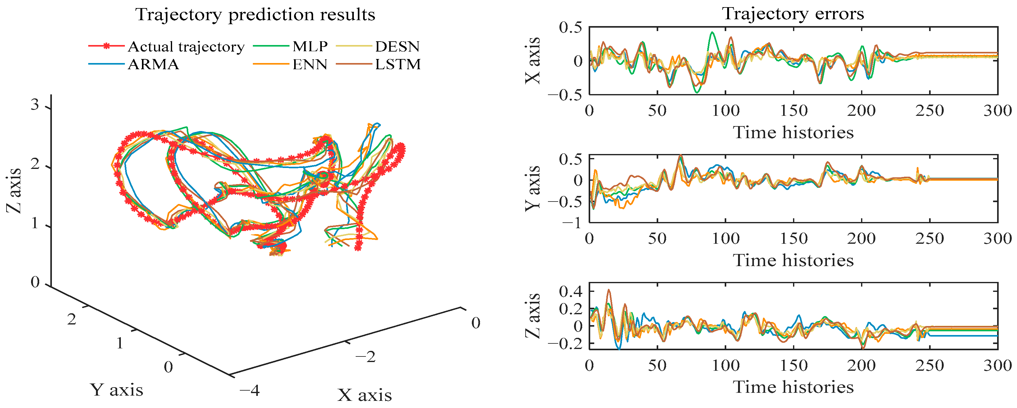
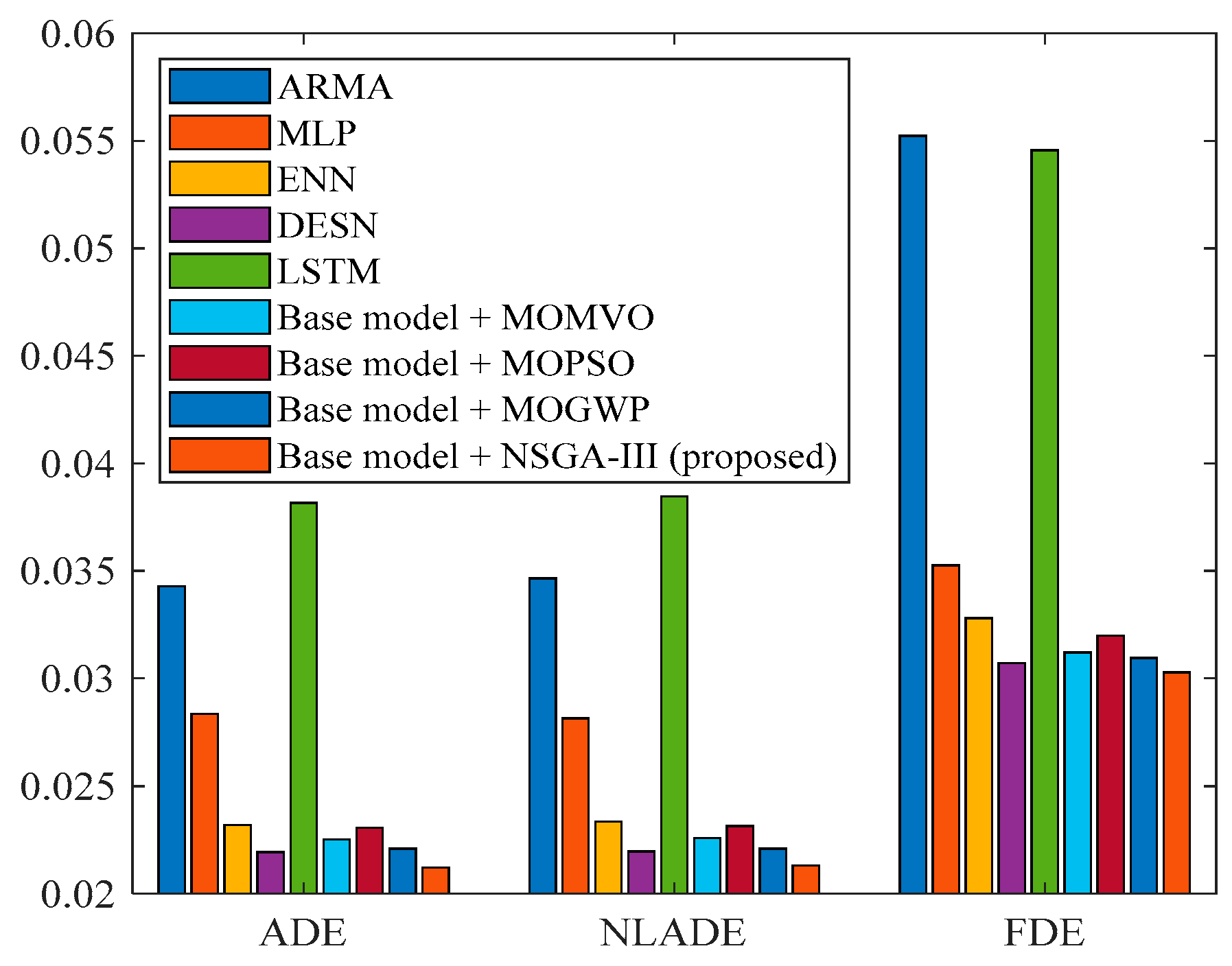
• The different base learners have various performances on robot trajectory prediction. For instance, the ADE values of the ARMA, MLP, ENN, DESN, and LSTM models are 0.455, 0.580, 0.940, 0.364, and 1.160 for dataset #1, respectively. The essential reason is the difference between model theories and parameters. Such differences contribute to the subsequent construction of multi-objective ensemble learning models, because ensemble learning requires that the base learners should be unique. Only in this way can more accurate prediction results be obtained through ensemble learning.
• Among all the base learners, the prediction error of DESN remains the lowest in the three datasets, and the prediction result of the trajectory is closer to the real trajectory. Taking the prediction result of dataset #4 as an example, the ADE, NLADE, and FDE of the DESN model are 0.057, 0.057, and 0.129, respectively. They are much lower than those of the other base learners. This phenomenon may be because the DESN benefits from its deep network structure and has a strong ability to learn sequential data such as robot trajectory.
• The prediction effects of ENN on the three datasets are significantly different. In dataset #2, the prediction error is the highest among the five models. However, it is second only to the DESN model in datasets #3 and 4. The instability of prediction results may be because ENN is sensitive to data and parameters. It is difficult to obtain satisfactory results for all data without parameter tuning.

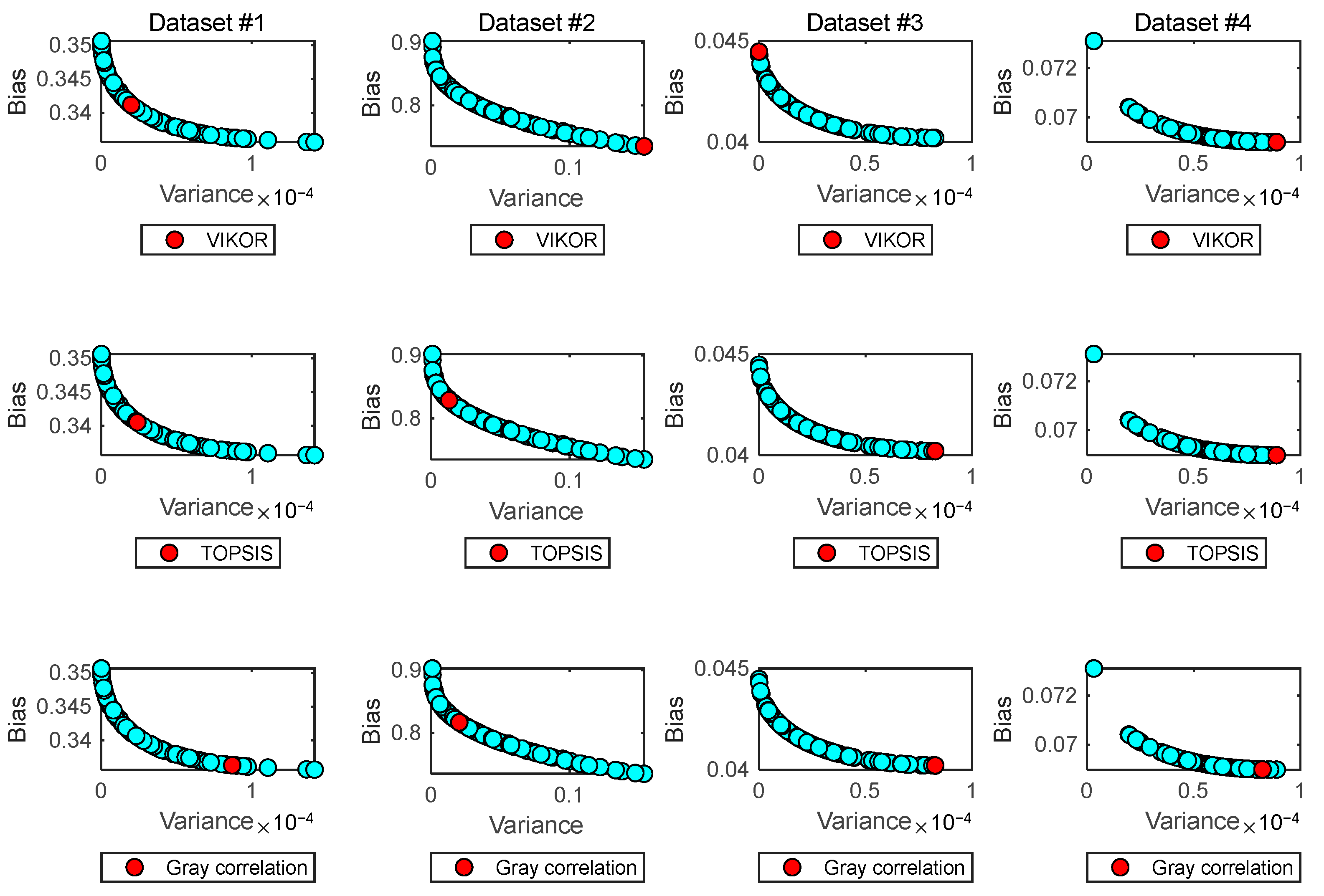
3.2. Multi-Objective Ensemble

Applying the NSGA-III to generate the optimal ensemble weights, the prediction results of the proposed MMP model can be obtained. The Pareto optimal solutions obtained by different optimization methods are different, which leads to differences in the prediction errors of the models. The related evaluation metrics in

Table 2. Evaluation metrics of the proposed MMP model.

Dataset	Optimization Method	ADE	NLADE	FDE
#1	VIKOR	0.346	0.346	0.685
	TOPSIS	0.347	0.347	0.687
	Gray correlation	0.347	0.347	0.688
#2	VIKOR	0.783	0.783	1.425
	TOPSIS	0.946	0.946	1.700
	Gray correlation	0.916	0.916	1.668
#3	VIKOR	0.032	0.032	0.073
	TOPSIS	0.029	0.029	0.068
	Gray correlation	0.029	0.029	0.068
#4	VIKOR	0.052	0.052	0.119
	TOPSIS	0.052	0.052	0.119
	Gray correlation	0.051	0.051	0.118

show the results of several methods for solving Pareto optimality, including VIKOR [48], TOPSIS [49], and Gray correlation [50]. In addition, Figure 8 shows the Pareto optimal results solved by the above methods. The bold numbers in Table 2 indicate the best solving method with the lowest prediction error among VIKOR, TOPSIS, and Gray correlation for datasets #1, 2, 3, and 4. The red points in Figure 8 represent the comprehensive optimal solution considering both bias and variance. It can be seen that there is no best strategy to select optimal ensemble weights. In datasets #1 and 2, the VIKOR generates the best performance. In dataset #3, the TOPSIS and Gray correlation select the same solution and both generate the best performance. In dataset #4, the Gray correlation generates the best performance.

Comparing Table 2 with Table 1, it can be observed that the overall accuracy of the ensemble model in Table 2 is better than that of the five base models in Table 1 for all datasets. Taking dataset #1 as an example, the best forecasting ADE of single models in Table 1 is 0.364. The ensemble models in Table 2 have a forecasting ADE of 0.346, 0.347, and 0.347, which are all better than that of the best single model in Table 1. This phenomenon indicates the proposed multi-objective ensemble can reasonably balance the bias and variance of prediction and help to synchronously minimize them to improve performance.

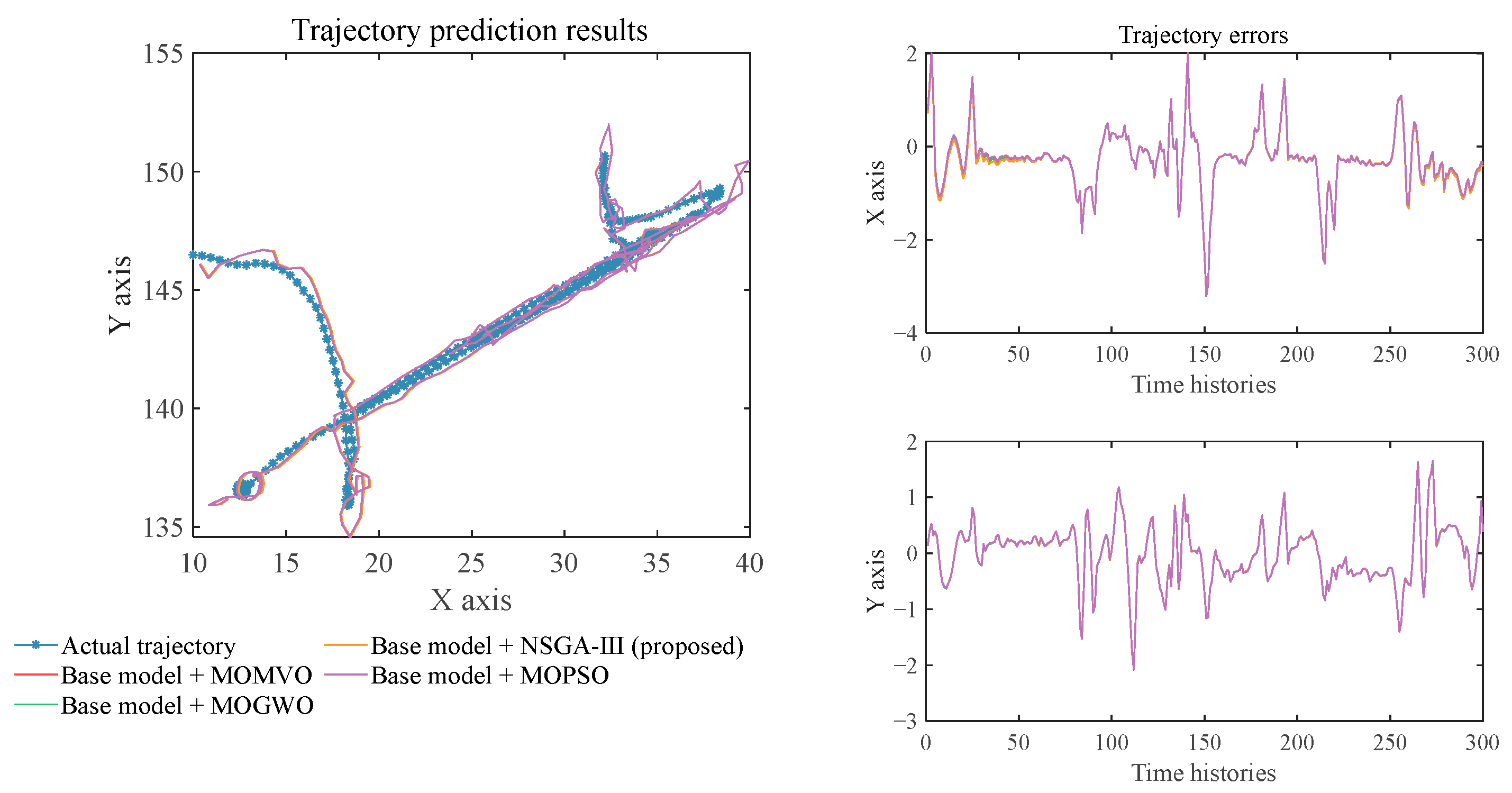
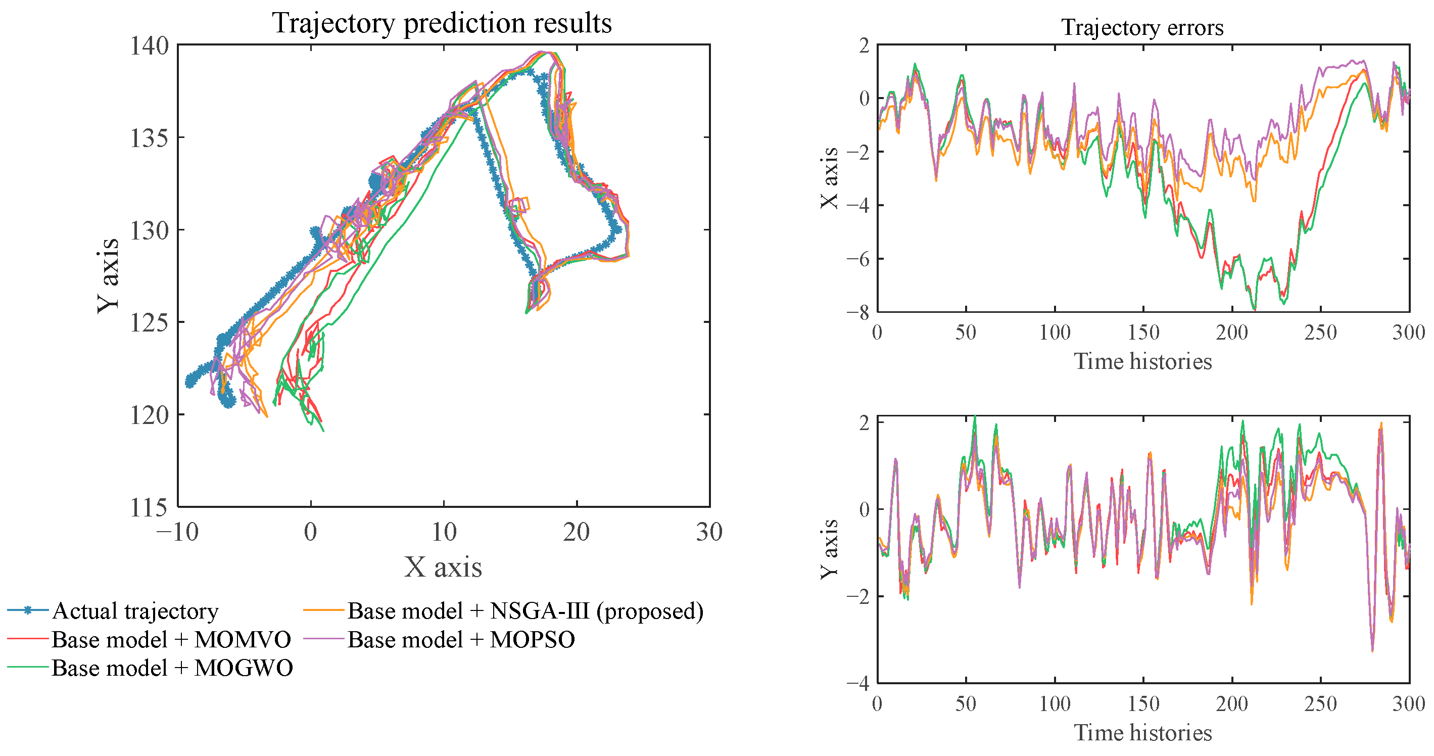
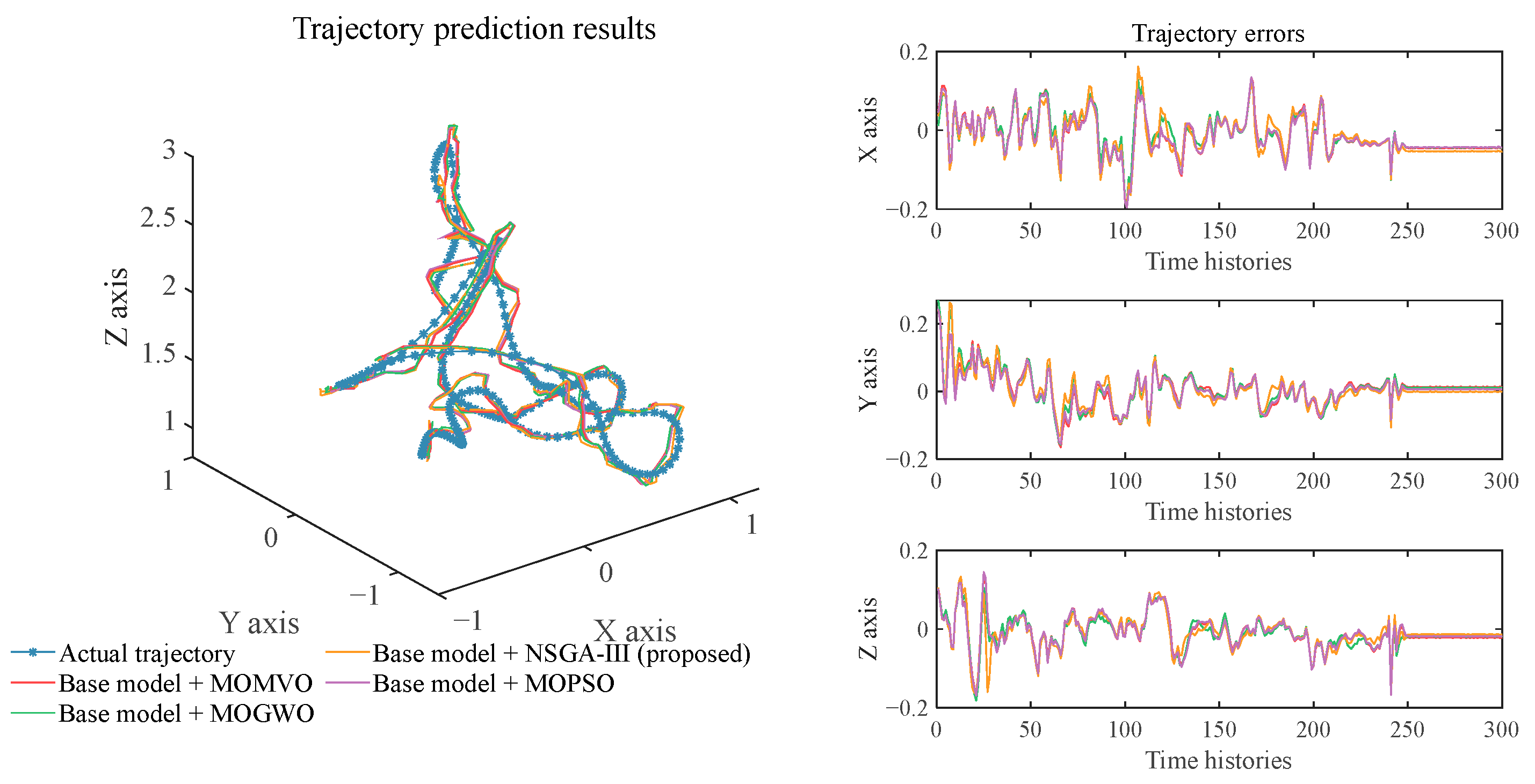
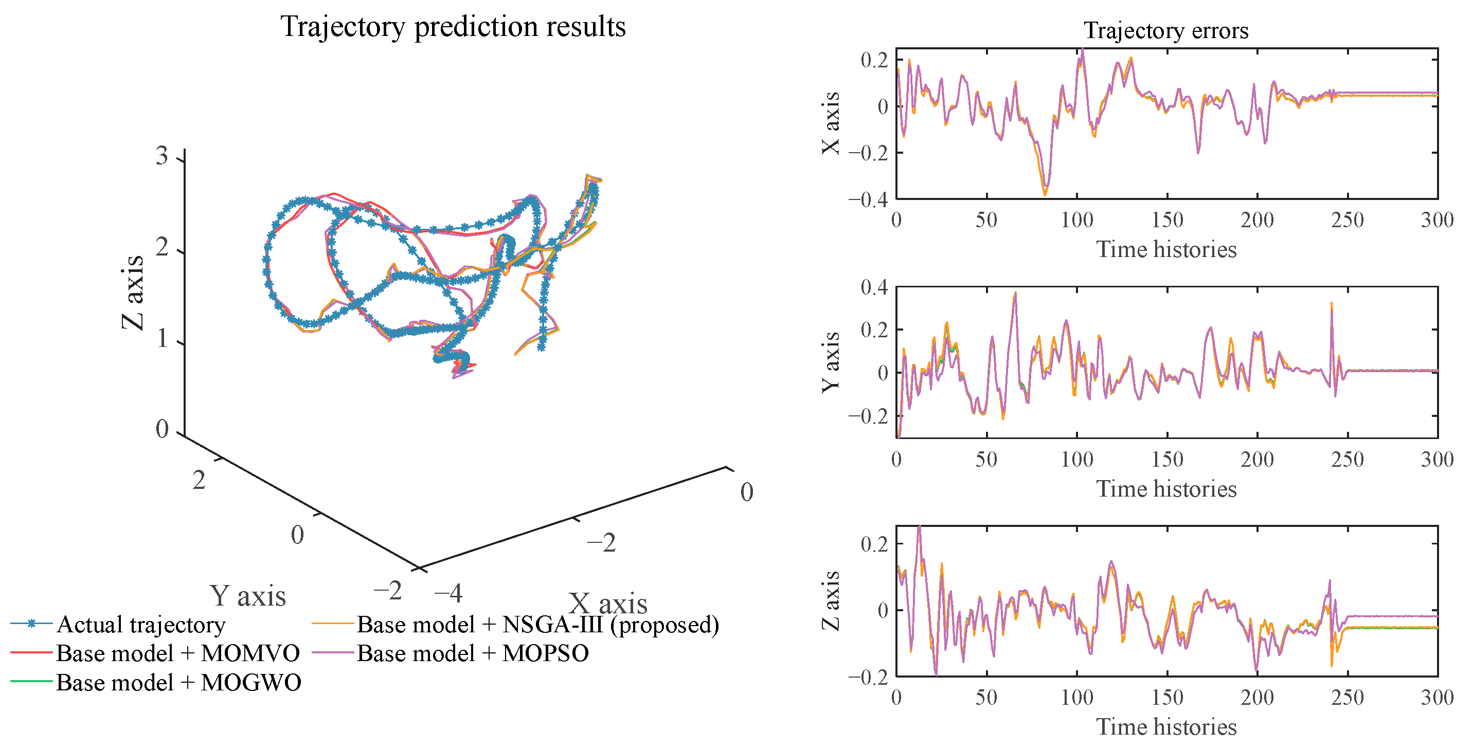
3.3. Comparison with Other Optimization Algorithms

To further validate the effectiveness of the proposed model, it is compared with three existing optimization algorithms, namely the multi-objective multi-verse optimization (MOMVO) [55], multi-objective grey wolf optimizer (MOGWO) [56], and multi-objective particle swarm optimization (MOPSO) [57]. They use the same models as base learners, but apply different multi-objective optimization algorithms to achieve ensemble learning. Thus, the prediction results can be obtained. The five-step ahead prediction results for dataset #1, dataset #2, dataset #3, and dataset #4 are shown in Figure 9, Figure 10, Figure 11 and Figure 12. Moreover, the corresponding evaluation metrics of different multi-objective ensemble models are shown in

Table 3. Evaluation metrics of different multi-objective ensemble models.

Dataset	Model	ADE	NLADE	FDE
#1	Base model + MOMVO	0.349	0.349	0.692
	Base model + MOGWO	0.349	0.349	0.693
	Base model + MOPSO	0.353	0.353	0.701
	Base model + NSGA-III (proposed)	0.346	0.346	0.685
#2	Base model + MOMVO	1.534	1.534	2.794
	Base model + MOGWO	1.663	1.663	2.953
	Base model + MOPSO	1.103	1.103	1.828
	Base model + NSGA-III (proposed)	0.783	0.783	1.425
#3	Base model + MOMVO	0.032	0.032	0.075
	Base model + MOGWO	0.032	0.032	0.074
	Base model + MOPSO	0.032	0.032	0.075
	Base model + NSGA-III (proposed)	0.029	0.029	0.068
#4	Base model + MOMVO	0.056	0.056	0.126
	Base model + MOGWO	0.056	0.056	0.126
	Base model + MOPSO	0.056	0.056	0.126
	Base model + NSGA-III (proposed)	0.051	0.051	0.118

. According to Figure 9, Figure 10, Figure 11 and Figure 12 and Table 3, the following can be observed:

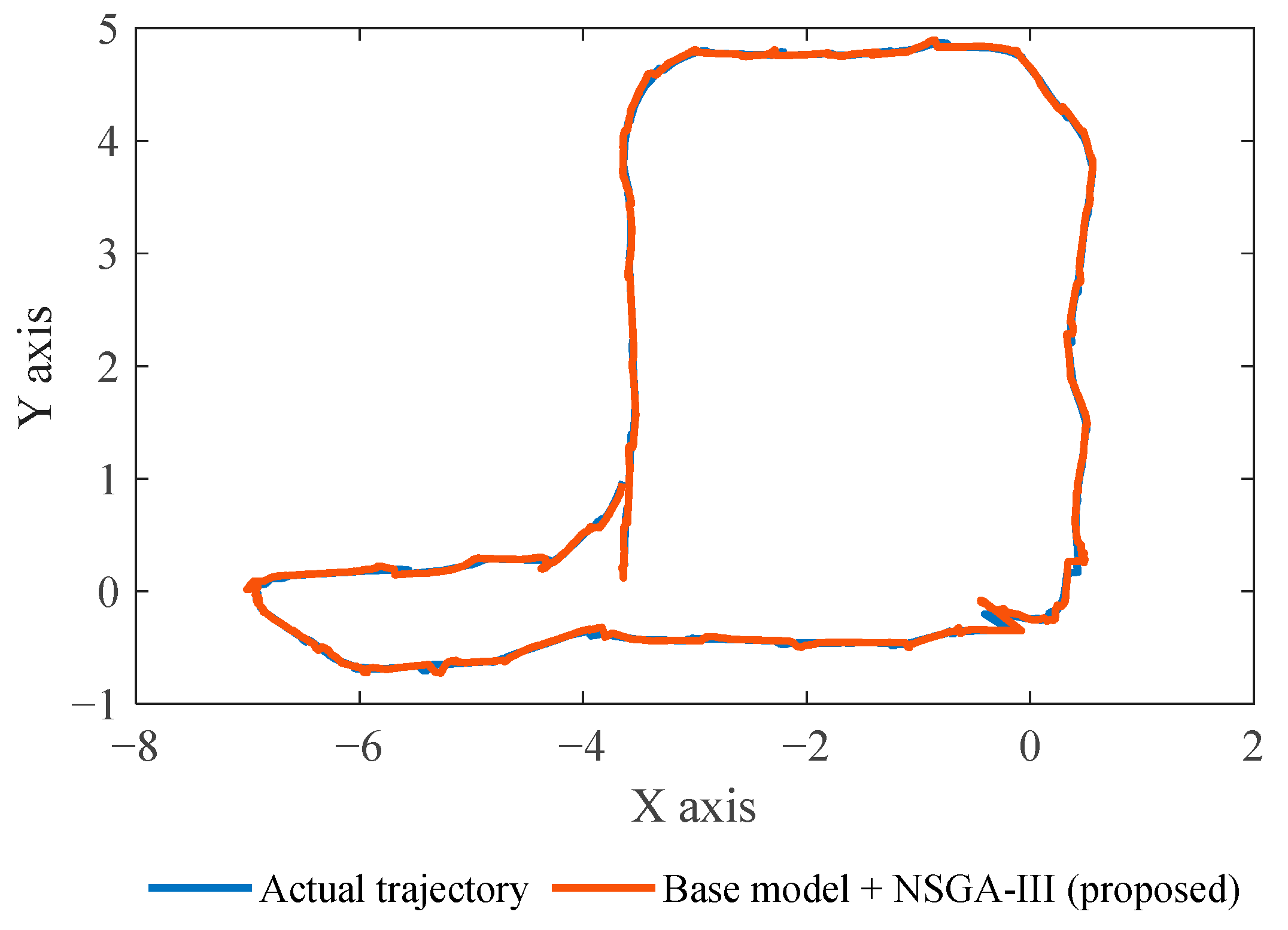
• All multi-objective optimization algorithms are effective for ensemble prediction of robot trajectory. Comparing the prediction error metrics based on the optimization algorithms with the five base learners, it can be found that the prediction error is further reduced. Moreover, the trajectory prediction results based on the optimization algorithms are all close to the actual trajectory of the robot movement, and satisfactory prediction accuracy has been achieved. This demonstrates that the comparative experimental settings of the multi-objective ensemble models are effective, and each algorithm is set reasonably, which helps to fairly evaluate the effectiveness of the proposed model.
• Compared with the other three optimization algorithms, the proposed model has the lowest prediction error. Taking dataset #2 as an example, the ADE, NLADE, and FDE of the MOMVO algorithm are 1.534, 1.534, and 2.794, respectively; the ADE, NLADE, and FDE of the MOGWO algorithm are 1.663, 1.663, and 2.953, respectively; and the ADE, NLADE, and FDE of the MOPSO algorithm are 1.103, 1.103, and 1.828, respectively. However, the ADE, NLADE, and FDE of the proposed MMP model are only 0.783, 0.783, and 1.425, respectively. This shows the superiority of the proposed model, which can achieve satisfactory prediction results on all datasets.
• By comparing the performance of each optimization algorithm on different datasets, it can be found that they have slight differences in the prediction results of datasets #1, #2, and #3. The reason for this phenomenon may be that the optimization goal is set to minimize the deviation and variance, which leads to relatively limited optimization space and a simple optimization problem. Different algorithms can approximate the global optimal solution, resulting in similar prediction results.

4. Additional Case for Inspection Robot

Inspection robots, which obey a prefix running trajectory and are sensitive to trajectory deviations, are important for periodicity detection under the IoT environment [58,59]. To verify the predictive performance of the proposed method on inspection tasks, a real robot trajectory series was used as in Figure 13. The trajectories were measured by odometer sensors on the Autolabor 2.5 robot platform. The whole time series contains 3848 data points, covering nearly three inspection routes. The first 2598 data points are utilized as the training set and the remaining 1250 data points are utilized as the testing set. To justify the case study, the testing set contains a complete inspection route.

The forecasting performance of the proposed model and benchmark models are shown in

Table 4. Evaluation metrics of ARMA, MLP, ENN, DESN, and LSTM models.

Model	ADE	NLADE	FDE
ARMA	0.034	0.035	0.055
MLP	0.028	0.028	0.035
ENN	0.023	0.023	0.033
DESN	0.022	0.022	0.031
LSTM	0.038	0.038	0.055
Base model + MOMVO	0.023	0.023	0.031
Base model + MOGWO	0.023	0.023	0.032
Base model + MOPSO	0.022	0.022	0.031
Base model + NSGA-III (proposed)	0.021	0.021	0.030

and Figure 14. It can be observed that the proposed model outperforms all the benchmark models, which indicates the effectiveness of the proposed model. According to the forecasting results of the proposed model in Figure 15, it can be observed that the proposed method can generate accurate forecasting results for a complete inspection trajectory, which indicates its effectiveness.

5. Generalization Analysis

In this study, the experiments separate the datasets into training and testing sets. The models are trained with only the training set, and the prediction results are generated with the testing set. In this manner, the data leak can be avoided. The prediction accuracy of the above experiments can reflect the generalization performance of the model.

Considering that a multi-learner multi-objective ensemble is very time-consuming, it is necessary to explore the update timeliness of the model to meet engineering needs. The experimental simulation used a Windows 10 desktop computer (Intel(R) Core(TM) i7-9700K CPU @ 3.60 GHz, 16 GB RAM). It can be seen from the modeling process that the ensemble weights generated by one experiment can effectively predict at least 300 points of data (10 Hz/20Hz). This shows that a set of ensemble weights can satisfy the prediction work of 15~30 s.

The computational time analysis of the multi-objective ensemble model with different optimization algorithms is shown in

Table 5. The computational time analysis of the proposed multi-objective ensemble model with different optimization algorithms.

Model	Dataset #1	Dataset #2	Dataset #3	Dataset #4
NSGA-III	138.71 s	143.53 s	189.22 s	177.99 s
MOMVO	141.11 s	146.78 s	188.15 s	180.31 s
MOGWO	145.62 s	151.25 s	193.43 s	184.94 s
MOPSO	139.77 s	145.83 s	190.66 s	182.81 s

; it can be seen that the modeling times of 2D datasets #1 and #2 are 138.71 s and 143.53 s, respectively, and the modeling times of 3D datasets #3 and #4 are 189.22 s and 177.99 s, respectively. Compared with other optimization algorithms, the computational time of NSGA-III is the shortest for datasets #1, 2, and 4, and it is the second shortest for dataset #3, proving the effectiveness of the proposed model.

To ensure the continuity of prediction tasks, the model can be embedded in parallel big data computing platforms such as MapReduce [60] and Apache Spark [61] to greatly reduce the processing time of data input–output and modeling analysis. Studies have shown that the collaboration of multiple work groups can reduce computing time by 20 to 45 times [62]. In this way, the modeling can be completed in just a few seconds, which effectively solves the problem of high-frequency iteration of the model. The continuously updated ensemble weights can also guarantee the generalization of the model.

6. Conclusions and Future Works

Robot trajectory prediction is an essential part of providing virtue trajectory information for the digital twin system. In the study, a novel MMP model was proposed for trajectory prediction. Five machine learning models including ARMA, MLP, ENN, DESN, and LSTM were adopted as base learners. Moreover, a high-level NSGA-III method was applied to automatically combine these base learners, generating an accurate and robust ensemble model. The proposed model was analyzed from different aspects. Its performance was also compared with three existing optimization algorithms. The results can be concluded as follows:

• The proposed multi-objective ensemble method is effective in improving the robot trajectory prediction accuracy of base learners. Its basic principle is to synchronously minimize the bias and variance of the model.
• The NSGA-III shows superiority in robot trajectory prediction. It significantly outperforms other optimization algorithms in dataset #1, and slightly outperforms other optimization algorithms in datasets #2 and #3.

The limitation of the proposed method is the generalization of the ensemble model to different data domains. In future works, we would like to perform research on improving the feasibility of the model to overcome the limitation. A more generalized model is expected from our future work, which could learn effective knowledge from uncoupled datasets and achieve accurate predictions on arbitrary datasets.

References

- Al-Okby, M.F.R.; Neubert, S.; Roddelkopf, T.; Thurow, K. Mobile Detection and alarming systems for hazardous gases and volatile chemicals in laboratories and industrial locations. Sensors 2021, 21, 8128. [Google Scholar] [CrossRef] [PubMed]
- Lee, C.-T.; Sung, W.-T. Controller Design of Tracking WMR system based on deep reinforcement learning. Electronics 2022, 11, 928. [Google Scholar] [CrossRef]
- Thamrongaphichartkul, K.; Worrasittichai, N.; Prayongrak, T.; Vongbunyong, S. A framework of IoT platform for autonomous mobile robot in hospital logistics applications. In Proceedings of the 2020 15th International Joint Symposium on Artificial Intelligence and Natural Language Processing (iSAI-NLP), Bangkok, Thailand, 18–20 November 2020; pp. 1–6. [Google Scholar]
- Patel, A.R.; Azadi, S.; Babaee, M.H.; Mollaei, N.; Patel, K.L.; Mehta, D.R. Significance of robotics in manufacturing, energy, goods and transport sector in internet of things (iot) paradigm. In Proceedings of the 2018 Fourth International Conference on Computing Communication Control and Automation (ICCUBEA), Pune, India, 16–18 August 2018; pp. 1–4. [Google Scholar]
- Zacharia, P.T.; Xidias, E.K. AGV routing and motion planning in a flexible manufacturing system using a fuzzy-based genetic algorithm. Int. J. Adv. Manuf. Technol. 2020, 109, 1801–1813. [Google Scholar] [CrossRef]
- Diez-Gonzalez, J.; Alvarez, R.; Prieto-Fernandez, N.; Perez, H. Local wireless sensor networks positioning reliability under sensor failure. Sensors 2020, 20, 1426. [Google Scholar] [CrossRef] [PubMed]
- Chang, L.; Shan, L.; Jiang, C.; Dai, Y. Reinforcement based mobile robot path planning with improved dynamic window approach in unknown environment. Auton. Robot. 2021, 45, 51–76. [Google Scholar] [CrossRef]
- Kousi, N.; Gkournelos, C.; Aivaliotis, S.; Lotsaris, K.; Bavelos, A.C.; Baris, P.; Michalos, G.; Makris, S. Digital twin for designing and reconfiguring human–robot collaborative assembly lines. Appl. Sci. 2021, 11, 4620. [Google Scholar] [CrossRef]
- Nabeeh, N.A.; Abdel-Basset, M.; Gamal, A.; Chang, V. Evaluation of production of digital twins based on blockchain technology. Electronics 2022, 11, 1268. [Google Scholar] [CrossRef]
- He, B.; Bai, K.-J. Digital twin-based sustainable intelligent manufacturing: A review. Adv. Manuf. 2021, 9, 1–21. [Google Scholar] [CrossRef]
- Havard, V.; Jeanne, B.; Lacomblez, M.; Baudry, D. Digital twin and virtual reality: A co-simulation environment for design and assessment of industrial workstations. Prod. Manuf. Res. 2019, 7, 472–489. [Google Scholar] [CrossRef]
- Pivarčiová, E.; Božek, P.; Turygin, Y.; Zajačko, I.; Shchenyatsky, A.; Václav, Š.; Císar, M.; Gemela, B. Analysis of control and correction options of mobile robot trajectory by an inertial navigation system. Int. J. Adv. Robot. Syst. 2018, 15, 172988141875516. [Google Scholar] [CrossRef]
- Duan, Z.; Liu, H.; Lv, X.; Ren, Z.; Junginger, S. Hybrid position forecasting method for mobile robot transportation in smart indoor environment. In Proceedings of the 2019 4th International Conference on Big Data and Computing, New York, NY, USA, 10 May 2019; pp. 333–338. [Google Scholar]
- Issa, H.; Tar, J.K. Preliminary design of a receding horizon controller supported by adaptive feedback. Electronics 2022, 11, 1243. [Google Scholar] [CrossRef]
- Murray, B.; Perera, L.P. A data-driven approach to vessel trajectory prediction for safe autonomous ship operations. In Proceedings of the 2018 Thirteenth International Conference on Digital Information Management (ICDIM), Berlin, Germany, 24–26 September 2018; pp. 240–247. [Google Scholar]
- QIiao, S.-J.; Han, N.; Zhu, X.-W.; Shu, H.-P.; Zheng, J.-L.; Yuan, C.-A. A dynamic trajectory prediction algorithm based on Kalman filter. Acta Electonica Sin. 2018, 46, 418. [Google Scholar]
- Xing, Y.; Wang, G.; Zhu, Y. Application of an autoregressive moving average approach in flight trajectory simulation. In Proceedings of the AIAA Atmospheric Flight Mechanics Conference, Washington, DC, USA, 13–17 June 2016; p. 3846. [Google Scholar]
- Heravi, E.J.; Khanmohammadi, S. Long term trajectory prediction of moving objects using gaussian process. In Proceedings of the 2011 First International Conference on Robot, Vision and Signal Processing, Kaohsiung, Taiwan, 21–23 November 2011; pp. 228–232. [Google Scholar]
- Liu, H.; Yang, R.; Duan, Z.; Wu, H. A hybrid neural network model for marine dissolved oxygen concentrations time-series forecasting based on multi-factor analysis and a multi-model ensemble. Engineering 2021, 7, 1751–1765. [Google Scholar] [CrossRef]
- Yang, R.; Liu, H.; Nikitas, N.; Duan, Z.; Li, Y.; Li, Y. Short-term wind speed forecasting using deep reinforcement learning with improved multiple error correction approach. Energy 2022, 239, 122128. [Google Scholar] [CrossRef]
- Seker, M.Y.; Tekden, A.E.; Ugur, E. Deep effect trajectory prediction in robot manipulation. Robot. Auton. Syst. 2019, 119, 173–184. [Google Scholar] [CrossRef]
- Sun, L.; Yan, Z.; Mellado, S.M.; Hanheide, M.; Duckett, T. 3DOF pedestrian trajectory prediction learned from long-term autonomous mobile robot deployment data. In Proceedings of the 2018 IEEE International Conference on Robotics and Automation (ICRA), Brisbane, QLD, Australia, 21–25 May 2018; pp. 5942–5948. [Google Scholar]
- Zhang, J.; Liu, H.; Chang, Q.; Wang, L.; Gao, R.X. Recurrent neural network for motion trajectory prediction in human-robot collaborative assembly. CIRP Ann. 2020, 69, 9–12. [Google Scholar] [CrossRef]
- Nikhil, N.; Tran Morris, B. Convolutional neural network for trajectory prediction. In Proceedings of the European Conference on Computer Vision (ECCV) Workshops, Munich, Germany, 8–14 September 2018; pp. 1–11. [Google Scholar]
- Chen, C.; Liu, H. Medium-term wind power forecasting based on multi-resolution multi-learner ensemble and adaptive model selection. Energy Convers. Manag. 2020, 206, 112492. [Google Scholar] [CrossRef]
- Liu, H.; Yang, R.; Wang, T.; Zhang, L. A hybrid neural network model for short-term wind speed forecasting based on decomposition, multi-learner ensemble, and adaptive multiple error corrections. Renew. Energy 2021, 165, 573–594. [Google Scholar] [CrossRef]
- Kim, Y.; Hur, J. An ensemble forecasting model of wind power outputs based on improved statistical approaches. Energies 2020, 13, 1071. [Google Scholar] [CrossRef]
- Liu, H.; Duan, Z.; Chen, C. A hybrid multi-resolution multi-objective ensemble model and its application for forecasting of daily PM2.5 concentrations. Inf. Sci. 2020, 516, 266–292. [Google Scholar] [CrossRef]
- Ribeiro, M.H.D.M.; dos Santos Coelho, L. Ensemble approach based on bagging, boosting and stacking for short-term prediction in agribusiness time series. Appl. Soft Comput. 2020, 86, 105837. [Google Scholar] [CrossRef]
- Wang, F.; Li, Y.; Liao, F.; Yan, H. An ensemble learning based prediction strategy for dynamic multi-objective optimization. Appl. Soft Comput. 2020, 96, 106592. [Google Scholar] [CrossRef]
- Wang, H.; Yang, Z.; Shi, Y. Next location prediction based on an adaboost-markov model of mobile users. Sensors 2019, 19, 1475. [Google Scholar] [CrossRef] [PubMed]
- Rasouli, A.; Kotseruba, I.; Tsotsos, J.K. Pedestrian action anticipation using contextual feature fusion in stacked rnns. arXiv 2020, arXiv:2005.06582. [Google Scholar]
- Xu, Y.; Liu, H. Spatial ensemble prediction of hourly PM2. 5 concentrations around Beijing railway station in China. Air Qual. Atmos. Health 2020, 13, 563–573. [Google Scholar] [CrossRef]
- Weisberg, M. Robustness analysis. Philos. Sci. 2006, 73, 730–742. [Google Scholar] [CrossRef]
- Liu, Y.; Gong, C.; Yang, L.; Chen, Y. DSTP-RNN: A dual-stage two-phase attention-based recurrent neural network for long-term and multivariate time series prediction. Expert Syst. Appl. 2020, 143, 113082. [Google Scholar] [CrossRef]
- Lin, C.-Y.; Hsieh, Y.-M.; Cheng, F.-T.; Huang, H.-C.; Adnan, M. Time series prediction algorithm for intelligent predictive maintenance. IEEE Robot. Autom. Lett. 2019, 4, 2807–2814. [Google Scholar] [CrossRef]
- Chen, W.; Xu, H.; Chen, Z.; Jiang, M. A novel method for time series prediction based on error decomposition and nonlinear combination of forecasters. Neurocomputing 2021, 426, 85–103. [Google Scholar] [CrossRef]
- Zhang, Y.; Wang, X.; Tang, H. An improved Elman neural network with piecewise weighted gradient for time series prediction. Neurocomputing 2019, 359, 199–208. [Google Scholar] [CrossRef]
- Wang, Z.; Yao, X.; Huang, Z.; Liu, L. Deep echo state network with multiple adaptive reservoirs for time series prediction. IEEE Trans. Cogn. Dev. Syst. 2021, 13, 693–704. [Google Scholar] [CrossRef]
- Yan, B.; Aasma, M. A novel deep learning framework: Prediction and analysis of financial time series using CEEMD and LSTM. Expert Syst. Appl. 2020, 159, 113609. [Google Scholar]
- Zhou, Z. Ensemble Methods: Foundations and Algorithms; Taylor & Francis—Chapman and Hall/CRC: New York, NY, USA, 2012. [Google Scholar]
- Deb, K.; Jain, H. An evolutionary many-objective optimization algorithm using reference-point-based nondominated sorting approach, part I: Solving problems with box constraints. IEEE Trans. Evol. Comput. 2013, 18, 577–601. [Google Scholar] [CrossRef]
- Das, I.; Dennis, J.E. Normal-boundary intersection: A new method for generating the Pareto surface in nonlinear multicriteria optimization problems. SIAM J. Optim. 1998, 8, 631–657. [Google Scholar] [CrossRef]
- Taieb, S.B.; Atiya, A.F. A bias and variance analysis for multistep-ahead time series forecasting. IEEE Trans. Neural Netw. Learn. Syst. 2016, 27, 62–76. [Google Scholar] [CrossRef]
- Wang, C.; Zhang, S.; Xiao, L.; Fu, T. Wind speed forecasting based on multi-objective grey wolf optimisation algorithm, weighted information criterion, and wind energy conversion system: A case study in Eastern China. Energy Convers. Manag. 2021, 243, 114402. [Google Scholar] [CrossRef]
- Liu, H.; Yang, R. A spatial multi-resolution multi-objective data-driven ensemble model for multi-step air quality index forecasting based on real-time decomposition. Comput. Ind. 2021, 125, 103387. [Google Scholar] [CrossRef]
- Wang, J.; Wang, R.; Li, Z. A combined forecasting system based on multi-objective optimization and feature extraction strategy for hourly PM2.5 concentration. Appl. Soft Comput. 2022, 114, 108034. [Google Scholar] [CrossRef]
- Felfel, H.; Ayadi, O.; Masmoudi, F. Pareto optimal solution selection for a multi-site supply chain planning problem using the VIKOR and TOPSIS methods. Int. J. Serv. Sci. Manag. Eng. Technol. 2017, 8, 21–39. [Google Scholar] [CrossRef][Green Version]
- Taleizadeh, A.A.; Niaki, S.T.A.; Aryanezhad, M.-B. A hybrid method of Pareto, TOPSIS and genetic algorithm to optimize multi-product multi-constraint inventory control systems with random fuzzy replenishments. Math. Comput. Model. 2009, 49, 1044–1057. [Google Scholar] [CrossRef]
- WANG, D.; LI, S. Lightweight optimization design of side collision safety parts for BIW based on pareto mining. China Mech. Eng. 2021, 32, 1584. [Google Scholar]
- Saeedi, S.; Carvalho, E.D.C.; Li, W.; Tzoumanikas, D.; Leutenegger, S.; Kelly, P.H.J.; Davison, A.J. Characterizing visual localization and mapping datasets. In Proceedings of the 2019 International Conference on Robotics and Automation (ICRA), Montreal, QC, Canada, 20–24 May 2019; pp. 6699–6705. [Google Scholar]
- Zhang, G.; Ouyang, R.; Lu, B.; Hocken, R.; Veale, R.; Donmez, A. A displacement method for machine geometry calibration. CIRP Ann. 1988, 37, 515–518. [Google Scholar] [CrossRef]
- Huang, C.-H. A non-linear inverse vibration problem of estimating the external forces for a system with displacement-dependent parameters. J. Sound Vib. 2001, 248, 789–807. [Google Scholar] [CrossRef]
- Keil, C.; Craig, G.C. A displacement-based error measure applied in a regional ensemble forecasting system. Mon. Weather. Rev. 2007, 135, 3248–3259. [Google Scholar] [CrossRef]
- Mirjalili, S.; Jangir, P.; Mirjalili, S.Z.; Saremi, S.; Trivedi, I.N. Optimization of problems with multiple objectives using the multi-verse optimization algorithm. Knowl. Based Syst. 2017, 134, 50–71. [Google Scholar] [CrossRef]
- Mirjalili, S.; Saremi, S.; Mirjalili, S.M.; Coelho, L.d.S. Multi-objective grey wolf optimizer: A novel algorithm for multi-criterion optimization. Expert Syst. Appl. 2016, 47, 106–119. [Google Scholar] [CrossRef]
- Mostaghim, S.; Teich, J. Strategies for finding good local guides in multi-objective particle swarm optimization (MOPSO). In Proceedings of the 2003 IEEE Swarm Intelligence Symposium. SIS’03 (Cat. No.03EX706), Indianapolis, IN, USA, 26–26 April 2003; pp. 26–33. [Google Scholar]
- Tao, T. Research on intelligent robot patrol route based on cloud computing. In Proceedings of the 2019 International Conference on Computer Network, Electronic and Automation (ICCNEA), Xi’an, China, 27–29 September 2019; pp. 511–516. [Google Scholar]
- Liu, H. Robot Systems for Rail Transit Applications; Elsevier: Amsterdam, Netherlands, 2020. [Google Scholar]
- Bendre, M.; Manthalkar, R. Time series decomposition and predictive analytics using MapReduce framework. Expert Syst. Appl. 2019, 116, 108–120. [Google Scholar] [CrossRef]
- Zaharia, M.; Xin, R.S.; Wendell, P.; Das, T.; Armbrust, M.; Dave, A.; Meng, X.; Rosen, J.; Venkataraman, S.; Franklin, M.J. Apache spark: A unified engine for big data processing. Commun. ACM 2016, 59, 56–65. [Google Scholar] [CrossRef]
- Meng, X.; Bradley, J.; Yavuz, B.; Sparks, E.; Venkataraman, S.; Liu, D.; Freeman, J.; Tsai, D.; Amde, M.; Owen, S. Mllib: Machine learning in apache spark. J. Mach. Learn. Res. 2016, 17, 1235–1241. [Google Scholar]